1. Introduction
The dense GNSS (Global Navigation Satellite System) networks provide detailed information to explore the crustal deformation, such as the secular tectonic movements, the co- and postseismic displacements, the loading effects caused by mass redistributions, the thermal expansion, and other unknown geophysical processes [
1,
2,
3,
4,
5]. Improved spatio-temporal resolution of the deformation solutions makes it possible to detect weak and transient crustal signals, which were hidden in the noise of previous solutions [
6,
7,
8,
9,
10,
11,
12]. The transient deformation origin should be nontectonic as well as tectonic, including the processes occurring at active fault zones, volcanic process, and so on. In particular, understanding the tectonic transient characterizations and spatial-temporal variations is crucial for exploring the seismic hazards. To capture these short-term irregular events, however, the biggest challenge is the separation of the geophysical signals from the noise and unknown system errors.
Previous research revealed that there existed a spatially correlated error (called as Common Model Error, CME) in the GNSS solutions [
7,
12]. Although the origin of the CME is not thoroughly understood yet, it can be isolated given that spatial correlation range of the CME is regional (it reaches up to 2000 km) [
11], while the spatial coherent range of the transient event is only local (it covers less than 100 km) [
7,
9,
10,
11]. Wdowinski et al. [
7] employed stacking filtering to remove the CME and improved the displacement resolutions for the 1992 Lander earthquake. Liu et al. [
9] estimated the CME in a much larger region to ensure the CME estimation was not contaminated by local nonsecular deformation. Finally, after the removal of CME, the original time series reduced the scatter while maintaining deformation signals of volcanic activities. Tian et al. [
11] applied the correlation-weighted spatial filtering algorithm to extract coherent signals from a dense GPS network and detected subtle tectonic deformation signals. Thus, the regional GNSS network analyses provide ideal means to detect and isolate the CME and then to enhance the signal-to-noise ratio of the solution series. Several approaches, such as stacking, principal component analysis (PCA), independent component analysis (ICA), etc., have been proposed in GNSS position time series analysis to estimate the CME [
7,
8,
9,
10,
11,
12,
13,
14,
15,
16,
17].
However, the nature and the wavelength of CME are still unclear considering its temporal-spatial diversity and multi-inducements. The proper characterization and modeling of sites’ coordinate time series are critical in improving the coordinate accuracy from regional network measurements. Especially for the places characterized by complex tectonic and nontectonic movements, such as the Chuandian region of China (
Figure 1). The region is in the east of the Tibetan Plateau and is the front edge of NE compression induced by the Indian plate where the activities of strong earthquakes are intense. In addition, abundant precipitation and hydrologic cycle also induce obvious crustal deformation in the region. Various filtering techniques have been developed to detect and isolate the CME in Chuandian region. Li et al. [
18] applied the Improved Principle Component Analysis on Yunnan Province and reduced the average error of the position time series. Pan et al. [
5] had discussed the period of 3–4 years signals in CME of Eastern Tibetan Plateau which were highly related to hydrologic loading displacements. Liu et al. [
13] applied the ICA to analyze continuous GPS data in Chuandian region and discussed the mechanism of the CME with 40 sites. They explained that the seasonal variations in CME were mainly due to loading effects of the surface atmosphere and soil moisture loadings. Similar discussions were also shown in Sheng et al. [
19] and Yuan et al. [
20]. In addition, Yuan et al. [
20] also expressed that the CME in Hongkong was highly related to the high-order ionospheric effects.
In this paper, we focus on common mode component (CMC) of site displacements caused by mass loadings and try to explore the CME origin in Chuandian region. We firstly apply the PCA to daily stations coordinate time series to extract the original CME in the region. And we also estimate the CMC of the site displacements caused by atmospheric and soil moisture mass loadings. In addition, we evaluate the corrected CME in the GPS residual time series which have subtracted the calculated daily site displacements caused by atmospheric and soil moisture mass loadings. Finally, we demonstrate the contributions of the two mass loadings to the CME in Chuandian region.
2. Data Source and CME Processing Methods
Crustal Movement Observation Network of China (CMONOC) was implemented since 1999 and had 260 continuous stations until 2011. CMONOC consists not just of 260 GNSS continuous observations, but also of supplements with Very Long Baseline Radio Interferometry (VLBI), Satellite Ranging (SLR), precise leveling, and gravity observation in a few sites. It provides abundant continuous GPS observations for crustal deformation monitoring with relatively high spatial resolution (dozens of kilometers) and long time scale (more than 8 years). In this study, GPS measurements during 2011 to 2017 obtained from 51 sites in the Chuandian region (
Figure 1 and
Table 1) are used to derive the position time series with integrated Geodetic Platform Of Shanghai Astronomical Observatory (iGPOS,
http://www.shao.ac.cn/shao_gnss_ac) [
21]. The processing models and strategies for the daily solution details are available in Chen et al. [
21] and references therein.
2.1. Acquisition of GPS Residual Coordinate Time Series
We applied QOCA software to obtain the GPS residual coordinate time series of vertical component [
2]. The daily coordinate solutions with larger formal uncertainties (>1000 mm) were removed. The non-geophysical offsets and coseismic displacements were also removed from the time series. As we know, the CME was found when comparing the coordinate residual time series which had deducted all known geophysical information. The secular rates and the seasonal variations usually indicate the plate motions and mass redistributions separately. Thus, we estimated parameters of model that includes offsets, linear trends, and seasonal (annual and semiannual) terms and removed these modeled terms to obtain the resulting position time series called as
residual time series in this paper [
2,
17]. Besides, we also removed the residuals that exceeded the thresholds of 40 mm [
15,
17]. Then, we analyzed the residual time series to explore the potential signals in CME.
2.2. Principle Component Analysis (PCA)
The PCA decomposes the time series into various spatial and temporal coherent orthogonal modes. It does not require a preset orthogonal basis function but constructs an orthogonal feature vector by orthogonally decomposing a set of related data itself. With these orthogonal feature vectors as the basis, the corresponding coefficients constitute the principal components. The principal components are arranged in descending order of the eigenvalues, and the first few principal components can cover most of the energy in the original data set. Therefore, an important application of PCA is to find a small number of principal components to represent the basic characteristics of the original data set, which plays a role in dimensionality reduction and denoising [
12,
14,
15,
18].
For a regional GNSS network of
n stations, the daily station residual time series spanning
m days can be written as
X(ti,xj) (
i = 1,2,3…,m;
j = 1,2,3…n). Firstly, we construct the covariance matrices
B, the i-th row
j-th column element in the covariance matrix
B can be expressed as [
12]
The symmetric matric
B can be decomposed given by
B =
V·Λ·VT, where Λ is a matrix with
k non-zero diagonal eigenvalues and eigenvector matrix
VT is an (n × n) matrix. In most cases with geodetic data, the rank of matrix
B is usually full. From linear algebra, we can expand any matrix of rank n by n orthonormal vector basis. Thus, the data matrix X(
ti,
xj) can be expressed by the orthonormal function basis
v:
The ak(ti) is the so-called kth principal component (PC) for matrix X, and it represents a temporal signature of the mode. The vk(xj) is ak(ti) corresponding eigenvector, which represents the spatial distribution of the mode. The principal component ak(ti) and the eigenvectors vk(xj) together are considered as mode k. We arrange the eigenvectors with descending eigenvalues to identify the first few PCs to represent the biggest contributors to the variance of the network residual time series.
3. Results: CME Patterns in Chuandian Region
We extracted the residual time series by removing the known periodic variations and linear trends. Then, we applied the PCA on GPS residual time series to derive regional CME and investigated its spatial distribution.
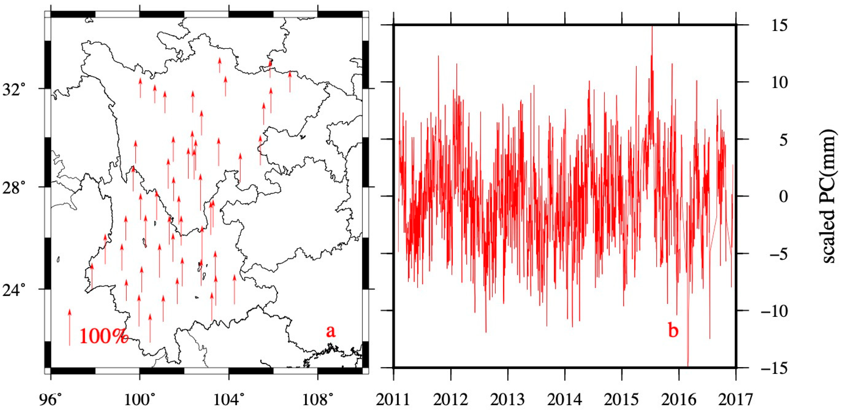
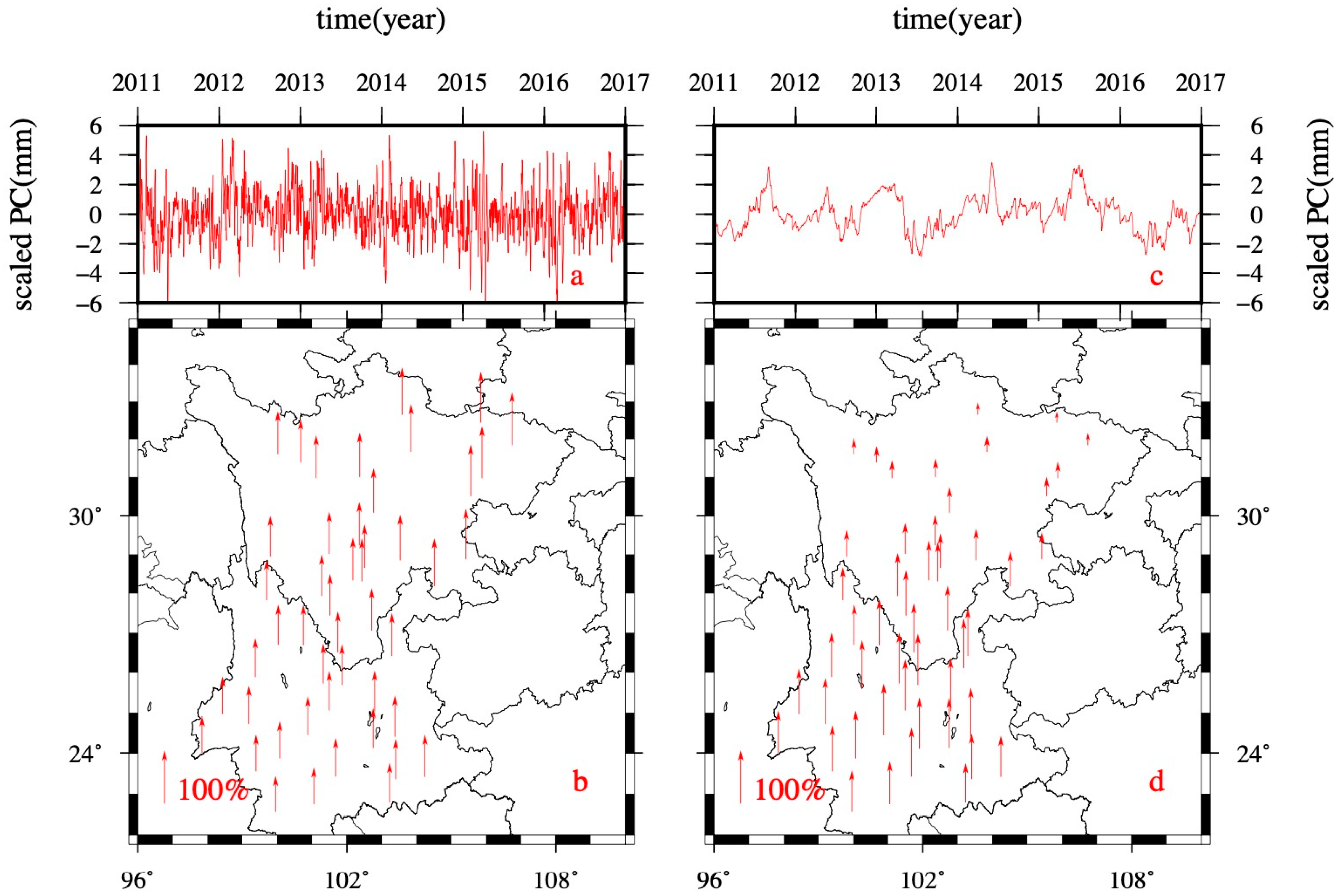
Figure 2 shows the spatial and temporal patterns of the first PC derived from PCA. The PCA obtained nearly uniformly distributed normalized spatial eigenvectors for the first PC time series, with average normalized amplitudes (absolute values) of 73.9%. The minimum normalized amplitude is 52.5%. We use the criterion from Dong et al. [
12] to define the CME as the mode for which most sites (more than 50%) have significant normalized responses (larger than 25%), and the eigenvalues of this mode exceed 1% of the summation of all eigenvalues. Thus, we treat the first PC from PCA as the CME in Chuandian region. However, we cannot directly classify the CME as signal or noise.
As we know, the network residual time series contain multi modes from network common (in the region reach up to 2000 km [
2,
11]) to local common (the spatial coherent range of the transient event covers less than 100 km [
9,
11]) and site-dependent, such as the CME, various local effects, and random noises. The PCA approach assumes spatiotemporal PCs are orthogonal to each other. However, the PCA-derived CME series are not totally uncorrelated with the local effects or random noises. It is hard for PCA to decompose the similar contributions components in actual network residual time series. The PCA-decomposed principal components and their corresponding eigenvectors are arranged by the eigenvalue through descending order. Thus, each principal component is a mixture of several mechanisms. We are unable to identify the potential geophysical mechanisms or study the subtle signals in GPS observations. For example, the annual items in the GNSS station coordinate series come mainly from the contributions of mass variations including atmosphere pressure, ocean loading, snow, and soil moisture variations. When we use PCA for the annual analysis, the contributions of these mechanisms cannot be separated [
17]. The PCA algorithm cannot separate the contributions of these mechanisms in the original sequence. Then, we would also conclude the CME in Chuandian region is the mixture of some unknown geophysical signals and random noises.
Thus, the CME is usually composed of two parts: (1) the observation and model errors and (2) the potential geophysical signals. (1) The observation and model errors. The observation errors are mainly induced by observation instrument errors or inaccurate analysis methods. The model errors are mainly ascribed to the multipath model and the incomplete satellite light pressure model. Besides, the mode errors of the atmospheric delay, ionospheric delay, and systematic reference frame errors are also the potential causes. (2) The potential geophysical signals. The widely used GPS coordinate time series analysis mainly estimates the initial position, velocity, and annual and subannual terms of the stations. Some studies have demonstrated that the plate motions and subsurface mass redistributions’ seasonal variations are the main contributors to the linear and seasonal variations separately [
1,
2,
3]. The seasonal terms are usually modeled as sinusoids [
2]. However, the sinusoid models only represent the annual and subannual signals in GPS time series, and they are too simplified to estimate the truth geophysical processes of mass loading variations accurately, especially in the daily timescales. All the unmodeled deformation signals are left in the residual time series [
12,
14]. Then, when we apply the PCA method, the effects of the unmodeled geophysical process will be absorbed into the uniformly distributed modes and the randomly distributed modes. Thus, the first PC derived from PCA, as well as the CME, may contain the mismodeled signals of the mass redistributions. Besides, the high-order modes extracted from PCA are usually related to a few stations and presumably reflect local effects. The mechanism of the high-order-mode PCs is an open question we leave for future study.
Since there is a clue that signal sources to the CME may relate the mass redistributions, we make deep explorations of the mass loadings. We check the common mode components (CMCs) of the mass loading variations which have removed the linear trend and annual and subannual variations.
4. Subtracting the Daily Site Displacements of Known Geophysical Sources
For the Chuandian region, only the first PC of the vertical components satisfy our criteria for CME; we also call these original CME in this paper. The CME of the regional network may contain contributions from some unknown geophysical sources. To explore the nature of the CME, an approach is to subtract the contributions of sources from the GPS observations to obtain the corrected CME, then study the relation between original CME with corrected CME. It is well known that mass loading variations can cause seasonal variations in regional GPS positions time series, especially in the vertical direction. We also usually use the sinusoids model to describe the seasonal variations of mass loadings. However, we also notice that the mass loadings vary daily and may induce obvious displacements. In this section, we examine the distributions and magnitudes of the daily variations of the mass loadings. We obtain CMCs of two geophysical processes which would potentially make a part of contributions to the CME in the region.
4.1. Daily Atmospheric Mass Loading
The 6 hour sampling National Center for Environmental Prediction (NCEP) reanalysis surface atmosphere pressure data [
22] from 2011 to 2017 are used to calculate the displacements at each site in the study. We calculate the daily site displacements from the atmosphere pressure variations by Farrell [
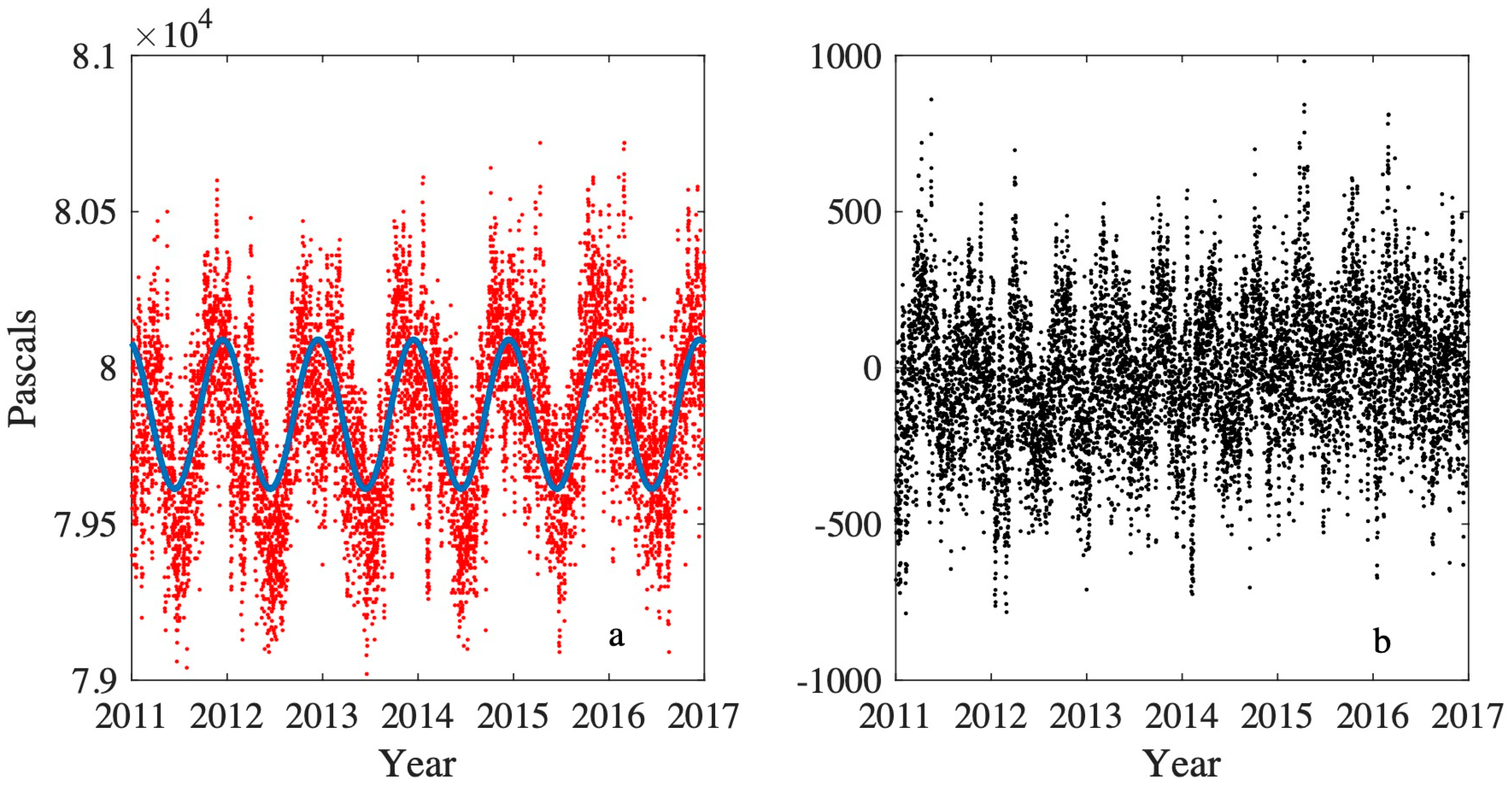
23] elastic Green’s function approach. To verify daily variations of atmospheric pressure, we first check the atmosphere pressure data at some grids located in Chuandian region (
Figure 3,
Figures S1–S3). After removing the seasonal and linear variations of atmosphere pressure, we still see obvious residual variations of the atmosphere pressure. The daily atmosphere pressure residual varies dramatically especially in the beginning of each year.
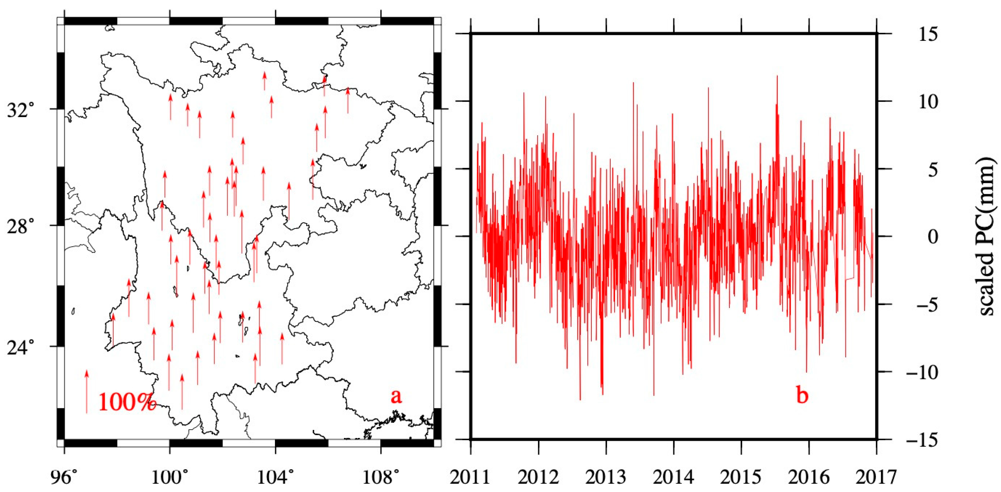
We also subtracted the trends and seasonal terms of calculated daily site displacements caused by atmospheric loading. The left residual time series would especially highlight the daily displacement variations for the atmosphere mass loading (ATML). Then, we performed the PCA method to identify the principal components in the site displacements inducted by ATML in Chuandian region. The first PC is somehow spatially uniform in the whole region, and its average spatial response is about 77.9%. The results are shown in
Figure 4a. The second and high-order PC temporal variations are too small (less than 1mm); thus, we mainly treat the first components as the common mode component (CMC) in ATML.
4.2. Daily Soil Moisture Mass Loading
The hydrological loadings are also important contributors to the seasonal variations in Chuandian region [
24]. We applied the NCEP reanalysisⅡ (
https://www.esrl.noaa.gov/psd/data/gridded/data.ncep.reanalysis2.gaussian.html) daily sampling soil moisture data to calculate site displacements by Farrell [
23] elastic Green’s function approach. We removed the seasonal variations and linear trends of daily site displacements series caused by soil moisture mass loading (SML). Then, we also performed the PCA to get the principal components in the SML time series. The first PC of the daily SML in Chuandian region are shown in
Figure 4b. We also obtain giant variations of the soil moisture loading residuals in the region. The average spatial response for the soil moisture loading first PC is 70.4%. In the northern Chuandian region, the spatial response is about 20%-40%. And the spatial responses are mostly more than 70% in the southern region. According to the CME criterion from Dong et al. [
12], we treat the first PC of the soil moisture loading as the CMC.
Dong et al. [
2] have demonstrated that the site’s vertical seasonal variations are mostly affected by mass redistributions. After the removal of the seasonal terms of the GPS quasi-observations, the seasonal terms of the mass-loading-caused displacements are subtracted from the quasi-observation series. However, the mass-redistribution-caused daily-variation site displacements and inter-annual-site displacements will remain in the residual series. Thus, we would consider the daily variations of atmosphere pressure and soil moisture loading to be connected to the CME. Besides, we also calculated the CMCs for snow and nontidal-ocean-loadings-induced deformation in Chuandian region, but both of the two CMCs are less than 0.1 mm. Thus, we excluded the relationship between CME and snow/nontidal ocean mass loadings, and we will not have deep discussion of their effects in this study.
4.3. Corrected CME of GPS Residuals after Subtracting the Known Geophysical Sources
We firstly subtracted the daily atmosphere and soil mass loadings that caused site displacements from the GPS station position residual observations and then applied the PCA to obtain the mass loadings corrected CME.
Figure 5 shows corrected CME, which reduces the RMS (Root Mean Squares) of the CME from 4.19 to 3.56 mm. To quantitatively evaluate the contributions of the atmospheric and soil moisture loadings to the CME, we defined a measure termed the
RMS Reduction Ratio, expressed as follows:
RMSoriginal_CME is the RMS of the original CME time series, RMScorrected_CME is the RMS of corrected CME series after the daily atmosphere and soil loadings are corrected. The RMS Reduction Ratio reflects the corrected loading effects in the CME. The ratio with a value of 0 would indicate that the mass loadings have no contributions to the CME. The ratio with a value of 1.0 would indicate that the CME only contains the ATML and SML signals. The calculated RatioRMS_reduction is about 15%, which reflects that the ATML and SML CMCs can contribute almost 15% to the CME in Chuandian region.
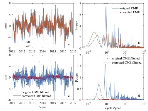
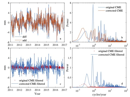
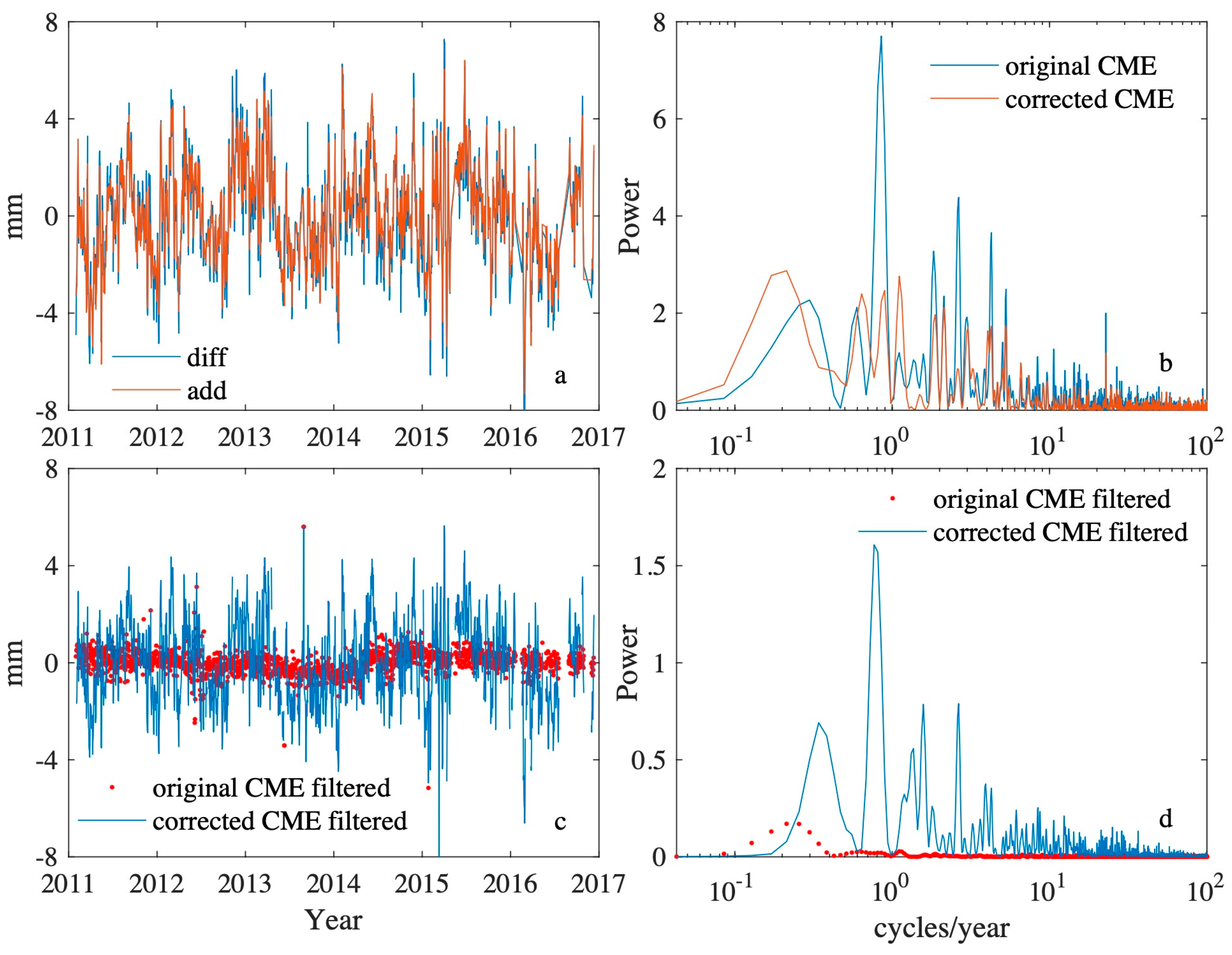
Thus, the original CME contains the daily variations of mass loadings while the corrected CME has excluded such loading effects. To present the difference between original CME and corrected CME, we subtracted the corrected CME in the original CME and get the “diff” series shown in
Figure 6a. The “diff” series is actually the mismodeled daily mass loading variations. It is the geophysical signal part to CME, which comes from the GPS time series analysis methods. Meanwhile, we sum the CMCs of ATML and SML as “add” shown in
Figure 6a. The two series “diff” and “add” actually represent the difference of two CME and daily variations of two geophysical processes, respectively. The two series, “diff” and “add” are highly consistent with a correlation coefficient 0.95, which implies that the mismodeled CMCs of ATML and SML fully leak into the uniformly distributed CME in Chuandian region.
Figure 6b represents the power spectral densities of original CME and corrected CME in the region. We notice that the power of the corrected CME has reduced in a wide range of frequencies, which shows that the temporal characteristics of CME are still unknown.
Figure 6a,b show comparisons of the original CME and corrected CME time series.
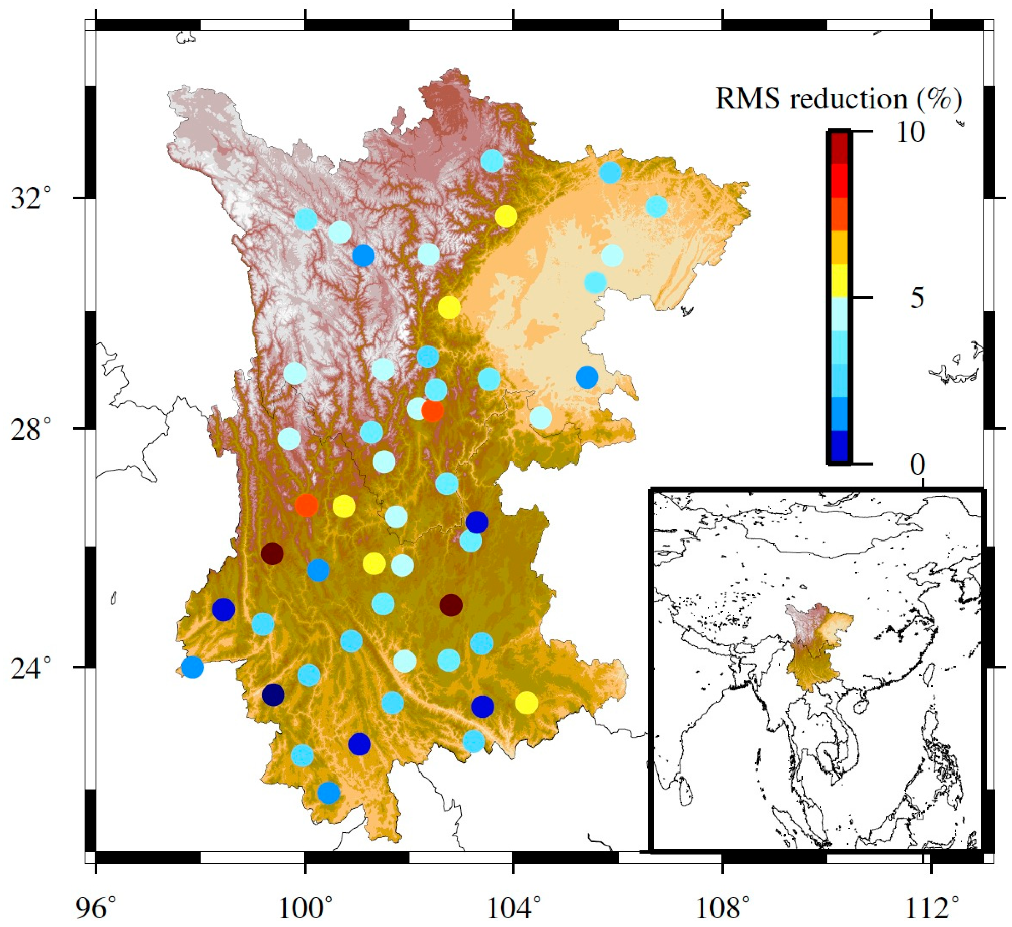
Besides, we remove the original CME and corrected CME separately from the GPS height time series and calculate the RMS reduction of the filtered GPS time series after the removal of the two CME. The reduction
RMSredtn = (RMScorrected_CME - RMSoriginal_CME)/RMSGPS represents the relative magnitude of the CME in observed time series, and it is a common statistic to assess the impact of daily loading effects in CME. The reductions reduce at 50 stations (
Figure 1), and the RMS
redtn is reduced by an average of 4.1%. The GPS RMS
redtn reductions directly represent the differences between the two CME in GPS observations. The average RMS
redtn 4.1% is actually the mismodeling daily mass loadings effects in GPS. For most of the stations located in Chuandian region, we are able to explain a part of CME by the modeling daily atmosphere and soil moisture mass changes.
It is interesting to compare the average daily scatter of the original CME filtered time series and corrected CME filtered time series (
Figure 6c). The average daily scatter in
Figure 6c is calculated using the sum of the residual values divided by station number. Significant difference is represented in the filtered two daily scatter time series. The results imply the existence of mass loading CMCs in the CME in Chuandian region (
Figure 6c,d). The frequency analysis shows that the left daily mass loadings explained most of the scatter, but there is still a low-frequency signal. As the data span is only 6 years in this study, it is hard to make a detailed discussion about the low-frequency signals. Then we leave this as an open question. Thus, daily variations of mass loadings explain a part of the CME in the region.
5. Conclusions
In this study, we estimated the CME in Chuandian region by PCA and explored the possible origin in the CME time series by examining the time series of 51 CMONOC stations over a 6 year period. The PCA is a useful approach to identify the principle components in the spatial distributions of the CME [
5,
9,
12,
15]. The spatial distributions of CME are close to uniform in the region.
The CME identified by PCA may contain potential geophysical process signals. Based on the theory that the CME is composed of two parts: the error one and the signal one. We make some effects to explain the CME. After analyzing the daily atmosphere pressure and soil mass loading residuals by removing the long-term trends and seasonal variations, we found that the sinusoid models were too simplified to describe the variations of the atmosphere and soil moisture mass loadings in Chuandian region. Thus, we extracted the common mode components from site displacements caused by ATML and SML which have removed the linear trends and seasonal terms. The extraction of the CMCs helped us to understand the details of spatial-temporal variations of physical origin. Then, we found out that the daily atmosphere and soil moisture loadings variations are a part of contributors to the CME in Chuandian region.
We mainly focused on the high-frequency site displacements caused by ATML and SML. However, we found the power of corrected CME reduces in a wide range of frequencies, which suggests that some low-frequency or inter-annual geophysical processes are also potential contributors to the CME. The wavelength of the known geophysical processes may help to understand the wavelength of the CME. Thus, future work will be focused on the ~3- to ~4-year hydrologic loading displacements or the ~6 year mantle–inner core gravity coupling [
5]. In addition, the elevation difference of CGPS stations [
11], the unmodeled or mismodeled motions of satellite orbits, reference frame, or Earth orientation parameters are also potential origins of CME. Receiver and satellite antenna phase center mismodeling are also potential candidates for the CME [
11,
12,
14].


