Using the Digital Elevation Model (DEM) to Improve the Spatial Coverage of the MODIS Based Reservoir Monitoring Network in South Asia

Abstract

Satellite remote sensing of near real-time reservoir storage variations has important implications for flood monitoring and water resources management. However, satellite altimetry data, which are essential for estimating storage variations, are only available for a limited number of reservoirs. This lack of high-density spatial coverage directly hinders the potential use of remotely sensed reservoir information for improving the skills of hydrological modeling over highly regulated river basins. To solve this problem, a reservoir storage dataset with high-density spatial coverage was developed by combining the water surface area estimated from Moderate Resolution Imaging Spectroradiometer (MODIS) imageries with the Digital Elevation Model (DEM) data collected by the Shuttle Radar Topography Mission (SRTM). By including more reservoirs, this reservoir dataset represents 46.6% of the overall storage capacity in South Asia. The results were validated over five reservoirs where gauge observations are accessible. The storage estimates agree well with observations, with coefficients of determination ranging from 0.47 to 0.91 and normalized root mean square errors (NRMSE) ranging from 15.46% to 37.69%. Given the general availability of MODIS and SRTM data, this algorithm can be potentially applied for monitoring global reservoirs at a high density.

1. Introduction

Human-made reservoirs, which are managed by storing and releasing water under predetermined operation rules, play an important role in mitigating floods and improving the efficiency of the water supply for municipal, industrial, and agricultural demands [1,2,3,4]. Although most (if not all) human operated reservoirs are monitored in real-time, reservoir storage information is not commonly available to the public. Indeed, this directly limits the effectiveness of reservoir flow regulation with regard to flood control, water supply, and other purposes—especially for those reservoirs located within transboundary river basins. For instance, the lack of reservoir information for the Mekong River delta has created challenges with regard to flood forecasting in this region [5,6]. In addition, when assessing and predicting the impacts of droughts, the lack of reservoir storage information reduces the reliability of drought analysis systems [7,8].

Due to the limited availability of gauge observations—especially with regard to remote locations, restricted locations, and/or observations over large geographical areas—remote sensing technology provides a promising alternative by monitoring reservoirs from space [4,9,10,11,12]. With remotely sensed water surface area and elevation data, reservoir storage information can be inferred. Reservoir surface area is commonly estimated by classifying optical satellite imageries [13,14] and surface elevation values are typically obtained from satellite radar altimetry [15,16]. The Geoscience Laser Altimeter System (GLAS) onboard the Ice, Cloud, and Land Elevation Satellite (ICESat) and the Advanced Topographic Laser Altimeter System (ATLAS) onboard ICESat-2 were used to measure the elevation values of relatively small lakes and reservoirs [4,17,18,19,20].

Even though a variety of remote sensing approaches were developed to monitor reservoir storage from space [21,22,23], they are still insufficient in terms of spatial and temporal coverage—which hinders their applications when high-density reservoir network information is required. For radar altimetry, the restrictions are mainly due to the coarse spatial resolution. With about 3–20 km footprints, it is difficult to capture water surface level values using radar altimetry over reservoirs that are either not large enough or do not overlap with the satellite tracks [24]. Even for lakes that are detectable by radar altimeters, the data may not be accurate enough for applications if the surrounding topography is complex. Consequently, as of 2015 less than 200 large lakes and reservoirs have been observed using the past and current set of radar altimeters [24]. Compared with radar altimeters, the ICESat/GLAS instrument has a distinct advantage with its small footprint (70 m)—but this comes at the cost of a very long return period (91 days). By combining ICESat elevation values and Moderate Resolution Imaging Spectroradiometer (MODIS) area estimations, Zhang et al. [25] developed an algorithm which is partially capable of monitoring South Asian reservoirs at 16-day intervals, with 28% of the total capacity of in the region covered. Despite such progress, the reservoir observation network is still too sparse due to the large spaces between satellites tracks. Water surface area from Landsat and the area-elevation relationship provided by the Shuttle Radar Topography Mission (SRTM) were combined to infer the water level and reservoir storage variations [26,27,28]. Landsat can be used to estimate water surface area for smaller reservoirs and lakes due to its high spatial resolution (30 m). However, its repeat period of 16 days limits its ability to monitor reservoir storage at high temporal resolution—especially when cloud coverage is too thick. Therefore, the lack of dense spatial and temporal representation from satellite altimeters remains a major challenge for collecting reservoir storage information on a large scale.

South Asia, which contains one of the largest and densest populations, suffers the most from the dearth of reservoir storage data sharing. The deficient communications with regard to reservoir storage (and management decisions) further exacerbate the casualties and economic losses from flood events. According to past statistical records, South Asia experiences one of the highest fatality rates in the world caused by floods [29]. The available remotely sensed reservoir storage datasets only sparsely cover the region. For instance, radar altimetry data are only available for six reservoirs in this region, which accounts for 10.70% of the total capacity in South Asia (according to Hydrology by altimetry data from Laboratoire d’Etudes en Géophysique et Océanographie Spatiales (LEGOS) [30] and the Global Reservoir Lake Monitor [31]). Although the use of ICESat elevation data improved the coverage to around 28% of South Asian reservoirs [25], it still does not meet the strong societal need. Therefore, acquiring reservoir storage information with large spatial coverage is critical for minimizing the vulnerabilities and maximizing the benefits to communities in this region through good reservoir management practices.

To extend the spatial coverage where remote sensing reservoir storage data are available, a reservoir storage dataset was developed by leveraging the global coverage capability of the Digital Elevation Model (DEM) collected by SRTM. Although DEMs have been most commonly used for generating river routing networks [32,33], they have also been adopted in studies to estimate glacier variations [34,35] and surface water storage change [36]. Due to its high consistency, accuracy, and global coverage [35,37], the SRTM DEM was used to extract the area-elevation (A-H) relationship for calculating reservoir storage in this study.

Our overarching goal was to improve the spatial coverage of the remotely sensed reservoir storage dataset in the South Asia region. To this end, the A-H relationship of a given reservoir was first derived from MODIS water surface area values and SRTM DEM surface heights, and then combined with the area time series to estimate storage variations. The results were validated with gauge observations. The performance of the generated reservoir dataset was compared with the ICESat based algorithm reported by Zhang et al. [25]. In addition to the data analysis and the results validation, storage estimation uncertainties due to reservoir surface area retrieval algorithm parameterization and elevation measurement errors were also quantified.

2. Data

2.1. Remote Sensing Data

In this study, the two primary remote sensing datasets were the STRM DEM and the MODIS imageries. The DEM was used for inferring the A-H relationship. The DEM data were collected by SRTM during an 11-day mission in February 2000, covering a near-global domain from 56° S to 60° N [38]. The relative vertical accuracy was ~6m, and the absolute accuracy was ~16 m [37]. The NASA SRTM V3.0 dataset provides land surface elevation values at a 30-m spatial resolution globally. Here, the global SRTM DEM dataset was obtained from the U.S. Geological Survey’s Long Term Archive [39].

For each given reservoir, MODIS imageries were used to derive surface area estimations, which were then applied to the A-H relationship to generate a long-term time series of reservoir storage. The reservoir surface area was calculated from the MODIS/Terra 16-day, 250-m resolution vegetation indices product (MOD13Q1). Specifically, an image classification algorithm (Section 3.2.1) was applied to the Normalized Difference Vegetation Index (NDVI) imageries to extract the reservoir area. From 2000 to 2015, a total of 365 imageries were processed for each reservoir.

2.2. Data for Validations

Gauge observations released by the Indian Central Electricity Authority (CEA, [40]) were used to validate the remotely sensed reservoir storage dataset. This gauge data contained daily reservoir water level and storage information for 30 hydropower reservoirs. We downloaded the record from 2008 to 2011 and from 2013 to 2016 in May 2016.

Additionally, the reservoir storage results derived from MODIS and SRTM were compared against the previous results from MODIS and ICESat [25]. Because the Zhang dataset contains results from 21 South Asian reservoirs, this cross-validation helped us to better understand the overall performance of this new dataset on a regional scale.

3. Reservoir Selection and Methodology

3.1. Reservoir Selection

Two criteria were used to identify the reservoirs included in this study: First, the reservoir maximum area at capacity needed to be larger than 55 km². The threshold of 55 km² was based on a comprehensive consideration of both estimation accuracy and spatial coverage. This would guarantee that the surface area could be estimated with high accuracy using medium-resolution MODIS imageries. Reservoirs larger than 55 km² account for ~46.6% of the total South Asian reservoir capacity. Second, the surface area according to the SRTM DEM for a reservoir of interest should not reach its maximum surface area (estimated from MODIS). Otherwise, the respective ranges of area and elevation detected by SRTM DEM would have been too small to infer the A-H relationship accurately. Following the above criteria, a total of 28 reservoirs were chosen from the Global Reservoir and Dam (GRanD) database [41]. Figure 1 shows the locations of these reservoirs, and compares the reservoirs from this study with those in Zhang et al. [25], with details shown in

Table 1. Detailed information for the 28 reservoirs.

I.D.	Reservoir	Country	Location (°N, °E)	Area at Capacity (km2)	Capacity (km3)	Purpose a	A-H Relationship b
01	Almatti	India	16.33, 75.89	424	2.63	E	y = 0.026 x + 507.17
02	Bango	India	22.61, 82.60	104	3.41	I,E	y = 0.201 x + 332.57
03	Bansagar	India	24.19, 81.29	384	5.41	I,E	y = 0.713 x + 315.71
04	Bargi	India	22.95, 79.93	268	3.92	I,E	y = 0.104 x + 400.28
05	Chandil	India	22.98, 86.02	139	1.96	I,E	y = 0.166 x + 170.15
06	Gandhi Sagar	India	24.71, 75.55	578	5.60	E	y= 0.034 x + 378.24
07	Hirakud	India	21.52, 83.85	603	4.08	I,E	y = 0.270 x + 174.48
08	Karnafuli	Bangladesh	22.5, 92.23	777	6.48	I,E,F	y = 0.024 x + 23.375
09	Krisharaja Sagar	India	12.42, 76.57	100	1.37	I,E,W	y = 0.134 x + 736.91
10	Linganamakki	India	14.18, 74.85	316	4.18	E	y = 0.079 x + 542.95
11	Mangla	Pakistan	33.13, 73.64	251	7.30	I,E,F	y = 0.166 x + 319.61
12	Malaprabha	India	15.82, 75.09	130	1.07	I,E	y = 0.136 x + 619.53
13	Matatila	India	25.10, 78.37	139	1.13	I,E	y = 0.095 x + 292.84
14	N. J. Sagar	India	16.57, 79.31	240	6.54	I,E	y = 0.270 x + 118.8
15	Narayanapura	India	16.22, 76.35	102	1.07	I	y = 0.105 x + 482.91
16	Pong	India	31.97, 75.95	260	6.95	I,E	y = 0.212 x + 366.98
17	Rajghat	India	24.76, 78.23	224	2.17	I,E	y = 0.070 x + 350.35
18	Ranjit Sagar	India	32.44, 75.73	56	2.20	E	y = 1.284 x + 441.10
19	Rengali	India	21.28,85.03	392	3.17	I	y = 0.070 x + 100.88
20	Rihand	India	24.20, 83.01	485	5.85	I,E	y = 0.083 x + 232.99
21	R. P. Sagar	India	24.92, 75.58	210	1.57	I,E	y = 0.123 x + 325.49
22	Singur	India	17.75, 77.93	129	0.85	W	y = 0.053 x + 517.21
23	Srisailam	India	16.09, 78.90	560	7.11	I,E	y = 0.042 x + 254.05
24	Supa	India	15.28, 74.53	120	4.18	E	y = 0.460 x + 506.89
25	Tawa	India	22.56, 77.98	200	2.31	I	y = 0.117 x + 338.36
26	Tungabhadra	India	15.27, 76.33	390	3.76	I,E	y = 0.052 x + 483.92
27	Ukai	India	21.25, 73.59	512	6.20	I,E,F	y = 0.042 x + 81.364
28	Yeldari	India	19.72, 76.73	82	0.93	I,E	y = 0.223 x + 443.45

^a I, irrigation; E, electricity generation; W, water supply; F, flood control; ^b y, water surface height; x, area.

.

3.2. Methodology for Reservoir Storage Estimation

The MODIS-SRTM-based reservoir storage estimation algorithm—referred to as the “MODIS-SRTM algorithm” hereafter—is illustrated using the flowchart in Figure 2. It mainly contains three step: First, the water surface area was estimated from MODIS NDVI imageries via an enhanced classification procedure; second, the A–H relationship was generated from the DEM information by regressing the cumulative area values against their corresponding elevation values (within the delineated reservoir maximum domain; and third, by applying the water surface area estimations to the A–H relationship, the reservoir storage variations were calculated. Further details of these steps are provided as below.

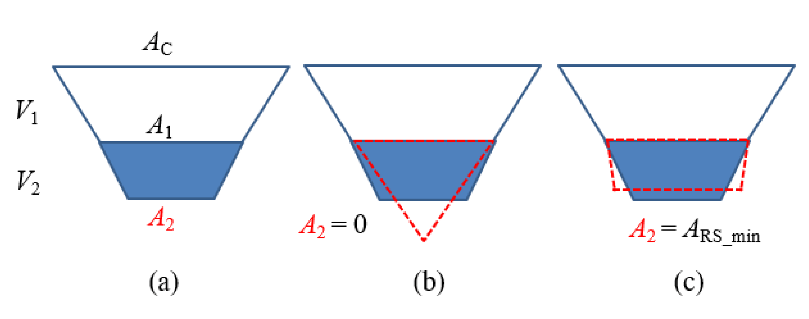
3.2.1. Surface Area Estimation

For each given reservoir, the water surface area was estimated using the enhanced K-means classification approach developed by Zhang et al. [25]. First, a threshold of 0.1 was applied to each 16-day MODIS NDVI image from 2000 to 2015, where pixels with NDVI values less than 0.1 were considered water. Based on these simplified classifications, a mask image was created to represent the water coverage percentile and to delineate the domain of the reservoir. Then, the K-means clustering algorithm [42] was used to identify all water pixels within the masked area of the MODIS NDVI images. Finally, a classification enhancement procedure was applied to finetune the results from the K-means clustering. The main purpose of the enhancement was to use the water occurrence map as a reference to correct misclassified pixels and/or to assign an appropriate class to the unclassified pixels [25].

3.2.2. Area-Elevation (A-H) Relationship Development

The SRTM DEM data were used to develop the A-H relationship for each reservoir. As a valid approximation, the relationships for all reservoirs were assumed to be linear (H = kA + b, where k is the slope of the A-H relationship, and b is the intercept) [43]. To capture the relationship, we first delineated the water surface area from the DEM for each reservoir of interest. For a given reservoir, the water surface area during the SRTM acquisition time was expanded to include its surrounding pixels by gradually increasing the surface elevation threshold, with the water surface elevation corresponding to the DEM area as the initial value. During this process, all pixels that were not directly connected to the increasing water area were discarded as noise. This expansion continued until the new area on this DEM reached the maximum reservoir area estimated from the MODIS images (from 2000 to 2015). This maximum reservoir area was then delineated from the SRTM DEM. A simplified example of a delineated reservoir is shown in Figure 3a. After delineating the maximum coverage of the reservoir from the DEM, the cumulative area (e.g., A₃) at any given elevation value (e g., H₃) could be estimated by counting the number of pixels with elevations equal to or smaller than that value (i.e., H₃). By regressing the cumulative area values against the elevation values, the A-H relationship for the reservoir of interest was established (Figure 3b). A real example of the A-H relationship development for the Pong reservoir is provided in Figure 3c,d.

An example of the A-H relationship over the Hirakud reservoir is shown in Figure 4a. This A-H relationship was also compared with that derived from MODIS area values and ICESat elevations for cross-validation purposes. The MODIS-ICESat-based A-H relationship was adopted from Zhang et al. [2014]. The A-H relationship from the MODIS-ICESat algorithm is capable of capturing a larger range of water surface elevation values due to its longer temporal coverage period (seven years). The range of elevation values associated with the SRTM based A-H relationship depends on how full the reservoir was during the SRTM flight time—the fuller the reservoir at the overpass time, the smaller the elevation range above the water. The slopes for the two relationships are fairly similar with only with a small bias.

3.2.3. Storage Estimation

Reservoir storage can be estimated based on the remotely sensed water surface area and elevation using Equation (1):

$$V_{RS}=V_C-\left(A_C+A_{RS}\right)\left(H_C-H_{RS}\right)/2$$

(1)

where V_C, A_C, and H_C represent the storage, area, and water elevation at capacity, respectively. V_RS, A_RS, and H_RS are the remotely sensed storage, area, and water height at the monitoring time.

In this MODIS-SRTM algorithm, since H_RS can be calculated by applying the A-H relationship to the MODIS area estimation (i.e., A_RS), the reservoir storage is calculated through Equation (2) (which was transformed from Equation (1)).

$$V_{RS}=V_C-\left(A_C+A_{RS}\right)\left(A_C{-\mathrm{A}}_{RS}\right)k/2$$

(2)

Using the methods explained in this section, the reservoir storage was calculated for the 28 selected reservoirs in South Asia from 2000 to 2015. Using the Hirakud reservoir as an example, Figure 4b compares the time series of reservoir storage from this MODIS-SRTM algorithm with that from the MODIS-ICESat algorithm by Zhang et al. [25]. Results suggest that these two sets of storage estimations are in good agreement. However, compared with the MODIS-ICESat-based algorithm, the storage values from this study tend to be underestimated (due to the different A-H relationships). To better understand the error statistics of these two approaches, validations using gauge data were conducted and are reported on in Section 4.1.

4. Results

The MODIS-SRTM-based reservoir storage dataset was examined comprehensively from three perspectives: First, the reliability of the dataset was tested by validating the MODIS-SRTM based reservoir storage results with both in situ gauge data and the MODIS-ICESat based results. Second, the enhanced spatial coverage from this new dataset was compared with the existing reservoir storage dataset in South Asia. Third, the uncertainties associated with the algorithm and dataset were analyzed.

4.1. Validation Results

The MODIS-SRTM-based reservoir storage was validated over 11 reservoirs (

Table 2. Statistical validation results for the remotely sensed reservoir storage data obtained from the MODIS-SRTM approach.

ID	Reservoir Name	R2	Bias (%)	NRMSE (%)
01	Almatti	0.84	12.40	35.87
05	Gabdhi Sagar	0.69	6.25	15.46
06	Hirakud	0.88	−11.07	18.44
14	N. J. Sagar	0.82	2.80	27.95
15	Pong	0.88	19.25	24.52
17	Ranjit Sagar	0.47	17.77	37.69
18	Rengali	0.79	−13.43	23.81
19	Rihand	0.84	−16.22	28.69
20	R. P. Sagar	0.91	−1.79	15.00
22	Srisailam	0.90	−31.7	32.75
26	Ukai	0.81	−14.76	15.93

) where gauge observation data were available. The performance of the results was evaluated using Equations (3)–(5), which represent three statistical criteria: the coefficient of determination (R²), the relative bias (B), and the normalized root mean square error (NRMSE):

$$R^2=\frac{{\sum }_{i=1}^n\left(R{S}_i-\overline{R{S}_i}\right)\left(OB{S}_i-\overline{Obs}\right)}{\sqrt{{\sum }_{i=1}^n{\left(R{S}_i-\overline{R{S}_i}\right)}^2}\sqrt{{\sum }_{i=1}^n{\left(Ob{s}_i-\overline{Obs}\right)}^2}}$$

(3)

$$B=\frac{\overline{RS}-\overline{Obs}}{\overline{Obs}}\times 100\%$$

(4)

$$NRMSE=\frac{\sqrt{{\sum }_{i=1}^n\frac{{(R{S}_i-Ob{s}_i)}^2}{n}}}{\overline{Obs}}\times 100\%$$

(5)

where RS represents the remotely sensed results, Obs is the gauge data, i denotes the i^th record, n is the total number of data points, and $\overline{RS}$ and $\overline{Obs}$ are the average values of the remote sensing results and the gauge data, respectively.

As shown in Table 2, most of these results were highly correlated with CEA gauge observations. The R² values ranged from 0.47 to 0.91, with a mean of 0.8. The lowest R² was found over the Ranjit Sagar reservoir. This reservoir has a relatively small area (56 km² at capacity) and is very meandering with a high shoreline to area ratio, complicating the accurate estimation of the surface area from the medium spatial resolution MODIS data [9]. This multicriteria evaluation provided a comprehensive understanding of the results. Using the Srisailam reservoir as an example, its R² value was the second highest among all of the validated reservoirs, but its NRMSE was relatively large. Because the slope of the A-H relationship (k, in Equation (2)) is constant, a high R² value suggests that the area estimations are accurate. Thus, the large NRMSE was mainly caused by errors associated with the slope of the A-H relationship. Because the area error was proven to be small as indicated by the large R², the SRTM DEM was thus the primary error source for the storage results for this reservoir. Another example is the Ranjit Sagar reservoir. Although it had an extremely low R² value due to the large amount of error in the surface area estimations, the storage bias was close to those of the Pong and Rihand reservoirs, which indicates a relatively more accurate A-H relationship over this reservoir.

The performance of this algorithm was also compared with the MODIS-ICESat algorithm by Zhang et al. [25] (

Table 3. Comparison of the validation results between the MODIS-SRTM and MODIS-ICESat approaches.

		Hirakud	N.J. Sagar	Pong	Rengali	R.P. Sagar
NRSME (%)	ICESat	14.58	26.50	15.21	19.69	18.18
	SRTM	18.44	27.95	24.52	23.81	15.00
Relative Bias (%)	ICESat	−1.88	4.13	0.41	−2.63	−8.97
	SRTM	−11.07	2.80	19.25	−13.43	−1.79
R2	ICESat	0.94	0.85	0.98	0.85	0.92
	SRTM	0.88	0.82	0.88	0.79	0.91

). The remotely sensed reservoir storage data from these two algorithms were validated over five reservoirs (Hirakud, N. J. Sagar, Pong, Rengali, and R. P. Sagar) where gauge observations and A-H values were available (from both MODIS-ICESat and SRTM).

As shown in Figure 5a, both the MODIS-SRTM and MODIS-ICESat-based approaches performed well overall. The time series from these two algorithms closely matched the gauge values for reservoir storage. To highlight the differences between the DEM and ICESat based algorithms, Figure 5b compares the storage errors against the gauge observations from these two datasets. The error statistics are provided in Table 3. Among each of the five reservoirs, the NRMSE of the MODIS-SRTM algorithm ranged from 18.14% to 27.95%, with a mean value of 21.94%. The relative bias values ranged from −11.07% to 19.25%. The NRMSE of the MODIS-ICESat algorithm ranged from 14.58% to 26.50%, with a mean value of 18.83%. The bias values ranged from −8.97% to 4.41%. In terms of accuracy, the two approaches performed relatively similarly, with the MODIS-ICESat algorithm slightly better than the DEM based algorithm. For the N. J. Sagar reservoir, the NRMSE was 27.95% for the MODIS-SRTM algorithm and 26.50% for the ICESat-based algorithm. For this reservoir, the DEM results were more accurate than the ICESat results. The NRMSE was 15.00%, which was 3.18% better than the ICESat based algorithm. For the Hirakud, Pong, and R. P. Sagar reservoirs, the MODIS-ICESat algorithm showed a superior accuracy when validated against the gauge data. The higher accuracy of the MODIS-ICESat algorithm at these three reservoirs may be attributed to the higher vertical accuracy of the ICESat elevation values, and/or the longer observation period of ICESat (than the DEM, which results in a more representative A-H relationship). Because the ICESat and SRTM approaches both use the same MODIS water area values, the larger bias of storage from the SRTM DEM implies that the lower accuracy of SRTM could reduce the quality of the reservoir storage product. As stated by the authors of [44], the components of the SRTM error include baseline roll error, phase error, beam differential errors, and timing and position errors. However, the SRTM DEM errors related to terrain, timing, and position—along with the low vertical resolution (1-m intervals)—still influenced the accuracy of the A-H relationship, which led to a higher bias of the storage calculation. Overall, the MODIS-SRTM algorithm performed reasonably well.

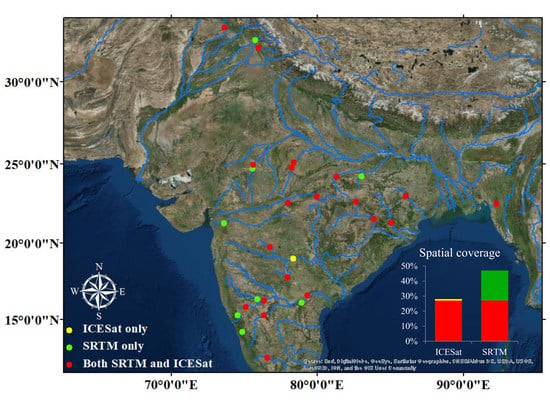
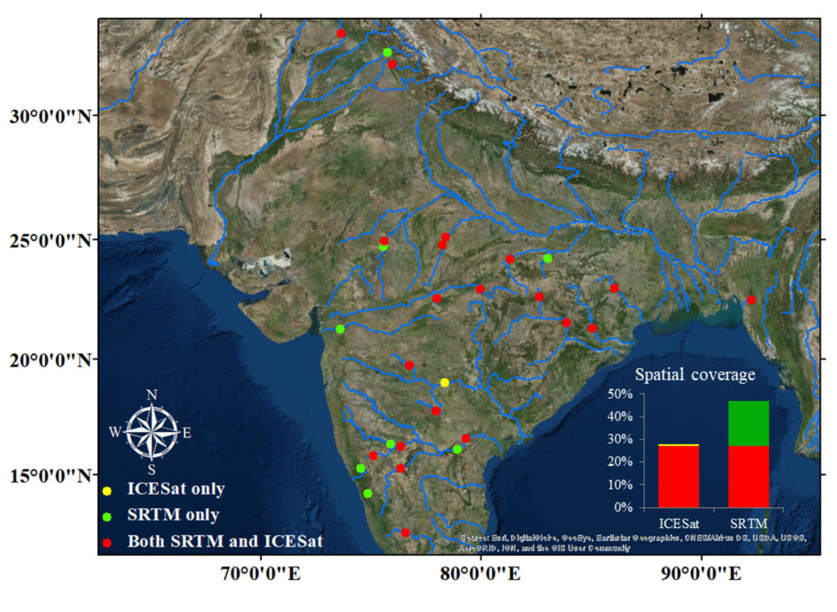
4.2. Spatial Coverage of the Reservoir Storage Dataset

With full-coverage of two-dimensional elevation data at a fine spatial resolution (30 m), the MODIS-DEM algorithm generated storage time series for the 28 reservoirs in South Asia from 2000 to 2015 (Figure 6). These reservoirs had an integrated capacity of 124.17 km³ (46.6% of the region’s total capacity). Compared with the MODIS-ICESat algorithm, the MODIS-SRTM algorithm enabled the monitoring of eight additional reservoirs (Figure 1), which represented a 18.6% increase of the overall storage capacity. Sriram Sagar, which was almost at its maximum level during the SRTM flight time, was the only reservoir for which the A-H relationship could be generated by MODIS-ICESat but not by the DEM.

The new dataset contains the storage variation information over multiple reservoirs at the basin scale, which is essential for regional water management purposes. For instance, with two additional reservoirs included in the dataset, the total storage of the monitored reservoirs in the Krishna river basin (KRB) increased from 33.4% to 67.0% (i.e., from 9.70 to 19.44 km³) of the basin’s capacity (29 km³). The Krishna River is the fourth largest river in India, with its basin extending over an area of 259,948 km² (about 8% of India). Most of the KRB is relatively flat, with about 76% of the basin covered by agricultural land. Many hydroelectric power stations are distributed along the Krishna River, providing clean energy to a large area of India. Therefore, the improved spatial representativeness of reservoirs in this river basin is essential for hydrologic modeling and water management. The Ukai Dam across the Tapti River was constructed for the purposes of irrigation, hydropower generation, and flood control. The Tapti River basin accounts for nearly two percent of the total area of India. However, before this study, no reservoir in this basin had remotely sensed elevation or storage data from space. In 2000, a severe drought occurred in the Tapti basin, causing drinking water scarcity in some villages [45]. In 2009, many districts in this basin were declared to be under drought conditions due to the deficiency of rainfall from June to September [46]. The low storage values around 2000 and 2009 (Figure 6) reflect this water scarcity. Figure 6 also shows an increase of maximum storage in the Mangla Reservoir after 2012. This is attributed to the enhanced storage capacity, that was used to increase the reservoir’s irrigation capability [47]. Another example is the Yeldari reservoir. According to media reports, two severe drought events occurred in the region in 2004 and from 2012 to 2015—and, in both cases, the Yeldari reservoir almost dried up [48,49].

4.3. Uncertainty Analysis

The storage uncertainty associated with the A-H relationship is primarily attributed to the use of partial bathymetry information to represent the A-H relationship for the entire reservoir. Because the DEM dataset only represents the part of the bathymetry that was above the water surface when the SRTM measurements were collected, it assumes that the unmeasured part below the water surface shares the same A-H relationship. To quantify the uncertainty associated with this assumption, we compared the storage estimations from three different scenarios (Figure 7). In each case, a simplified cross-sectional view of the reservoir was used—with the water surface area collected by the SRTM (in 2000) indicated as A₁, and the area of the reservoir bottom indicated as A₂. Under all scenarios, the storage volume below the DEM water surface was preserved. The first scenario (Figure 7a) follows the algorithm used in this study, which assumes that the A-H relationship remains the same across the entire profile. The second scenario (Figure 7b) assumes that the area of the reservoir bottom is zero, and thus the A-H relationship of the unknown part below the water surface has the smallest possible slope of k_min. The third scenario (Figure 7c) assumes that the minimum area from the MODIS estimations is the area of the reservoir bottom, and thus the A-H relationship of the unknown part below the water surface has the largest possible slope of k_max.

Using the slope of the upper portion (i.e., k) as estimated from the DEM, the reservoir storage value when the DEM was constructed (i.e., V₂) can be calculated using Equation (6):

$$V_2=V_c-V_1=V_c-\left(A_c+A_1\right)\left(A_c-A_1\right)k/2$$

(6)

As shown in Figure 7b, the minimum value of A₂—which is 0—can be used to estimate k_min via Equation (7):

$$k_{min}=\frac{2V_2}{\left(A_1+A_2\right)\left(A_1-A_2\right)}=\frac{2V_2}{A_1^2}$$

(7)

Similarly, the maximum value of A₂—which is equal to the minimum water surface area from MODIS during the research period (Figure 7c)—can be used to estimate k_max after Equation (8):

$$k_{max}=\frac{2V_2}{\left(A_1+A_2\right)\left(A_1-A_2\right)}=\frac{2V_2}{\left(A_1+A_{RS}^{min}\right)\left(A_1-A_{RS}^{min}\right)}$$

(8)

Thus, for any MODIS remotely sensed area (A_RS) that is less than A₁, the storage can range between a minimum possible value of V_RS^min (Equation (9)) and a maximum value of V_RS^max (Equation (10)):

$$V_{RS}^{\min }=V_2-\left(A_1+A_{RS}\right)\left(A_1-A_{RS}\right)k_{\min }/2$$

(9)

$$V_{RS}^{\max }=V_2-\left(A_1+A_{RS}\right)\left(A_1-A_{RS}\right)k_{\max }/2$$

(10)

Therefore, the uncertainties associated with the constant slope assumption can be represented by the difference between the two storage estimates described below using Equation (11):

$$∆V=\left(A_1+A_{RS}\right)\left(A_1-A_{RS}\right)\left(k_{\max }-k_{\min }\right)/2$$

(11)

The uncertainties associated with this source are illustrated in Figure 8. For all 28 reservoirs, the absolute uncertainty due to the unmeasured A-H relationship ranged from 0 km³ to 0.54 km³, with an average of 0.23 km³. Among these reservoirs, the Rihand reservoir had the largest absolute uncertainty (0.54 km³), primarily because this large reservoir was at a relatively high level when the DEM data were collected. The surface area of the Rihand reservoir—as measured by DEM—was 388.96 km², whereas its surface area at full capacity is 485 km². Considering all of the reservoirs, we found a significant increasing trend of the absolute uncertainty as the reservoir capacity increased. For every 1 km³ increase in reservoir capacity, the uncertainty increased by 0.034 km³ (p < 0.01). The averaged relative uncertainty caused by the unmeasured A-H relationship was 4.68%. However, we observed no significant relationship between the relative uncertainty and the capacity.

The uncertainties from the area estimation algorithm were quantified thoroughly by Zhang et al. [2014]. From this source, the absolute uncertainties were also found to be highly correlated with the storage at capacity, where the absolute uncertainties had an average value of 3.90%. This is a similar uncertainty range but lightly larger than the unmeasured A-H relationship.

The vertical error of SRTM DEM could be another source of uncertainty. This was not analyzed in this study because the storage calculation (in this study) was based on the slope of the A-H relationship and area estimations, rather than using the absolute elevation value from the SRTM DEM directly. Since the slope of the A-H relationship is determined by the elevation difference of reservoir pixels, the absolute vertical DEM error can be offset during the process, reducing its influence on the storage estimation.

5. Conclusions

In this study, an algorithm that leverages the SRTM DEM data was developed to improve the spatial coverage of the reservoir monitoring network in South Asia. By combining water surface area from MODIS for reservoir storage estimations, we were able to take the advantage of high temporal resolution of MODIS and large spatial coverage of SRTM. Furthermore, validation results against gauge observations over 11 reservoirs in South Asia suggested that the storage estimations had a good level of accuracy (with R² values ranging from 0.47 to 0.91). The integrated storage capacity of these reservoirs was 118.76 km³, which represents 46.6% of the overall storage in the region.

This algorithm still has some limitations that need to be noted. First, the accuracy of the proposed algorithm depends on the water level at the time the DEM data were collected. For certain reservoirs that were almost full during the SRTM acquisition time, this approach did not work. Due to the assumption that the A-H relationship derived from the DEM above the water surface represented the full bathymetry, uncertainties in storage estimations were introduced in addition to those from the area retrieval algorithm. Second, the low vertical resolution of SRTM DEM and the errors from different sources may reduce the accuracy of the storage estimation [44]. Therefore, examining the DEM errors with respect to the terrain of the reservoirs could help us to better understand the error characteristics of the storage estimation bias. Third, due to the medium resolution of MODIS, the accuracy of reservoir storage estimation decreased for the reservoir with the smallest surface area (56 km²). Nonetheless, the benefits of the extended number of reservoirs outweigh the constraints.

The algorithm proposed in this study can provide reservoir storage products that support water management on a large scale. For instance, given the long-term availability of high spatial resolution sensors, this approach could be used to monitor much smaller sized reservoirs than possible using existing techniques. This algorithm may also contribute to future satellite missions such as the Surface Water Ocean Topography (SWOT) mission, which will provide a direct water surface measurement for about two-thirds of global lakes and reservoirs, including those with an individual water area > 0.06 km².

References

1. Bai, T.; Wu, L.; Chang, J.-X.; Huang, Q. Multi-objective optimal operation model of cascade reservoirs and its application on water and sediment regulation. Water Resour. Manag. 2015, 29, 2751–2770. [Google Scholar] [CrossRef]
2. Haddeland, I.; Heinke, J.; Biemans, H.; Eisner, S.; Flörke, M.; Hanasaki, N.; Konzmann, M.; Ludwig, F.; Masaki, Y.; Schewe, J. Global water resources affected by human interventions and climate change. Proc. Natl. Acad. Sci. USA 2014, 111, 3251–3256. [Google Scholar] [CrossRef] [PubMed] [Green Version]
3. Zhao, G.; Gao, H.; Naz, B.S.; Kao, S.-C.; Voisin, N. Integrating a reservoir regulation scheme into a spatially distributed hydrological model. Adv. Water Resour. 2016, 98, 16–31. [Google Scholar] [CrossRef] [Green Version]
4. Li, Y.; Gao, H.; Jasinski, M.F.; Zhang, S.; Stoll, J.D. Deriving High-Resolution Reservoir Bathymetry From ICESat-2 Prototype Photon-Counting Lidar and Landsat Imagery. IEEE Trans. Geosci. Remote Sens. 2019, 57, 7883–7893. [Google Scholar] [CrossRef]
5. Lauri, H.; de Moel, H.; Ward, P.; Räsänen, T.; Keskinen, M.; Kummu, M. Future changes in Mekong River hydrology: Impact of climate change and reservoir operation on discharge. Hydrol. Earth Syst. Sci. 2012, 16, 4603–4619. [Google Scholar] [CrossRef]
6. Le, T.V.H.; Nguyen, H.N.; Wolanski, E.; Tran, T.C.; Haruyama, S. The combined impact on the flooding in Vietnam’s Mekong River delta of local man-made structures, sea level rise, and dams upstream in the river catchment. Estuar. Coast. Shelf Sci. 2007, 71, 110–116. [Google Scholar] [CrossRef]
7. Pulwarty, R.S.; Sivakumar, M.V. Information systems in a changing climate: Early warnings and drought risk management. Weather Clim. Extrem. 2014, 3, 14–21. [Google Scholar] [CrossRef] [Green Version]
8. Vicente-Serrano, S.M.; Beguería, S.; Gimeno, L.; Eklundh, L.; Giuliani, G.; Weston, D.; El Kenawy, A.; López-Moreno, J.I.; Nieto, R.; Ayenew, T. Challenges for drought mitigation in Africa: The potential use of geospatial data and drought information systems. Appl. Geogr. 2012, 34, 471–486. [Google Scholar] [CrossRef] [Green Version]
9. Gao, H.; Birkett, C.; Lettenmaier, D.P. Global monitoring of large reservoir storage from satellite remote sensing. Water Resour. Res. 2012, 48, W09504. [Google Scholar] [CrossRef] [Green Version]
10. Lettenmaier, D.P.; Alsdorf, D.; Dozier, J.; Huffman, G.J.; Pan, M.; Wood, E.F. Inroads of remote sensing into hydrologic science during the WRR era. Water Resour. Res. 2015, 51, 7309–7342. [Google Scholar] [CrossRef]
11. Rodrigues, L.N.; Sano, E.E.; Steenhuis, T.S.; Passo, D.P. Estimation of small reservoir storage capacities with remote sensing in the Brazilian Savannah Region. Water Resour. Manag. 2012, 26, 873–882. [Google Scholar] [CrossRef]
12. Pereira, B.; Medeiros, P.; Francke, T.; Ramalho, G.; Foerster, S.; De Araújo, J.C. Assessment of the geometry and volumes of small surface water reservoirs by remote sensing in a semi-arid region with high reservoir density. Hydrol. Sci. J. 2019, 64, 66–79. [Google Scholar] [CrossRef]
13. Zhao, G.; Gao, H. Automatic correction of contaminated images for assessment of reservoir surface area dynamics. Geophys. Res. Lett. 2018, 45, 6092–6099. [Google Scholar] [CrossRef]
14. Yao, F.; Wang, J.; Wang, C.; Crétaux, J.-F. Constructing long-term high-frequency time series of global lake and reservoir areas using Landsat imagery. Remote Sens. Environ. 2019, 232, 111210. [Google Scholar] [CrossRef]
15. Berry, P.; Garlick, J.; Freeman, J.; Mathers, E. Global inland water monitoring from multi-mission altimetry. Geophys. Res. Lett. 2005, 32. [Google Scholar] [CrossRef]
16. Birkett, C.M. Contribution of the TOPEX NASA radar altimeter to the global monitoring of large rivers and wetlands. Water Resour. Res. 1998, 34, 1223–1239. [Google Scholar] [CrossRef]
17. Wang, X.; Gong, P.; Zhao, Y.; Xu, Y.; Cheng, X.; Niu, Z.; Luo, Z.; Huang, H.; Sun, F.; Li, X. Water-level changes in China’s large lakes determined from ICESat/GLAS data. Remote Sens. Environ. 2013, 132, 131–144. [Google Scholar] [CrossRef]
18. Zhang, G.; Xie, H.; Kang, S.; Yi, D.; Ackley, S.F. Monitoring lake level changes on the Tibetan Plateau using ICESat altimetry data (2003–2009). Remote Sens. Environ. 2011, 115, 1733–1742. [Google Scholar] [CrossRef]
19. Zhang, S.; Gao, H. A novel algorithm for monitoring reservoirs under all-weather conditions at a high temporal resolution through passive microwave remote sensing. Geophys. Res. Lett. 2016, 43, 8052–8059. [Google Scholar] [CrossRef]
20. Zhang, G.; Chen, W.; Xie, H. Tibetan Plateau’s lake level and volume changes from NASA’s ICESat/ICESat-2 and Landsat missions. Geophys. Res. Lett. 2019, 46, 13107–13118. [Google Scholar] [CrossRef]
21. Liebe, J.; Van De Giesen, N.; Andreini, M. Estimation of small reservoir storage capacities in a semi-arid environment: A case study in the Upper East Region of Ghana. Phys. Chem. Earth Parts A/B/C 2005, 30, 448–454. [Google Scholar] [CrossRef]
22. Smith, L.C.; Pavelsky, T.M. Remote sensing of volumetric storage changes in lakes. Earth Surf. Processes Landf. 2009, 34, 1353–1358. [Google Scholar] [CrossRef]
23. Busker, T.; de Roo, A.; Gelati, E.; Schwatke, C.; Adamovic, M.; Bisselink, B.; Pekel, J.-F.; Cottam, A. A global lake and reservoir volume analysis using a surface water dataset and satellite altimetry. Hydrol. Earth Syst. Sci. 2019, 23, 669–690. [Google Scholar] [CrossRef] [Green Version]
24. Gao, H. Satellite remote sensing of large lakes and reservoirs: From elevation and area to storage. Wiley Interdiscip. Rev. Water 2015, 2, 147–157. [Google Scholar] [CrossRef]
25. Zhang, S.; Gao, H.; Naz, B.S. Monitoring reservoir storage in South Asia from multisatellite remote sensing. Water Resour. Res. 2014, 50, 8927–8943. [Google Scholar] [CrossRef]
26. Bonnema, M.; Hossain, F. Inferring reservoir operating patterns across the M ekong B asin using only space observations. Water Resour. Res. 2017, 53, 3791–3810. [Google Scholar] [CrossRef]
27. Tseng, K.-H.; Shum, C.; Kim, J.-W.; Wang, X.; Zhu, K.; Cheng, X. Integrating Landsat imageries and digital elevation models to infer water level change in Hoover Dam. IEEE J. Sel. Top. Appl. Earth Obs. Remote Sens. 2016, 9, 1696–1709. [Google Scholar] [CrossRef]
28. Getirana, A.; Jung, H.C.; Tseng, K.-H. Deriving three dimensional reservoir bathymetry from multi-satellite datasets. Remote Sens. Environ. 2018, 217, 366–374. [Google Scholar] [CrossRef]
29. Adhikari, P.; Hong, Y.; Douglas, K.R.; Kirschbaum, D.B.; Gourley, J.; Adler, R.; Brakenridge, G.R. A digitized global flood inventory (1998–2008): Compilation and preliminary results. Natl. Hazards 2010, 55, 405–422. [Google Scholar] [CrossRef]
30. Hydrology by Altimetry. Available online: http://www.legos.obs-mip.fr/soa/hydrologie/hydroweb/Page_2.html (accessed on 31 December 2019).
31. Global Reservoirs and Lakes Monitor. Available online: https://ipad.fas.usda.gov/cropexplorer/global_reservoir/ (accessed on 31 December 2019).
32. Goteti, G.; Famiglietti, J.S.; Asante, K. A catchment-based hydrologic and routing modeling system with explicit river channels. J. Geophys. Res. Atmos. 2008, 113. [Google Scholar] [CrossRef] [Green Version]
33. Lehner, B.; Grill, G. Global river hydrography and network routing: Baseline data and new approaches to study the world’s large river systems. Hydrol. Processes 2013, 27, 2171–2186. [Google Scholar] [CrossRef]
34. Berthier, E.; Arnaud, Y.; Vincent, C.; Remy, F. Biases of SRTM in high-mountain areas: Implications for the monitoring of glacier volume changes. Geophys. Res. Lett. 2006, 33. [Google Scholar] [CrossRef]
35. Surazakov, A.B.; Aizen, V.B. Estimating volume change of mountain glaciers using SRTM and map-based topographic data. IEEE Trans. Geosci. Remote Sens. 2006, 44, 2991–2995. [Google Scholar] [CrossRef]
36. Papa, F.; Frappart, F.; Güntner, A.; Prigent, C.; Aires, F.; Getirana, A.C.; Maurer, R. Surface freshwater storage and variability in the Amazon basin from multi-satellite observations, 1993–2007. J. Geophys. Res. Atmos. 2013, 118, 11951–11965. [Google Scholar] [CrossRef] [Green Version]
37. Rabus, B.; Eineder, M.; Roth, A.; Bamler, R. The shuttle radar topography mission—A new class of digital elevation models acquired by spaceborne radar. ISPRS J. Photogramm. Remote Sens. 2003, 57, 241–262. [Google Scholar] [CrossRef]
38. Farr, T.G.; Kobrick, M. Shuttle Radar Topography Mission produces a wealth of data. Eos Trans. Am. Geophys. Union 2000, 81, 583–585. [Google Scholar] [CrossRef]
39. U.S. Geological Survey’s Long Term Archive. Available online: https://lta.cr.usgs.gov/SRTM1Arc (accessed on 31 December 2019).
40. Indian Central Electricity Authority. Available online: http://www.cea.nic.in (accessed on 30 May 2016).
41. Lehner, B.; Liermann, C.R.; Revenga, C.; Vörösmarty, C.; Fekete, B.; Crouzet, P.; Döll, P.; Endejan, M.; Frenken, K.; Magome, J. High-resolution mapping of the world’s reservoirs and dams for sustainable river-flow management. Front. Ecol. Environ. 2011, 9, 494–502. [Google Scholar] [CrossRef] [Green Version]
42. Jain, A.K. Data clustering: 50 years beyond K-means. Pattern Recognit. Lett. 2010, 31, 651–666. [Google Scholar] [CrossRef]
43. Gao, H.; Zhang, S.; Durand, M.; Lee, H. Satellite remote sensing of lakes and wetlands. In Hydrologic Remote Sensing; CRC Press: Boca Raton, FL, USA, 2016; pp. 57–72. [Google Scholar]
44. Rodriguez, E.; Morris, C.S.; Belz, J.E. A global assessment of the SRTM performance. Photogramm. Eng. Remote Sens. 2006, 72, 249–260. [Google Scholar] [CrossRef] [Green Version]
45. Jairath, J. Droughts and Integrated Water Resource Management in South Asia: Issues, Alternatives and Futures; SAGE Publications: Southend Oaks, CA, USA, 2008. [Google Scholar]
46. India Speed. This Year’s Drought Is Severe, But Not Unprecedented. 2016. Available online: https://everylifecounts.ndtv.com/this-years-drought-is-severe-but-not-unprecedented-2230 (accessed on 31 December 2019).
47. Kayani, S.-A. Mangla Dam Raising Project (Pakistan): General Review and Socio-Spatial Impact Assessment; Hal-00719226: Islamabad, Pakistan, 2012. [Google Scholar]
48. Sud, S. 38 Reservoirs Down to 30 per Cent Storage. Rediff Business. 2004. Available online: https://www.rediff.com/money/report/water/20040728.htm (accessed on 31 December 2019).
49. Bhosale, J. You Don’t Get Water Even If You Are Ready to Pay for It. The Economic Times. 2019. Available online: https://economictimes.indiatimes.com/news/politics-and-nation/you-dont-get-water-even-if-you-are-ready-to-pay-for-it/articleshow/69066949.cms?from=mdr (accessed on 31 December 2019).
Figure 1. Locations of 28 reservoirs that can be monitored using a remote sensing approach. Yellow dots represent reservoirs that can only be monitored by the Moderate Resolution Imaging Spectroradiometer-Ice, Cloud, and Land Elevation Satellite (MODIS-ICESat). Green dots are reservoirs that can only be monitored through the MODIS-Shuttle Radar Topography Mission (STRM). Red points are reservoirs that can be monitored by both approaches. For each reservoir, detailed information is provided in Table 1.
Remotesensing 12 00745 g001
Figure 2. Flowchart of the MODIS-SRTM based reservoir storage estimation algorithm.
Remotesensing 12 00745 g002
Figure 3. (a) A simplified example of a delineated reservoir from the SRTM Digital Elevation Model (DEM), where H1 > H2 > H3 > H4; (b) the corresponding A-H relationship inferred from a simplified example; (c) real example of a delineated reservoir from the SRTM DEM over the Pong reservoir; (d) the corresponding A-H relationship inferred from the Pong reservoir.
Remotesensing 12 00745 g003
Figure 4. (a) The A-H relationship developed from SRTM compared with the relationship derived from ICESat, (b) time series of the storage estimation values for the Hirakud reservoir from both the SRTM- and the ICESat-based approaches.
Remotesensing 12 00745 g004
Figure 5. Validation results by comparing the remotely sensed storage values with gauge observations: (a) Comparison among absolute storage values; (b) comparison of storage difference (remotely sensed storage minus gauge data).
Remotesensing 12 00745 g005
Figure 6. Combined remotely sensed storage time series of the South Asian reservoirs analyzed in this study.
Remotesensing 12 00745 g006
Figure 7. Illustration of the process for quantifying the uncertainty associated with the extrapolation of the A-H relationship: (a) an example of a simplified reservoir cross section, with a bottom area of A2 identified by assuming the unmeasured portion shares the same A-H relationship, (b) the reservoir cross section by assuming the bottom area A2 is 0, (c) the reservoir cross section by assuming the reservoir bottom area A2 equals ARS_min.
Remotesensing 12 00745 g007
Figure 8. Uncertainty analysis results: (a) Absolute uncertainty; (b) relative uncertainty due to the unmeasured A-H relationship of SRTM DEM.
Remotesensing 12 00745 g008