Abstract
Radiant frost during the reproductive stage of plant growth can result in considerable wheat (Triticum aestivum L.) yield loss. Much effort has been spent to prevent and manage these losses, including post-frost remote sensing of damage. This study was done under controlled conditions to examine the effect of imposed frost stress on the spectral response of wheat plant components (heads and flag leaves). The approach used hyperspectral profiling to determine whether changes in wheat components were evident immediately after a frost (up to 5 days after frosting (DAF)). Significant differences were found between frost treatments, irrespective of DAF, in the Blue/Green (419–512 nanometers (nm)), Red (610–675 nm) and Near Infrared (NIR; 749–889 nm) regions of the electromagnetic spectrum (EMS) in head spectra, and in the Blue (415–494 nm), Red (670–687 nm) and NIR (727–889 nm) regions in the leaf spectra. Significant differences were found for an interaction between time and frost treatment in the Green (544–575 nm) and NIR (756–889 nm) in head spectra, and in the UV (394–396 nm) and Green/Red (564–641 nm) in leaf spectra. These findings were compared with spectral and temporal resolutions of commonly used field agricultural multispectral sensors to examine their potential suitability for frost damage studies at the canopy scale, based on the correspondence of their multispectral bands to the results from this laboratory-based hyperspectral study.
Keywords:
hyperspectral; frost; remote sensing; wheat; controlled environment room; Agri-sensors; REML; multispectral 1. Introduction
Field crops are exposed to a combination of abiotic stressors including extreme temperatures, changes in moisture availability, nutrient deficiencies, chemical exposure and pH imbalance [1,2]. Consequently, abiotic stress accounts for the majority of yield losses in agricultural crops worldwide [1,3,4,5]. Early identification and classification of areas under stress allows growers to more efficiently and effectively alter inputs to reduce yield penalties [6]. Several major wheat-growing regions experience Mediterranean-type climates, and, as a result, wheat (Triticum aestivum L.) is commonly sown in autumn, grows through winter and is harvested in spring as rainfall decreases and temperatures increase [7]. This phenology leaves crops vulnerable to a range of abiotic stressors particularly in the period between heading and grain-fill, with frost being of particular concern during flowering (anthesis) [8,9,10]. Exposure to frost during the reproductive phase of growth causes considerable yield loss and subsequent economic impacts to growers. For example, in Australia, it causes an estimated $360 million in direct and indirect losses per year [11,12].
Strategies for reducing the impact of frost on yield can be categorized as i) the development of frost resistant wheat varieties [13,14,15,16,17,18,19,20], ii) pre-season management strategies [7,21,22,23,24,25] and iii) post-event management of frosted crops [26]. To date, strategies for managing damage after a frost event have been restricted to grazing, cutting for hay or silage or continuing to harvest. However, the success of any post-frost management strategy relies on the ability to conduct rapid assessment of frosted areas and extent of damage in order to optimize management options, and ensure the best economic outcome.
Currently, identification of frost damage in wheat relies on visual assessment of physical symptoms in plant components (heads, leaves or stems) [10,11,27,28]. Visible signs of frost stress are generally not apparent until several days after an event, and current guidelines recommend growers assess damage between 5 and 10 days post-frost [29]. These visual methods do not allow the farmer to take advantage of valuable, non-visible information about crop health, including damage to the photosynthetic apparatus, which may be detectable in a shorter period directly following a frost event [30]. Furthermore, visible inspection may not be practical, particularly in broad-acre agriculture where fields are large, and changes in grain set, fill and growth may be too subtle to detect visually. Consequently, satellite and drone-deployed multispectral sensors have been identified as a potential approach for diagnosing frost damage at the paddock scale, as remote sensing techniques are currently used to assess the crop response to a variety of abiotic stressors, including nitrogen deficiencies [31,32,33,34], as well as water [32,35,36,37], salt [38] and heat stress [39,40,41].
Improvements in spatial, spectral, temporal and radiometric resolutions, alongside the availability of more affordable image acquisition and processing options, have made remote sensing an invaluable tool in the precision agriculture toolkit. However, not all multispectral sensors deployed for agricultural purposes (“Agri-sensors”) cover all common bands, or are consistent in the spectral regions used to represent the more common bands. Therefore, critical information about a stressor may be missed if an agri-sensor is selected without knowledge of the specific regions of the electromagnetic spectrum (EMS) that are indicative of impact. What remains, then, is to understand how frost or cold stress manifests as changes in the spectral response (reflected light across the electromagnetic spectrum (EMS)) of wheat plants in the days following an event in order to inform the selection of appropriate multispectral sensors for future frost stress detection studies.
Hyperspectral imaging provides an opportunity to address this gap through the capture of high-dimensional spectral reflectance data for signal interrogation. Hyperspectral imaging has been used to detect a variety of abiotic stresses [5,38,42,43,44,45,46] yet few studies appear to have used hyperspectral technology to detect frost stress in wheat plant components under controlled frost treatment conditions over time. In fact, much of the work in acquiring hyperspectral data of frosted wheat has been conducted using field trials. Field trials currently provide poor control (frosted versus non-frosted plant material) due to the unpredictable nature of frosts. Consequently, much of this work has been undertaken with limited ability to control for the timing, frequency or severity of frosts. Indeed, others [23,47] have highlighted the issues with obtaining a true control in field trials. As a result, an understanding of how frost damage affects the spectral reflectance of wheat immediately after a frost event has not been determined. A controlled environment approach addresses these limitations, and allows for a deeper understanding of spectral response after frost.
Thus, the aim of this study was to examine how frost stress manifests as changes in spectral reflectance of wheat plant components over time, under controlled conditions. This was done to control for the intractability of frost related field-based experiments. To address this aim, three questions were investigated: 1) do wheat plant components (heads and flag-leaves) show a spectral response (change in reflection) to frost, 2) is the spectral response the same in both heads and leaves and 3) does the spectral response change over time after frost impact? Treated (frosted) and control (non-frosted) plant components were imaged using a hyperspectral linescanner in a darkroom over a 5-day period after frost treatment in a controlled environment room. Results were then compared with current multispectral agri-sensors for potential in-field frost damage identification. Consequently, this work attempts to bridge the spectral knowledge gap outlined previously; namely, to identify regions of the EMS that are useful for identifying frost damage in wheat in a controlled environment. The approach taken proves one of the first to investigate the impact of frost over time on spectral response, using controlled conditions with frosted and non-frosted plants. This approach of spectral profiling allows for informed sensor selection, and is also applicable to other biotic or abiotic stressors.
2. Materials and Methods
To examine whether frost stress affects spectral properties of wheat plant components soon after an event, an experiment was devised to measure spectral reflectance (R) of frosted and control plants in the days after an event. Four similar glasshouse experiments were carried out. Each experiment had 4 replications (of 8 plants) with 2 factors; frost treatment (frost and control) and days after frost (DAF 1, 3 and 5—with DAF 1 being the day the plants came out of the controlled environment room (CER)). Six heads and six flag-leaves (i.e., plant components) per plant were imaged, resulting in a total of 48 components (24 × heads, 24 × leaves) per cohort for each treatment.
2.1. Glasshouse Setup
A relatively frost susceptible and widely planted wheat variety, (Triticum aestivum L. cv. Wyalkatchem) [48] was grown in pots (4.5 L) on benches in a glasshouse at the Plant Growth Facility at The University of Western Australia (UWA), Perth (31.9801° S, 115.8179° E). A standard potting mix was used consisting of 25% peat moss, 25% sand and 50% mulched pine bark. A total of 62 pots were planted at four staggered intervals, for the four cohorts of plants, between 10th and 24th April 2017. Three seeds were planted per plot, and thinned at the 3-leaf stage to leave one plant. All pots were fully randomized and arranged within the glasshouse during the growing season (April–June; average of 25 °C day and 15 °C night temperature). Pots were fertilized weekly using 1 g of Scotts Cal-Mg Grower® plus TM soluble fertilizer per pot (N 19% (NH2 15%, NH4 1.9%, NO3 2.1%), P 8%, K 16%, Mg 1.2%, S 3.8%, Fe 400 mg kg−1, Mn 200 mg kg−1, Zn 200 mg kg−1, Cu 100 mg kg−1, B 100 mg kg−1 and Mo 10 mg kg−1). An automated drip-irrigation system watered pots every 6 h to field capacity. A systemic fungicide and insecticide were applied at the 3-leaf stage and again four weeks later, for the control of common pathogenic fungi and glasshouse insect pests. Plants were kept in the glasshouse until anthesis, when half were moved to the CER for frost treatment, with the control plants remaining in the glasshouse.
2.2. Controlled Environment Room (CER) Setup and Deployment
Eight flowering plants were randomly selected per cohort (four control plants, i.e., kept in ambient conditions in the glasshouse, four treatment plants, i.e., exposed to controlled freezing conditions overnight in the CER). Six tillers with heads in the upper “canopy” were tagged per plant to ensure repeated measurement of the same components across DAFs. For each experiment, frost treated plants were transported to the CER for the duration of the frost event (overnight). The CER was comprised of two benches (2 m l × 1.5 m w × 0.7 m h), temperature control vents (convective), concrete flooring and a temperature logger suspended from the ceiling between the benches. The challenges of using CERs for the application of frost or freezing analogous with field conditions have been widely examined [20,49,50,51]. Efforts have been made to design a CER that replicates a more true radiant frost [52,53]. Recent studies have identified similarities in ice nucleation and propagation between controlled and field freezing events [51]. However, challenges in overcoming the variability of frost events in a field setting [20] have meant that CERs remain an important mechanism for exploratory analysis. Accordingly, following an iterative testing process, a protocol was developed to simulate a frost temperature profile representative of an in-field frost (Figure 1). A rectangular frame covered with plastic (a ‘canopy cover’) was constructed on each bench to both minimize the dehydration effect on the plants of air blowing into the room, and to simulate the still conditions experienced during a frost [20,52]. Water drums were placed in the CER to increase relative humidity [52]. Plant pots were ‘bubble wrapped’ for insulation in order to prevent root freezing, then placed under the canopy for frosting. Temperature loggers (TinyTag, Gemini Data Loggers Ltd, Chichester, UK) were placed under the cover within the plant canopy. Plants were returned to the glasshouse the following morning (DAF 1). Plant components were imaged at DAF 1, 3 and 5. The experiment was repeated 4 times (22–23 June, 27–28 June, 18–19 July and 26–27 July 2017).
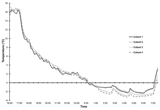
Figure 1.
Temperature at one-minute intervals for Cohorts 1–4 recorded by TinyTag® temperature loggers mounted at plant head height under the canopy cover for the duration of each event.
All frosted plant cohorts experienced temperatures below −2 °C for a number of hours (Figure 1). Cold sums in degree hours (°C.hr) per cohort were as follows: 9.9 °C.hr (Cohort 1), 9.4 °C.hr (Cohort 2), 14.1 °C.hr (Cohort 3) and 16.4 °C.hr (Cohort 4). Minimum temperatures in the CER were −2.39 °C (Cohort 1), −2.25 °C (Cohort 2), −2.99 °C (Cohort 3) and −3.27 °C (Cohort 4). The mean minimum temperature experienced in the glasshouse (control plants) was 9.04 °C (zero cold-sum hours).
2.3. Hyperspectral Image Acquisition of Wheat Plant Components
Hyperspectral sampling of plant components was conducted in a darkroom at UWA using the Pika IIi (Resonon Inc., Bozeman, MT, USA) hyperspectral linescanner (12-bit *.bil hyperspectral cubes, 240 bands (R392–R889 where Ri is the reflectance at band i in nanometers—nm), spectral resolution: 2.1 nm; spatial resolution: 640 pixels × 1000 pixels; interface: Firewire (IEEE 1394b); software; Spectronon Pro; frame rate: 137 fps; focal length: 22.5 mm; exposure: automatic (7.32 ms); scanning speed: 2100 mrps). Imaging configuration was as per Nansen, Zhang [54], whereby the sensor was mounted 20 cm above target components, and artificial lighting supplied via four 15 W LED light bulbs mounted in a square formation around the lens. The lights required a 45 min warm-up time before imaging. White reflectance calibration was performed against Spectralon, and dark calibration with lens cap attached. Plant components were imaged by gently placing a tagged component (head or flag leaf) in front of the sensor. The entirety of each head was imaged, while care was taken to ensure that the central portion of each leaf was imaged. Each tagged component was repeatedly imaged at DAF 1, 3 and 5, resulting in three hyperspectral cubes per tagged component. After imaging, plants were transported back to the glasshouse. This procedure was repeated for all cohorts.
2.4. Data extraction and Analysis
Vegetation-only pixels were extracted from each hyperspectral cube by thresholding Normalized Difference Vegetation Index (NDVI) [55] values (Equation (1)). For this experiment the wavelengths R656–670 (Red), and R804-818 (Near Infrared (NIR)) were utilized in the NDVI calculation, and thresholding was implemented using ArcMap™ 10.3.1 and ArcPy [56]. Mean reflectance (R) was calculated per band per plant component. Descriptive statistics were calculated using SPSS [57] to assess normality. Boxplots and interquartile ranges (IQR) were calculated for reflectance values per band per cohort per DAF in R [58]. From this, 64 outliers for heads and 86 outliers for leaves were identified as being outside the 1.5 × IQR, and removed, resulting in 511 mean spectra for heads, and 489 for leaves. There was no consistent pattern in outliers between treatments or DAF.
To assess whether changes in spectral response in wheat components were evident and where in the EMS changes occurred, a repeated measures linear mixed model, using residual maximum likelihood (REML) [59], was developed for significance testing using Genstat [60]. REML is useful when working with unbalanced datasets. A ‘Component-Level’ model was applied to head and leaf spectra separately, whereby individual heads or leaves (components) were considered as the repeated measure subject. Reflectance per band (Ri) was considered the response (dependent) variable, while treatment (two levels: Treated vs. Control) and DAF (three levels: 1, 3 and 5) were included as fixed-effect factors and, finally, cohort (i.e., the four repeat experiments), plants within cohort and subject (head or leaf) within plant replicates were considered random effects. The main-effects of the frost treatment or DAF were assessed first for significance, which was set at p ≤ 0.05. Interactions between the frost treatment and DAF were then assessed for significance, i.e., an interaction indicated difference in the frost treatment varied between DAFs. The resulting probability values (p) corresponding to the Wald statistic (F) for each analysis were plotted for each of the 240 bands for each main-effect (treatment and DAF), and the interaction results.
3. Experimental Results
The predicted mean spectra for frosted and control heads and leaves over time are shown in Figure 2, where the largest differences between treatments appeared to be in the NIR region (Heads: 739–889 nm; Leaves: 741–889 nm).
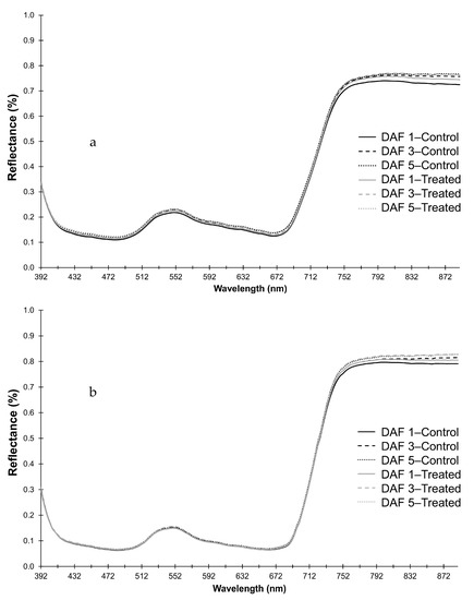
Figure 2.
Predicted mean reflectance for R392-889 for the model for (a) heads and (b) leaves for frost treated (treatment) and control plants from 1, 3 and 5 days after frost (DAF).
3.1. Effect of the Frost Treatment on Reflectance
Differences between the frost treated and control spectra were detected. There was a significant effect for frost treatment across several regions of the EMS in both head and leaf spectra (Figure 3). The highest probability of a difference due to frost for head spectra was found between R441-492 (Blue; p ≤ 0.001), with significant probabilities also found between R419–512 (Blue/Green), R610–675 (Red) and R749–889 (NIR). A distinct trough (lowest probabilities) was evident in the Red Edge (RE) region from R708-722 (p = 0.706–0.809).
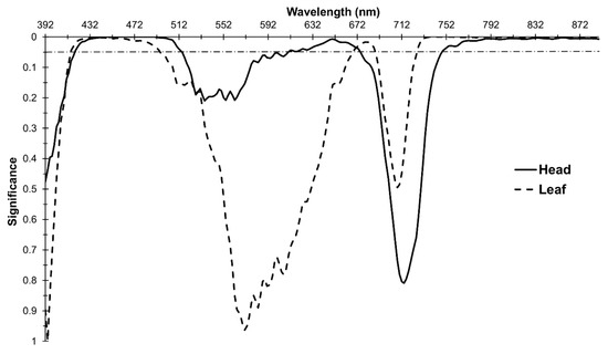
Figure 3.
Probabilities corresponding to the impact of the frost treatment as a main effect on reflectance. Horizontal dashed line is at p = 0.05.
Significant probabilities were found in similar regions of the EMS in the leaf spectral analysis (Figure 3). The highest probabilities were found between R735–776, R781–864 and R868–883 (NIR; p ≤ 0.001), with significant probabilities (p ≤ 0.05) also found between R415–494, R670–687 and R727–889.
3.2. Effect of DAF on Reflectance
Evidence of a significant response to DAF as a main effect was present across all bands for head components, and most bands for leaf components. In the analysis of head spectra, the lowest p value was 0.002 at R398 and R400, but p ≤ 0.001 for all other bands. Similarly for leaf spectra, a significant effect (p ≤ 0.05) was found across all bands excepting one, R406 (p = 0.065). Consequently, significant changes in spectral reflectance were detected across time.
3.3. Interaction of DAF and Treatment on Reflectance
The model revealed bands with significant interactions for reflectance in both head and leaf spectra indicating significant changes in spectral response between frost treatments over time (DAF) for both component types (Figure 4). The highest interaction probability for head spectra was found in the NIR at R885 (p = 0.011). Significant values were found elsewhere in the NIR, from R756–889 inclusive, alongside significant interactions in the Green across R544–575 (p values between 0.034 and 0.049; Figure 4).
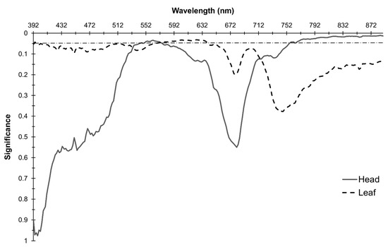
Figure 4.
Probabilities corresponding to the interaction of the frost treatment and DAF on the spectral response. Horizontal dashed line is at p = 0.05.
For leaves, the highest interaction probability was found in the Red region at two locations, R623 and R625 (p = 0.032), with significant interactions found across the Green into the Red region between R564–641 (Figure 4). Significant interactions (p ≤ 0.05) were also present in a small portion of the ultraviolet between R394–396 (Figure 4). A 10 nm window of overlap in bands with significant interactions in head and leaf spectra occurred between R564–575.
Comparing heads and leaves, bands R756–889 had both significant interactions and main effects (frost treatment and DAF) for head spectra, but this did not occur for leaf spectra (Figure 5). No interactions were found for all other bands with a significant frost treatment effect for both head and leaf spectra, thereby indicating consistent reflectance responses to frost over all DAF measured.
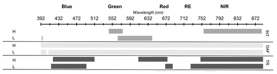
Figure 5.
Summary of bands with significant p values (p ≤ 0.05) for the interaction (INT.) and main effect of the frost treatment (TR.) and days after frost (DAF) for heads (H) and leaves (L).
Both head and leaf spectra displayed significant differences between the frost Treated and Control components in the Blue region of the EMS (Figure 5). However, heads displayed a difference in response due to the frost treatment across a broad section of the Red, while leaves displayed a difference in response in a narrow portion at the RE only (Figure 5).
The regions of the EMS where there was a significant main effect of the frost treatment and no interaction with DAF, for wheat heads, included R419–512 (Blue/Green), R610–675 (Red) and R749–754 (RE) (Figure 3, Figure 4 and Figure 5). The central band in each of these regions showed that reflectance increased in frosted plants compared with the control plants (Table 1). For leaves, the regions with a significant main effect of the frost treatment and no interaction with DAF were R415–494, R670–687 and R727–889 (Figure 3, Figure 4 and Figure 5). Again, the central band in each of these regions showed that reflectance increased in plants with the frost treatment compared with non-frosted controls (Table 1).

Table 1.
Regions of the electromagnetic spectrum (EMS) with a significant main effect of the frost treatment and DAF, with no interaction, and predicted mean reflectance of the central bands in each of these regions.
As described previously, virtually all bands had a significant DAF main effect in both heads and leaves, however, R419–542 and R576–754 for heads and R398–562 and R642–889 for leaves had no interaction with the frost treatment (Figure 5). With the exception of R392–398, with wheat heads, where reflectance increased from DAF 1 to DAF 3, then decreased from DAF 3 to DAF 5, the central bands in these regions showed that reflectance increased with time from DAF 1 to DAF 5 (Table 1).
To understand the nature of the interactions, mean reflectance spectra for the significant interactions for heads were plotted (R544–575 (Green)—Figure 6a, and R756–889 (NIR)—Figure 6b). In the Green region of the EMS, the interaction was a result of significantly higher reflectance in the frost treated heads compared with the control on DAF 1, with no differences on DAFs 3 and 5 (Figure 6a). The interaction in the NIR region for heads occurred due to significantly higher reflectance in the frosted heads compared with the control heads on DAFs 1 and 3, with no difference on DAF 5 (Figure 6b).
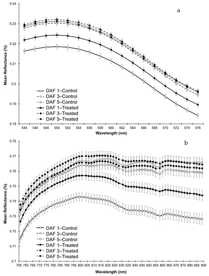
Figure 6.
Mean spectral reflectance curves with SE bars (n = 24) of head components across bands with significant interactions for (a) R544-576 (Green) and for (b) R756–889 (NIR).
For leaves, mean spectra for R394 and R396 in the ‘Purple Edge’ ((PE), R380–420), and for R564–641 (Green/ Red) were plotted (Figure 7a,b). In the PE region of the EMS the interaction was a result of significantly lower reflectance in the frost treated leaves compared with control leaves on DAF 1, with reflectance in the frosted leaves becoming significantly higher on DAF 3, with no differences on DAF 5 (Figure 7a). In the Green/Red region, the interaction was a result of a significantly higher reflectance in frosted compared with control leaves on DAF 3, with no significant differences on the other measurement dates (Figure 7b).
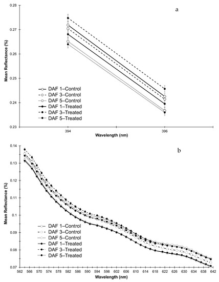
Figure 7.
Mean spectral reflectance curves with SE bars (n = 24) of leaf components across bands with significant interactions for (a) R394–396 (PE) and (b) R564–641 (Green/Red).
3.4. Selecting an Appropriate Agri-sensor for Frost-stress Detection
Many ‘off-the-shelf’ ground or drone-deployed sensors, and existing commercial satellite sensors, have pre-determined spectral resolutions (Figure 8). These bands may not be appropriate for frost-stress detection. For example, hand-held sensors, such as the Greenseeker® or Fieldscout® CM 1000, often used by growers for assessing crop vigor, make use of narrow RE bands, analogous to the NDVI (Figure 8); but more work is required to determine whether NDVI is an appropriate index for the determination of frost stress. Satellite sensors can have more than 10, sometimes contiguous, bands, and often include bands in the PE and/or Blue portion of the EMS (Figure 8). However, these bands cover broader spectral ranges (30–100 nm), and this lack of spectral granularity may not be suitable to detect subtle, narrow-band frost signals.
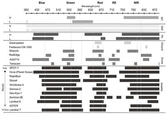
Figure 8.
Comparison of bands with significant p values (p ≤ 0.05), for interactions (INT.) and main effects of days after frost (DAF) and frost treatment (TR.) with bands covered by common ground-, drone- or satellite-deployed sensors. Vertical dashed lines are approximate centers of significant “regions” for frost stress as identified in this study. H = head and L = leaf.
This study used laboratory-acquired, component-level, hyperspectral images to identify spectral differences between frosted and non-frosted plants directly after frosting (DAF 1, 3 and 5). This laboratory-based, hyperspectral approach enabled interrogation of narrow-band spectra for signal detection, while controlling for frost event frequency and severity. Bands in regions of the EMS typically used for stress detection in vegetation were identified (Green, Red, RE and NIR), in addition to regions in the Blue, at bandwidths from approximately 17–80 nm in the RGB, and 133–162 nm in the NIR. These are bands and bandwidths similar to those used by many agri-sensors (Figure 8). While more work is required to determine whether similar spectral response is experienced under natural frost conditions, these results are promising for multispectral sensor deployment for canopy-scale studies.
In addition, it is important to determine the spatial and temporal scales at which to best capture spectral information. This study assessed ‘pure’ mean spectral reflectance per component, captured 20 cm above the target feature (head and leaf), from DAF 1 to DAF 5. Spectroradiometers are typically deployed at 1 m above canopy; while drone deployed sensors usually capture data from 15 to 120 m above canopy. The sensor distance to target, field of view (FOV) and ground sampling distance (GSD) will all affect the received spectral signal, with spectral scans or pixels containing the response of a mixture of features. In addition, the spectral signatures of crop canopies are a complex combination reflectances due to canopy structure (including leaf area, density and angle), percentage ground cover, soil background, shadow, time of day and environmental conditions. Thus, mean at-leaf or at-head, spectral reflectance as measured in a laboratory may not be the primary signal captured under field conditions. Isolating a ‘frost’ signal from this mixture for comparison with laboratory results may require spectral unmixing processes [47], particularly where full canopy closure is lacking. In addition, the identification of the most useful ‘vertical transect’ (height above target) for each spectral data capture method will also need to be identified.
Our results also indicate that detection of a spectral response to frost was possible as early as DAF 1. While hand-held, proximal sensors provided temporal flexibility, the temporal resolution (revisit times) of a satellite-based sensor could vary from daily to several weeks. For example, sensors onboard GeoEye (3 days), Deimos (2 days), SPOT (daily) and the Planet Lab suite of satellites (Dove, SkySat, RapidEye; daily) had much shorter revisit periods than those onboard Sentinel-2B (5 days) or Landsat 7 or 8 (16 days). As a result, the revisit times of these sensors are potentially inhibitive as they may miss the early stress window [61]. Environmental conditions after a frost event may not always be conducive to spectral data collection, further inhibiting the use of satellite sensors. Furthermore, while the larger spatial footprint (i.e., ground sampling distance (GSD)) of commercial satellite sensors may be advantageous for broad-scale analysis of many stresses, it is not yet clear whether frost signals would be detectable at spatial resolutions typical of even high-resolution satellite sensors (1 m—Skysat), let alone medium-resolution sensors (30 m—Landsat).
Consequently, in recent years, a drone-deployed solution has become increasingly attractive. The benefits of such methods for precision agriculture have been discussed extensively [62,63], but in summary, their advantage over other methods is due to a combination of factors, namely i) the potential for flexible, timely data capture, ii) an ability to capture higher spatial and spectral resolution imagery, iii) an increasing choice of sensors, iv) lower tasking and setup costs and v) the promise of quick data-to-information turn around. Drone-deployed, multispectral agri-sensors typically employ 4–6 bands, covering the Green, Red, RE and NIR regions of the EMS and are also typically centered in regions associated with Chl sensitivity, or “greenness” sensitivity, and thus complement the spectral ranges of many hand-held sensors (Figure 8). For crop monitoring or stress-detection purposes, these bands are often sufficient but this presents a problem for frost-mapping whereby these pre-defined narrow-band agri-sensors could also allow unique frost signals to go ‘undetected’. For example, they typically do not cover Purple Edge (PE; 380–420 nm) or Blue (400–500 nm) wavelengths in which differences in frosted and non-frosted components were identified in this study.
4. Discussion
The results from this laboratory-based experiment, as outlined above, demonstrated that frost stress could alter the spectral response of wheat plant components as early as 1–5 days after the stress was applied. The effects of frost were detected in the visible (VIS; 400–700 nm) and NIR (700–889 nm) regions of the EMS before visible changes were noticeable (5–10 days after frost) [29]. Changes in spectral reflectance differed for the frost treatment and over time. There were regions of the EMS wherein the frost treatment could be identified in both heads and leaves; however, there were other regions where frost could only be identified in one or the other plant component. Generally, reflectance increased over time in both frosted and non-frosted leaves and heads, although effects could be clearly identified for some bands after frost.
Stress can cause a reduction in plant chlorophyll (Chl) content [44,64], leading to reduced photosynthetic capacity, and altered spectral response. This response is characterized by increased reflection in the VIS region of the EMS [65], with the photosynthetic pigments Chls a and b accounting for most of the absorption of incoming electromagnetic radiation (light) in this region [66]. Sensitivity to chlorophyll content change is particularly evident at wavelengths either side of the absorption minima (550 nm) and the absorption maxima (680 nm) [66,67,68,69,70,71], making these regions useful for early-stress detection. The absorption maxima at 680 nm, closely followed by a NIR minima at 700 nm creates the characteristic Red Edge (RE) inflection point typical of healthy vegetation [67]. The RE is known to move to shorter wavelengths (the “Blue-Shift”) under a variety of abiotic stresses [69,72,73,74,75,76,77,78]. Consequently, these chlorophyll sensitive bands, and/or the RE position, have resulted in many vegetation indices being formulated to diagnose changes in Chl content and/or photosynthetic capacity [77,79,80].
In this study, an increase in reflectance due to frost stress was detected in the VIS region in both wheat heads and flag-leaves from 1 to 5 days after frost, specifically in wavelengths across 415–494 nm (Blue) and close to the absorption maxima at 670–675 nm (Red). Furthermore, component-specific (i.e., head or leaf) increases in reflectance were also detected, namely across 419–512 nm (Blue/Green) and 610–675 nm (RE) in wheat heads, and 415–494 nm (Blue) and 670–687 nm (RE) in wheat leaves. Changes found in the PE region were on the fringe of the sensor’s sensing capabilities, therefore further studies using a sensor with bands centered deeper in the UV/PE region are necessary to make conclusions as to their accuracy. Other regions of the EMS also showed a change in reflectance following frost, but these were not consistent over time. These non-consistent regions include wavelengths across the absorption minima between 544 and 575 nm (Green) in wheat heads, with a difference between treatments in these bands detectable on DAF 1 only. For wheat leaves, this occurred on one side of the minima and into the Red (564–641 nm; Green/Red), with the difference between treatments in these bands only detectable on DAF 3. These results indicate that frost-related stress may be affecting the photosynthetic capacity of frosted components from DAF 1, thereby affecting reflectance in the Chl sensitive region of the VIS.
These results are comparable with other laboratory frost or freezing studies on wheat. For example, in an examination of freezing stress on wheat seedlings Wu et al. [64] found increased reflectance across 450–650 nm, as was found here. In particular, single bands at 638 nm, 682 nm, 720 nm and 768 nm were identified as useful for freezing-injury diagnosis. They further discussed the potential for hyperspectral imaging for assessing freezing damage. In addition, in a pilot study, Flower et al. [61] found changes in reflectance occurred broadly across 500–680 nm (Green–Red) in response to controlled freezing conditions.
Perry et al. [81] found differences in similar regions using portable spectrometer readings of wheat canopies in a field setting; namely, that frosted canopies had higher reflectance at 680 nm than non-frosted. Their study primarily examined the usefulness of vegetation indices based on chlorophyll absorption wavelengths for frost discrimination. They found that only one index, the Modified Chlorophyll Absorption Reflectance Index (MCARI = ((R700-R770) − 0.2(R700-R550)(R700-R670))) [82], showed consistently significant differences between frosted and non-frosted canopies over time. However, when correlating yield to index values, the performance of the same indices was inconclusive. In this same study, a drone-deployed sensor capturing spectra at 10 nm bands in the VIS and NIR (550, 660, 710, 720, 730 and 810 nm) was also used. Indices calculated using this data were inadequate at capturing differences between frosted and non-frosted areas. Likewise, Nuttall et al. [23] tested the effectiveness of vegetation indices for classifying frosted and non-frosted spectra using portable spectrometer readings, and the same drone-sensor configuration. It was found that the Photochemical Reflectance Index (PRI = (R531-R570/R531 + R570)) [83] was the most stable across component and canopy scales. In our study, changes in bands across this region were identified for wheat heads on DAF 1, and so the PRI could prove useful in discriminating frosted and non-frosted components. However, only changes in long-wave Green bands (>564 nm) were identified for leaves on DAF 3, potentially limiting the use of the PRI for classification of frosted and non-frosted leaves.
To date, it has proven challenging to acquire spectra of frosted wheat under field conditions predominantly due to the unpredictable nature of frost, the difficulty in excluding frost from parts of the field to provide a control (non-frosted area), and uncoupling the effects of multiple frost events and event severity [23,47]. In addition, post-frost conditions may not always be suited to spectral data capture. Consequently, this study focused on the capture of high-dimensional spectra over time in a controlled environment at a plant component scale to identify wavelengths impacted by frost. However, canopy scale spectra in the field are more complex than component scale due to variations in canopy architecture, growth stage and soil and atmospheric conditions. Therefore, while the bands identified here provide valuable information on potential wavelengths to identify frost stress, further work is required to determine whether the results at the component scale, as with this study, are applicable at the canopy scale under field conditions.
To that end, Fitzgerald et al. [47] recently used spectral mixture analysis (SMA), a sub-pixel classification approach, to determine whether a set of “universal” endmembers (EMs) for frost damage could be identified from spectral libraries of frosted and non-frosted wheat. They used hyperspectral (spectrometer) data captured at multiple field locations, and at multiple scales (component, plant and 1.5 m above canopy), from which seven EMs were investigated; green (canopy or leaf), dead leaf, dry soil, senescent canopy, shade, non-frosted canopy (visually identified) and frosted canopy. While they found that SMA was promising in detecting frost stress in wheat, no universal EM set was determined.
To the best of our knowledge, no study of frosted wheat spectra have detected significant differences in the Blue region of the EMS across time as were found here, where heads and leaves exposed to frost-stress experienced an increase in reflectance relative to their non-frosted counterparts. Presumably, this increase in reflectance was due to a decrease in photosynthetic capacity as found by Guendouz, Guessoum [84] in a study of Durum wheat under semi-arid conditions. In healthy vegetation, low spectral reflectance values in the Blue are typical, due to the combined absorption features of Chl and carotenoid pigments. This overlap of strong absorption features has meant that wavelengths in this region are not often used to detect Chl content change [84], in contrast to the Green and Red regions, which are often used.
However, carotenoid concentration can provide useful plant physiological information [44], for example, carotenoid concentration often increases in plants under stress [71], carotenoids are less sensitive to stress than Chls [71] and ratios of carotenoid to Chl a have been found to rise in senescing or unhealthy plants and decrease in healthy plants [71]. Changes in this Chl/carotenoid ratio can therefore be indicative of plant health [84]. Furthermore, in contrast to Chls, carotenoids do not have an absorption feature in the Red. Accordingly, indices using bands in the Blue and Red regions were developed to determine changes in this ratio, i.e., decreasing Chl content relative to carotenoid content. These include the Normalized Difference Pigment Index (NDPI = (R680 − R430/R680 + R430)) [71,85], the Simple Ratio Pigment Index (SRPI = [R430/R680]) [71] and the Structure Independent Pigment Index (SIPI = [R790 − R450/R790 + R650]) [71]. In this study, differences in reflectance between frosted and non-frosted components over time was consistently found in bands associated with these indices, providing an indication of key bands for future research.
Beyond 700 nm (NIR), structural properties, specifically scattering caused by the mesophyll cells, dominates spectral reflectance properties over chlorophyll content [75]. In this study, in leaves, the greatest differences between frosted and non-frosted leaf spectra were found in the NIR, characterized by increases in reflectance in frost treated components. In heads, differences between treatments were also found in a narrow region of the NIR (749–754 nm), but this result must be treated with caution as an interaction was found across neighboring (collinear) bands (756–889 nm), characterized by increases in reflection on DAF 1 only. The desiccation and collapse of cells during a frost has been compared to that which occurs during drought stress [86,87], accordingly, change in reflection had been expected due to freezing-induced cell dehydration caused by ice crystal growth [87,88], and/or mechanical damage to cell shape from ice crystals themselves [89]. Other studies using more severe frost application methods have found reductions in reflectance in the NIR; for example, Flower et al. [61] found reflection decreased between 730 and 740 nm. They further investigated changes of NDVI values of frosted wheat over time, with a decrease in NDVI values detected for frosted plants at 3 days after frosting. However, many studies have found that reflectance can increase across a broad swathe of the EMS from the VIS into the Short Wave Infrared (SWIR), particularly in the early stages of dehydration [65,90,91].
5. Conclusions
In this study, we evaluated the spectral response of frosted and non-frosted wheat plant components using a controlled environment hyperspectral approach. It was found changes over time in spectral reflectance in response to frost stress could be detected from 1 to 5 DAF using hyperspectral imaging. Significant differences were found between treatments over time in several regions of the EMS, namely in the Blue, Red and NIR in both wheat heads and leaves. There was also a significant interaction between time and the frost treatment, primarily in the Green and NIR in head spectra, and the Green, and Red in leaf spectra. Differences in spectral response between wheat plant components due to frost stress under controlled conditions have not been reported previously. In addition, bands in the Blue region have not been identified as of particular interest for frost stress identification in wheat. However, more work is required to up-scale from hyperspectral scanning of plant components to sensing at canopy scale. To do this, this study demonstrated that agri-sensor(s) must be capable of imaging in several, discrete portions of the EMS, including Blue wavelengths, and have a near daily revisit or deployment rate. It suggests that drone-deployed sensors might provide a potential multi-spectral avenue for future frost research as they often include bands in the locations identified here, are potentially more flexible in deployment and provide greater opportunity for carrying bespoke sensors as this knowledge base continues to expand.
Nonetheless, an understanding of how spectral reflectance changes manifest in wheat due to frost stress is emerging, and the differences found in the Blue region in this study, which have not been reported before, provide a potential avenue for future research.
Author Contributions
M.E.M. conceptualized the present study, with support from K.C.F., B.B., and J.N.C. Methodology was devised by M.E.M. and K.C.F. with support from B.B., M.E.M. carried out the experiment and conducted the subsequent analysis with statistical support from K.C.F., M.E.M. and K.C.F. created the scripts. M.E.M. drafted the manuscript, including all figures and graphical abstract, with editorial support provided by K.C.F., B.B., and J.N.C. All authors have read and agreed to the published version of the manuscript.
Funding
This research was part funded by the Grains Research Development Corporation (GRDC) National Frost Initiative, grant number “CSP00198”.
Acknowledgments
We thank the staff at the Plant Growth Facilities at UWA, in particular, Robert Creasy and Bill Piasini, who provided skills and expertise that greatly assisted this research. In addition, we thank all our colleagues in the NFI, in particular, Eileen Perry and Glenn Fitzgerald for their support and insight during this work. The lead author was supported by an Australia Government Research Training Program (RTP) award, and also a GRDC PhD top-up award.
Conflicts of Interest
The authors declare no conflict of interest.
References
- Mittler, R. Abiotic stress, the field environment and stress combination. Trends Plant Sci. 2006, 11, 15–19. [Google Scholar] [CrossRef] [PubMed]
- Kennelly, M.; O’Mara, J.; Rivard, C.; Miller, G.L.; Smith, D. Introduction to abiotic disorders in plants. Plant Health Instr. 2012. [Google Scholar] [CrossRef]
- Boyer, J.S. Plant productivity and environment. Science 1982, 218, 443–448. [Google Scholar] [CrossRef] [PubMed]
- Kumar, M. Crop plants and abiotic stresses. J. Biomol. Res. Ther. 2013, 3. [Google Scholar] [CrossRef]
- Das, B.; Mahajan, G.R.; Singh, R. Hyperspectral Remote Sensing: Use in Detecting Abiotic Stresses in Agriculture. In Advances in Crop Environment Interaction; Springer: Singapore, 2018; pp. 317–335. [Google Scholar]
- Chaerle, L.; Hagenbeek, D.; Vanrobaeys, X.; Van Der Straeten, D. Early detection of nutrient and biotic stress in Phaseolus vulgaris. Int. J. Remote Sens. 2007, 28, 3479–3492. [Google Scholar] [CrossRef]
- Zheng, B.; Chapman, S.C.; Christopher, J.T.; Frederiks, T.M.; Chenu, K. Frost trends and their estimated impact on yield in the Australian wheatbelt. J. Exp. Bot. 2015, 66, 3611–3623. [Google Scholar] [CrossRef]
- Loss, S.P. Factors affecting frost damage to wheat in Western Australia. In Department of Agriculture and Food, Western Australia, Perth. Report 6; 1987. Available online: https://researchlibrary.agric.wa.gov.au/cgi/viewcontent.cgi?article=1003&context=fc_technicalrpts (accessed on 26 November 2019).
- Whaley, J.M.; Kirby, E.J.; Spink, J.H.; Foulkes, M.J.; Sparkes, D.L. Frost damage to winter wheat in the UK: The effect of plant population density. Eur. J. Agron. 2004, 21, 105–115. [Google Scholar] [CrossRef]
- Frederiks, T.M.; Christopher, J.T.; Sutherland, M.W.; Borrell, A.K. Post-head-emergence frost in wheat and barley: Defining the problem, assessing the damage, and identifying resistance. J. Exp. Bot. 2015, 66, 3487–3498. [Google Scholar] [CrossRef]
- Barlow, K.M.; Christy, B.P.; O’Leary, G.J.; Riffkin, P.A.; Nuttall, J.G. Simulating the impact of extreme heat and frost events on wheat crop production: A review. Field Crops Res. 2015, 171, 109–119. [Google Scholar] [CrossRef]
- March, T.; Knights, S.; Biddulph, B.; Ogbonnaya, F.; Maccallum, R.; Belford, R. The GRDC National Frost Initiative. In Proceedings of the GRDC Updates, Adelaide, Australia, 10 February 2015. [Google Scholar]
- Sutka, J. Genetic studies of frost resistance in wheat. Theor. Appl. Genet. 1981, 59, 145–152. [Google Scholar] [CrossRef]
- Sutka, J. Genetic control of frost tolerance in wheat (Triticum aestivum L.). Euphytica 1994, 77, 277–282. [Google Scholar] [CrossRef]
- Sutka, J. Genes for frost resistance in wheat. Euphytica 2001, 119, 169–177. [Google Scholar] [CrossRef]
- Fowler, D.; Limin, A.; Ritchie, J. Low-temperature tolerance in cereals: Model and genetic interpretation. Crop Sci. 1999, 39, 626–633. [Google Scholar] [CrossRef]
- Thomashow, M.F. Plant cold acclimation: Freezing tolerance genes and regulatory mechanisms. Annu. Rev. Plant Biol. 1999, 50, 571–599. [Google Scholar] [CrossRef]
- Båga, M.; Chodaparambil, S.V.; Limin, A.E.; Pecar, M.; Fowler, D.B.; Chibbar, R.N. Identification of quantitative trait loci and associated candidate genes for low-temperature tolerance in cold-hardy winter wheat. Funct. Integr. Genom. 2007, 7, 53–68. [Google Scholar] [CrossRef]
- Eagles, H.A.; Wilson, J.; Cane, K.; Vallance, N.; Eastwood, R.F.; Kuchel, H.; Martin, P.J.; Trevaskis, B. Frost-tolerance genes Fr-A2 and Fr-B2 in Australian wheat and their effects on days to heading and grain yield in lower rainfall environments in southern Australia. Crop Pasture Sci. 2016, 67, 119–127. [Google Scholar] [CrossRef]
- Frederiks, T.M.; Christopher, J.T.; Harvey, G.L.; Sutherland, M.W.; Borrell, A.K. Current and emerging screening methods to identify post-head-emergence frost adaptation in wheat and barley. J. Exp. Bot. 2012, 63, 5405–5416. [Google Scholar] [CrossRef]
- Woodruff, D.R. ’WHEATMAN’ a decision support system for wheat management in subtropical Australia. Aust. J. Agr. Res. 1992, 43, 1483–1499. [Google Scholar] [CrossRef]
- Snape, J.W.; Sarma, R.; Quarrie, S.A.; Fish, L.; Galiba, G.; Sutka, J. Mapping genes for flowering time and frost tolerance in cereals using precise genetic stocks. Euphytica 2001, 120, 309–315. [Google Scholar] [CrossRef]
- Nuttall, J.G.; Perry, E.M.; Delahunty, A.J.; O’Leary, G.J.; Barlow, K.M.; Wallace, A.J. Frost response in wheat and early detection using proximal sensors. J. Agron. Crop Sci. 2019, 205, 220–234. [Google Scholar] [CrossRef]
- Jenkinson, R.; Biddulph, B. Role of stubble management on the severity and duration of frost and its impact on grain yield. In Proceedings of the Agribusines Crop Updates, Perth, Australia, 24 February 2014. [Google Scholar]
- Smith, R.; Minkey, D.; Butcher, T.; Hyde, S.; Jackson, S.; Reeves, K.; Biddulph, B. Stubble Management Recommendations And Limitations For Frost Prone Landscapes. In Proceedings of the GRDC Updates, Perth, Australia, 27 February 2017. [Google Scholar]
- Warrick, B.E.; Miller, T.D. Freeze injury on wheat. In Texas Agricultural Extension Service; The Texas A and M University System: San Angelo, TX, USA, 1999. [Google Scholar]
- Shroyer, J.P.; Mikesell, M.E.; Paulsen, G.M. Spring freeze injury to Kansas wheat. In Agricultural Experiment Station and Cooperative Extension Service; Kansas State University: Manhattan, KS, USA, March 1995. [Google Scholar]
- White, C. Cereals-Frost Identification: The Back Pocket Guide; Bulletin 4375; grains Research and Development Corporation: Canberra, Australia; Government of Western Australia Dept. Of Agriculture: Kensington, Australia, 2000. [Google Scholar]
- The Western Australian Agricultural Authority. Frost Identification Guide for Cereals; Grains Research and Development Corporation; Department of Primary Industries and Regional Development: Western Australia, Australia, 2017. [Google Scholar]
- Marcellos, H. Wheat frost injury—freezing stress and photosynthesis. Aust. J. Agr. Res. 1977, 28, 557–564. [Google Scholar] [CrossRef]
- Rodriguez, D.; Fitzgerald, G.J.; Belford, R.; Christensen, L.K. Detection of nitrogen deficiency in wheat from spectral reflectance indices and basic crop eco-physiological concepts. Aust. J. Agr. Res. 2006, 57, 781–789. [Google Scholar] [CrossRef]
- Tilling, A.K.; O’Leary, G.J.; Ferwerda, J.G.; Jones, S.D.; Fitzgerald, G.J.; Rodriguez, D.; Belford, R. Remote sensing of nitrogen and water stress in wheat. Field Crops Res. 2007, 104, 77–85. [Google Scholar] [CrossRef]
- Fitzgerald, G.; Rodriguez, D.; O’Leary, G. Measuring and predicting canopy nitrogen nutrition in wheat using a spectral index—The canopy chlorophyll content index (CCCI). Field Crop Res. 2010, 116, 318–324. [Google Scholar] [CrossRef]
- Thorp, K.R.; Wang, G.; Bronson, K.F.; Badaruddin, M.; Mon, J. Hyperspectral data mining to identify relevant canopy spectral features for estimating durum wheat growth, nitrogen status, and grain yield. Comput. Electron. Agr. 2017, 136, 1–12. [Google Scholar] [CrossRef]
- Das, B.; Sahoo, R.N.; Pargal, S.; Krishna, G.; Verma, R.; Chinnusamy, V.; Sehgal, V.K.; Gupta, V.K. Comparison of different uni- and multi-variate techniques for monitoring leaf water status as an indicator of water-deficit stress in wheat through spectroscopy. Biosyst. Eng. 2017, 160, 69–83. [Google Scholar] [CrossRef]
- Feng, W.; Qi, S.; Heng, Y.; Zhou, Y.; Wu, Y.; Liu, W.; He, L.; Li, X. Canopy Vegetation Indices from In situ Hyperspectral Data to Assess Plant Water Status of Winter Wheat under Powdery Mildew Stress. Front. Plant Sci. 2017, 8, 1219. [Google Scholar] [CrossRef]
- Mzid, N.; Todorovic, M.; Albrizio, R.; Cantore, V. Remote sensing based monitoring of durum wheat under water stress treatments. Spatial Analysis of GEOmatics. 2017. Available online: https://hal.archives-ouvertes.fr/hal-01643477 (accessed on 6 November 2019).
- Moghimi, A.; Yang, C.; Miller, M.E.; Kianian, S.; Marchetto, P. A Novel Approach to Assess Salt Stress Tolerance in Wheat Using Hyperspectral Imaging. Front. Plant Sci. 2018, 9, 1182. [Google Scholar] [CrossRef]
- Lobell, D.B.; Ortiz-Monasterio, J.I. Impacts of day versus night temperatures on spring wheat yields. Agron. J. 2007, 99, 469–477. [Google Scholar] [CrossRef]
- Duncan, J.M.; Dash, J.; Atkinson, P.M. Elucidating the impact of temperature variability and extremes on cereal croplands through remote sensing. Glob. Change Biol. 2015, 21, 1541–1551. [Google Scholar] [CrossRef]
- Kyratzis, A.C.; Skarlatos, D.P.; Menexes, G.C.; Vamvakousis, V.F.; Katsiotis, A. Assessment of vegetation indices derived by UAV imagery for durum wheat phenotyping under a water limited and heat stressed mediterranean environment. Front. Plant Sci. 2017, 8, 1114. [Google Scholar] [CrossRef] [PubMed]
- Lelong, C.C.D.; Pinet, P.C.; Poilvé, H. Hyperspectral imaging and stress mapping in agriculture: A case study on wheat in Beauce (France). Remote Sens. Environ. 1998, 66, 179–191. [Google Scholar] [CrossRef]
- Moshou, D.; Pantazi, X.E.; Kateris, D.; Gravalos, I. Water stress detection based on optical multisensor fusion with a least squares support vector machine classifier. Biosyst. Eng. 2014, 117, 15–22. [Google Scholar] [CrossRef]
- Blackburn, G.A. Hyperspectral remote sensing of plant pigments. J. Exp. Bot. 2006, 58, 855–867. [Google Scholar] [CrossRef] [PubMed]
- Zhao, D.; Reddy, K.R.; Kakani, V.G.; Reddy, V.R. Nitrogen deficiency effects on plant growth, leaf photosynthesis, and hyperspectral reflectance properties of sorghum. Eur. J. Agron. 2005, 22, 391–403. [Google Scholar] [CrossRef]
- Römer, C.; Wahabzada, M.; Ballvora, A.; Pinto, F.; Rossini, M.; Panigada, C.; Behmann, J.; Léon, J.; Thurau, C.; Bauckhage, C.; et al. Early drought stress detection in cereals: Simplex volume maximisation for hyperspectral image analysis. Funct. Plant Biol. 2012, 39, 878–890. [Google Scholar] [CrossRef]
- Fitzgerald, G.J.; Perry, E.M.; Flower, K.C.; Callow, J.N.; Boruff, B.; Delahunty, A.; Wallace, A.; Nuttall, J. Frost Damage Assessment in Wheat Using Spectral Mixture Analysis. Remote Sens-Basel. 2019, 11, 2476. [Google Scholar] [CrossRef]
- Biddulph, B.; Laws, M.; Eckermann, P.; Maccallam, R.; Leske, B.; March, T.; Eglinton, J. Preliminary ratings of wheat varieties for susceptibility to reproductive frost damage; Grains Research Development Corporation: Adelaide, Australia, 2015. [Google Scholar]
- Single, W. Studies on frost injury to wheat. II. Ice formation within the plant. Aust. J. Agr. Res. 1964, 15, 869–875. [Google Scholar] [CrossRef]
- Single, W.V.; Marcellos, H. Studies on frost injury to wheat. IV. Freezing of ears after emergence from the leaf sheath. Aust. J. Agr. Res. 1974, 25, 679–686. [Google Scholar] [CrossRef]
- Livingston, D.P.; Tuong, T.D.; Murphy, J.P.; Gusta, L.V.; Willick, I.; Wisniewski, M.E. High-definition infrared thermography of ice nucleation and propagation in wheat under natural frost conditions and controlled freezing. Planta 2018, 247, 791–806. [Google Scholar] [CrossRef]
- Marcellos, H. A plant freezing chamber with radiative and convective energy exchange. J. Agr. Eng. Res. 1981, 26, 403–408. [Google Scholar] [CrossRef]
- Fuller, M.P.; Grice, P.L. A chamber for the simulation of radiation freezing of plants. Ann. App. Biol. 1998, 133, 111–121. [Google Scholar] [CrossRef]
- Nansen, C.; Zhang, X.; Aryamanesh, N.; Yan, G. Use of variogram analysis to classify field peas with and without internal defects caused by weevil infestation. J. Food Eng. 2014, 123, 17–22. [Google Scholar] [CrossRef]
- Tucker, C.J. Red and photographic infrared linear combinations for monitoring vegetation. Remote Sens. Environ. 1979, 8, 127–150. [Google Scholar] [CrossRef]
- ESRI. ArcMap, 10.5.1.; Environmental Systems Research Institute: Redlands, CA, USA, 2018. [Google Scholar]
- IBM Corp. IBM SPSS Statistics for Windows, 25.0; IBM Corp.: Armonk, NY, USA, 2017. [Google Scholar]
- R Core Team. R: A Language and Environment for Statistical Computing, 3.5.1.; R Foundation for Statistical Computing: Vienna, Austria, 2018; Available online: https://www.R-project.org/ (accessed on 3 February 2020).
- Patterson, H.D.; Thompson, R. Recovery of inter-block information when block sizes are unequal. Biometrika 1971, 58, 545–554. [Google Scholar] [CrossRef]
- VSN International Genstat for Windows, 19th ed.; VSN International: Hempel Hempstead, UK, 2017; Available online: https://www.vsni.co.uk/ (accessed on 3 February 2020).
- Flower, K.; Boruff, B.; Nansen, C.; Jones, H.; Thompson, S.; Lacoste, C.; Murphy, M. Proof of Concept: Remote Sensing Frost-Induced Stress in Wheat Paddocks; Grains Research and Development Corporation: Canberra, Australia, 2014. [Google Scholar]
- Puri, V.; Nayyar, A.; Raja, L. Agriculture drones: A modern breakthrough in precision agriculture. J. Stat. Manag. Syst. 2017, 20, 507–518. [Google Scholar] [CrossRef]
- King, A. Technology: The Future of Agriculture. Nature 2017, 544, S21–S23. [Google Scholar] [CrossRef]
- Wu, Q.; Zhu, D.; Wang, C.; Ma, Z.; Wang, J. Diagnosis of freezing stress in wheat seedlings using hyperspectral imaging. Biosyst. Eng. 2012, 112, 253–260. [Google Scholar] [CrossRef]
- Carter, G.A. Respones of leaf spectral reflectance to plant stress. Am. J. Bot. 1993, 80, 239–243. [Google Scholar] [CrossRef]
- Xue, L.; Yang, L. Deriving leaf chlorophyll content of green-leafy vegetables from hyperspectral reflectance. ISPRS J. Photogramm. 2009, 64, 97–106. [Google Scholar] [CrossRef]
- Horler, D.N.; Dockray, M.; Barber, J.; Barringer, A.R. Red edge measurements for remotely sensing plant chlorophyll content. Adv. Space Res. 1983, 3, 273–277. [Google Scholar] [CrossRef]
- Lichtenthaler, H.K. Vegetation stress: An introduction to the stress concept in plants. J. Plant Physiol. 1996, 148, 4–14. [Google Scholar] [CrossRef]
- Gitelson, A.A.; Merzlyak, M.N. Remote estimation of chlorophyll content in higher plant leaves. Int. J. Remote Sens. 1997, 18, 2691–2697. [Google Scholar] [CrossRef]
- Hatfield, J.L.; Gitelson, A.A.; Schepers, J.S.; Walthall, C.L. Application of spectral remote sensing for agronomic decisions. Agron. J. 2008, 100, S-117. [Google Scholar] [CrossRef]
- Peñuelas, J.; Baret, F.; Filella, I. Semi-empirical indices to assess carotenoids/chlorophyll a ratio from leaf spectral reflectance. Photosynthetica 1995, 31, 221–230. [Google Scholar]
- Hoque, E.; Hutzler, P.J. Spectral blue-shift of red edge minitors damage class of beech trees. Remote Sens. Environ. 1992, 39, 81–84. [Google Scholar] [CrossRef]
- Filella, I.; Peñuelas, J. The red edge position and shape as indicators of plant chlorophyll content, biomass and hydric status. Int. J. Remote Sens. 1994, 15, 1459–1470. [Google Scholar] [CrossRef]
- Rock, B.N.; Hoshizaki, T.; Miller, J.R. Comparison of in situ and airborne spectral measurements of the blue shift associated with forest decline. Remote Sens. Environ. 1988, 24, 109–127. [Google Scholar] [CrossRef]
- Datt, B. Remote sensing of chlorophyll a, chlorophyll b, chlorophyll a+ b, and total carotenoid content in eucalyptus leaves. Remote Sens. Environ. 1998, 66, 111–121. [Google Scholar] [CrossRef]
- Gitelson, A.A.; Merzlyak, M.N.; Lichtenthaler, H.K. Detection of red edge position and chlorophyll content by reflectance measurements near 700 nm. J. Plant Physiol. 1996, 148, 501–508. [Google Scholar] [CrossRef]
- Basso, B.; Cammarano, D.; De Vita, P. Remotely sensed vegetation indices: Theory and applications for crop management. Ital. J. Agrometeorol. 2004, 1, 36–53. [Google Scholar]
- Jones, H.G. Remote Sensing of Vegetation: Principles, Techniques, and Applications; Oxford University Press: Oxford, UK, 2010. [Google Scholar]
- Verrelst, J.; Camps-Valls, G.; Muñoz-Marí, J.; Rivera, J.P.; Veroustraete, F.; Clevers, J.G.; Moreno, J. Optical remote sensing and the retrieval of terrestrial vegetation bio-geophysical properties–A review. ISPRS J. Photogramm. 2015, 108, 273–290. [Google Scholar] [CrossRef]
- Bannari, A.; Morin, D.; Bonn, F.; Huete, A.R. A review of vegetation indices. Remote Sens. Rev. 1995, 13, 95–120. [Google Scholar] [CrossRef]
- Perry, E.M.; Nuttall, J.G.; Wallace, A.J.; Fitzgerald, G.J. In-field methods for rapid detection of frost damage in Australian dryland wheat during the reproductive and grain-filling phase. Crop Pasture Sci. 2017, 68, 516–526. [Google Scholar] [CrossRef]
- Daughtry, C.S.; Walthall, C.L.; Kim, M.S.; De Colstoun, E.B.; McMurtrey, J.E., III. Estimating corn leaf chlorophyll concentration from leaf and canopy reflectance. Remote Sens. Environ. 2000, 74, 229–239. [Google Scholar] [CrossRef]
- Gamon, J.A.; Peñuelas, J.; Field, C.B. A narrow-waveband spectral index that tracks diurnal changes in photosynthetic efficiency. Remote Sens. Environ. 1992, 41, 35–44. [Google Scholar] [CrossRef]
- Guendouz, A.; Guessoum, S.; Maamari, K.; Hafsi, M. Predicting the efficiency of using the RGB (Red, Green and Blue) reflectance for estimating leaf chlorophyll content of Durum wheat (Triticum durum Desf.) genotypes under semi arid conditions. Am.-Eurasian J. Sustain. Agric. 2012, 6, 102–107. [Google Scholar]
- Peñuelas, J.; Gamon, J.A.; Fredeen, A.L.; Merino, J.; Field, C.B. Reflectance indices associated with physiological changes in nitrogen- and water-limited sunflower leaves. Remote Sens. Environ. 1994, 48, 135–146. [Google Scholar] [CrossRef]
- Burke, M.J.; Gusta, L.V.; Quamme, H.A.; Weiser, C.J.; Li, P.H. Freezing and Injury in Plants. Annu. Rev. Plant Physiol. 1976, 27, 507–528. [Google Scholar] [CrossRef]
- Pearce, R.S. Extracellular ice and cell shape in frost-stressed cereal leaves: A low-temperature scanning-electron-microscopy study. Planta 1988, 175, 313–324. [Google Scholar] [CrossRef]
- Pearce, R.S.; Ashworth, E.N. Cell shape and localisation of ice in leaves of overwintering wheat during frost stress in the field. Planta 1992, 188, 324–331. [Google Scholar] [CrossRef] [PubMed]
- Cromey, M.G.; Wright, D.S.; Boddington, H.J. Effects of frost during grain filling on wheat yield and grain structure. New-Zeal J. Crop Hort. Sci. 1998, 26, 279–290. [Google Scholar] [CrossRef]
- Seelig, H.; Hoehn, A.; Stodieck, L.S.; Klaus, D.M.; Adams III, W.W.; Emery, W.J. The assessment of leaf water content using leaf reflectance ratios in the visible, near-, and short-wave-infrared. Int. J. Remote Sens. 2008, 29, 3701–3713. [Google Scholar] [CrossRef]
- Suplick-Ploense, M.R.; Alshammary, S.F.; Qian, Y.L. Spectral Reflectance Response of Three Turfgrasses to Leaf Dehydration. Asian J. Plant Sci. 2011, 10, 67. [Google Scholar] [CrossRef][Green Version]


© 2020 by the authors. Licensee MDPI, Basel, Switzerland. This article is an open access article distributed under the terms and conditions of the Creative Commons Attribution (CC BY) license (http://creativecommons.org/licenses/by/4.0/).