Comparative Research on Deep Learning Approaches for Airplane Detection from Very High-Resolution Satellite Images

Abstract

Object detection from satellite images has been a challenging problem for many years. With the development of effective deep learning algorithms and advancement in hardware systems, higher accuracies have been achieved in the detection of various objects from very high-resolution (VHR) satellite images. This article provides a comparative evaluation of the state-of-the-art convolutional neural network (CNN)-based object detection models, which are Faster R-CNN, Single Shot Multi-box Detector (SSD), and You Look Only Once-v3 (YOLO-v3), to cope with the limited number of labeled data and to automatically detect airplanes in VHR satellite images. Data augmentation with rotation, rescaling, and cropping was applied on the test images to artificially increase the number of training data from satellite images. Moreover, a non-maximum suppression algorithm (NMS) was introduced at the end of the SSD and YOLO-v3 flows to get rid of the multiple detection occurrences near each detected object in the overlapping areas. The trained networks were applied to five independent VHR test images that cover airports and their surroundings to evaluate their performance objectively. Accuracy assessment results of the test regions proved that Faster R-CNN architecture provided the highest accuracy according to the F1 scores, average precision (AP) metrics, and visual inspection of the results. The YOLO-v3 ranked as second, with a slightly lower performance but providing a balanced trade-off between accuracy and speed. The SSD provided the lowest detection performance, but it was better in object localization. The results were also evaluated in terms of the object size and detection accuracy manner, which proved that large- and medium-sized airplanes were detected with higher accuracy.

1. Introduction

Object detection from satellite imagery has considerable importance in areas, such as defense and military applications, urban studies, airport surveillance, vessel traffic monitoring, and transportation infrastructure determination. Remote sensing images obtained from satellite sensors are much complex than computer vision images since these images are obtained from high altitudes, including interference from the atmosphere, viewpoint variation, background clutter, and illumination differences [1]. Moreover, satellite images cover larger areas (at least 10kmx10km for one image frame) and represent the complex landscape of the Earth’s surface (different land categories) with two-dimensional images with less spatial details compared to digital photographs obtained from cameras. As a result, the data size and areal coverage of satellite images are also bigger compared to natural images. In object detection studies with satellite imagery, the visual interpretation approach that benefits from experts’ knowledge for the identification of different objects/targets is still widely used. The accuracy of this approach is dependent on the level of expertise and the approach is time consuming due to the manual process [2].

Several studies have been conducted on the automatic identification of different targets, such as buildings, aircraft, ships, etc., to reduce human-induced errors and save time and effort [1,3,4]. However, the complexity of the background; differences in data acquisition geometry, topography, and illumination conditions; and the diversity of objects make automatic detection challenging for satellite images. The object detection task can be considered as a combination of two fundamental tasks, which are the classification of the objects and determination of their location on the images. Studies conducted so far have focused on improving these two tasks separately or together [1,5].

In the early studies, the majority of the studies were conducted with unsupervised methods using different attributes. For example, the scale-invariant feature transform (SIFT) key points and the graph theorem were used for building detection from panchromatic images [6]. Alternatively, a wavelet transform was utilized in ship detection from synthetic aperture radar (SAR) images [7]. However, such unsupervised methods generally provided efficient results for simple structure types, and the results were successful for a limited variety of objects. Later studies focused on supervised learning methods so that objects with different constructions could be identified with high performance from more complex scenes [8,9]. The main reason behind the more successful results with supervised learning is that the learning process during the training phase is performed with previously manually labeled samples. Before the use of convolutional neural network (CNN) structures became widespread, different supervised learning methods were utilized with handcrafted features. In previous research, a spatial sparse coding bag-of-words (BOW) model was developed for aircraft recognition through the SVM classifier and the results were better than the traditional BOW model [10]. Gabor filters with SVM were used to detect aircraft, and achieved a 91% detection rate (DR) with a 7.5% false alarm rate (FAR) [11]. A deformation model representing the relation of the roots and parts of the objects by utilizing an extracted histogram of oriented gradient (HOG) features at different scales of images was developed and trained in a discriminatory manner as a framework for object recognition using a mixed model [12]. In another study, a probabilistic latent semantic analysis model (pLSA) and a K-Nearest Neighbor (k-NN) classifier with bag-of-visual-words (BoVW) was used for landslide detection [13]. In a more recent research, visually saliency and sparse coding methods were combined to efficiently and simultaneously recognize the multi-layered targets from optical satellite images [14].

In summary, the location of objects on the image is generally determined by scanning the entire image with a sliding window approach and a classifier, which may be selected from the abovementioned methods, which does the recognition task. The classifiers trained with these methods have a low size of parameters. Therefore, scanning the entire image with small strides allows an acceptable pace at object detection.

In 2012, following the remarkable success of AlexNet’s [15] at the ImageNet Large-Scale Visual Recognition Challenge [16], the CNN architectures, which are also known as deep learning methods, have begun to be used in different image processing problems. After the evolution of AlexNet, which can be accepted as a milestone for deep learning, deeper architectures, such as visual geometry group (VGG) [17], GoogleNet [18], which came up with inception modules, and residual network (ResNet) [19], were developed and the error rate in the competition decreased gradually. Along with these advancements, researchers started to use CNN structures in object classification with satellite images [20,21,22,23,24]. Although the remote sensing images have less spatial details and complex background, these methods can achieve highly accurate results near the visual interpretation performance.

In the challenges for object detection from natural images, competitors have tended to use state-of-the-art deep learning architectures, such as PASCAL VOC (Pattern Analysis, Statistical Modelling and Computational Learning Visual Object Classes) and COCO (Common Objects in Context) as a base network with a large amount of labeled data to beat the previous results. They applied different approaches, fine-tuning the base networks and performing some modifications; not only for increasing the accuracy of the classification part of the object detection task but also for improving the localization performance.

For the classification stage of object detection, the success of deep architectures is promising, but as they include a large number of parameters, direct use of the sliding window method, which has a high computational cost, is being abandoned. New architectures, such as the R-CNN (regions with CNN features), SPP-NET (Spatial Pyramid Pooling), Fast R-CNN, and Faster R-CNN, have emerged to overcome the computational cost disadvantage of the sliding window approach. These architectures use CNN networks as a base network for classification and solve the problem of localization by creating object candidates from the image [25,26,27,28]. With these structures, high performance and high speed could be achieved in real-time applications, such as object detection from a video stream. Additionally, object proposal approaches have become more widely used in remote sensing applications, with improvements in speed and performance [29,30,31,32,33]. Detection by producing an object proposal achieved successful results, but there is a trade-off between the detection performance and processing speed according to the number of proposals produced. The number and the accuracy of the object candidates could directly affect the precision of the trained model or reduce the detection speed [34].

In recent years, You Only Look Once (YOLO) [35] and Single Shot MultiBox Detector (SSD) [36] networks, which convert the classification and localization steps of the object detection task into a regression problem, can perform object detection tasks with a single neural network structure. These new methods have also overwhelmed the object proposal techniques in major competitions, such as PASCAL VOC (Pattern Analysis, Statistical Modelling and Computational Learning Visual Object Classes) [37] and COCO (Common Objects in Context) [38], where objects are detected from natural images. However, few studies have implemented these techniques on remotely sensed images. This is mainly due to an imbalanced dataset, where there are a large number of labeled natural images for detection tasks but less for remote sensing images. In addition, unlike the natural images, some of the objects that should be detected in satellite images are represented with few numbers of pixels due to the limitations of the sensor’s spatial resolution. Moreover, the presence of a multi-perspective data set is important to obtain highly accurate detection results. Although it is not a difficult task to create multi-perspective data sets using natural images, this could be challenging with satellite sensors. This challenge could be partially overcome by using satellite images obtained with different incidence angles to account for perspective differences in the training phase. Lastly, the atmospheric conditions and sun angle should be considered for satellite images as they affect the spectral response of the objects. Cheng et al. proposed the creation of a large-sized dataset named NWPU-RESISC45 to overcome the lack of training samples that are derived from satellite images. Their network consists of 31,500 image chips related to 45 land classes and they reported an obvious improvement in scene classification by implementing this dataset on pre-trained networks [22]. Radovic et al. worked on the detection of aircraft from unmanned aerial vehicle (UAV) imageries with YOLO and achieved a 99.6% precision rate [39]. Nie et al. used SSD to detect the various sizes of ships inshore and offshore areas using a transfer-learned SSD model with 87.9% average precision and outperformed the Faster R-CNN model, which provided an 81.2% average precision [40]. Wang et al. tried two sizes of detectors (SSD300 and SSD512) with SAR images for the same purpose and achieved 92.11% and 91.89% precisions, respectively [41].

The main objective of this research was to develop a framework with a comparative evaluation of the state-of-the-art CNN-based object detection models, which are Faster R-CNN, SSD, and YOLO, to increase the speed and accuracy of the detection of aircraft objects. To increase the detection accuracy, VHR satellite images obtained from different incidence angles and atmospheric conditions were introduced into the evaluation. As mentioned above, the trained data availability for the satellite images is limited, which is an important drawback in CNN-based architectures. Thus, this research proposes the use of a pre-trained network as a base, and improves the training data by comparatively less number of samples obtained from satellite images. In addition, default bounding boxes are generated with six different aspect ratios at every feature map layer to detect objects more accurately and faster. The detection models were trained with a labeled dataset produced from satellite images with different acquisition characteristics and by the use of the transfer learning approach. The training processes were performed repeatedly with different optimization methods and hyper-parameters. Although the accuracy is very important, it must be taken into account that the framework needs to process very large-scale satellite images quickly. Thus, a detection flow was developed to use trained models in the simultaneous detection of multiple objects from satellite images with large coverage. This research aimed to significantly contribute to the CNN-based object detection field by:

- Improving the performance of state-of-the-art object detectors on the satellite image domain by improving the learning with a patched and augmented “A Large-scale Dataset for Object DeTection in Aerial Images (DOTA)” satellite dataset (transfer learning) and hyperparameter tuning.

- Providing a detection flow that includes the slide-and-detect approach and non-Maximum suppression algorithm, to enable fast and accurate detection on large-scale satellite images.

- Providing a comparative evaluation of object detection models across different object sizes and different IOUs and preform an independent evaluation with full-sized (large-scale) Pleiades satellite images that have different resolution specs than the training dataset to investigate the transferability.

2. Data and Methods

In this section, information about the used satellite images and data augmentation process are given initially. Next, a detailed description of the evaluated network architectures is provided. Lastly, the steps and parameterization of the training process are explained.

2.1. Data and Augmentation

The DOTA dataset was used for training and testing purposes. It is an open-source dataset for object detection purposes from remote sensing images. The dataset includes satellite image patches obtained from the Google Earth^© platform, and Jilin 1 (JL-1) and Gaofen 2 (GF-2) satellites. It contains 15 object categories as airplane, ship, storage tank, baseball diamond, tennis court, basketball court, ground track field, harbor, bridge, large vehicle, small vehicle, helicopter, roundabout, soccer ball field, and swimming pool. The image sizes are in the range of 800 × 800 to 4000 × 4000. In this study, airplane detection was aimed for; therefore, 1631 images that contained 5209 commercial airplane objects were selected from the dataset. The images were split to the size of 1024 × 1024 patches to train Faster R-CNN and 608 × 608 for training SSD and YOLO-v3 detectors. The spatial resolution of the images varies in range 0.11 to 2 m and they contain various orientations, aspect ratios, and pixel sizes of the objects. In addition, the images vary according to the altitude, nadir-angles of the satellites, and the illumination conditions. The selected images were separated as 90% for training and the rest for testing. The DOTA training and test sets also include different samples in terms of airplane dimensions, background complexity, and illuminance conditions. Some image patches have some cropped objects, and some examples are black and white panchromatic images. These variations in the DOTA dataset enable the trained object detection architectures to achieve a similar performance in different image conditions (Figure 1).

Moreover, independent testing was performed with five image scenes obtained from very high-resolution pan-sharpened Pleiades 1A&1B satellite images with a 0.5-m spatial resolution and four spectral channels. In this research, Red/Green/Blue (RGB) bands of the Pleiades images were used. Satellite images were acquired in different atmospheric conditions but mostly at cloudless days and at different times in daylight. Images were collected between 2015 and 2017 in different seasons except for the winter. The images contain the Istanbul Ataturk, Istanbul Sabiha Gokcen, Izmir Adnan Menderes, Ankara Esenboga, and Antalya airport districts. They cover about a 53 km² area and contain 280 commercial airplanes. Properties of the Pleiades VHR images are provided in

Table 1. Properties of Pleiades satellite images used for model construction and independent testing.

Image Area	Acquisition Date	Incidence Angle (°)	Sun Elevation Angle (°)	Surface Area (km2)
Ataturk Airport	4/13/2017	21.16	54.43	15.03
Esenboga Airport	9/27/2015	19.4	46.42	14.97
Sabiha Gokcen Airport	4/29/2017	29.77	62.28	17.93
Antalya Airport	5/3/2017	16.88	64.61	23.42
Izmir Airport	3/28/2017	21.19	52.31	8.3

.

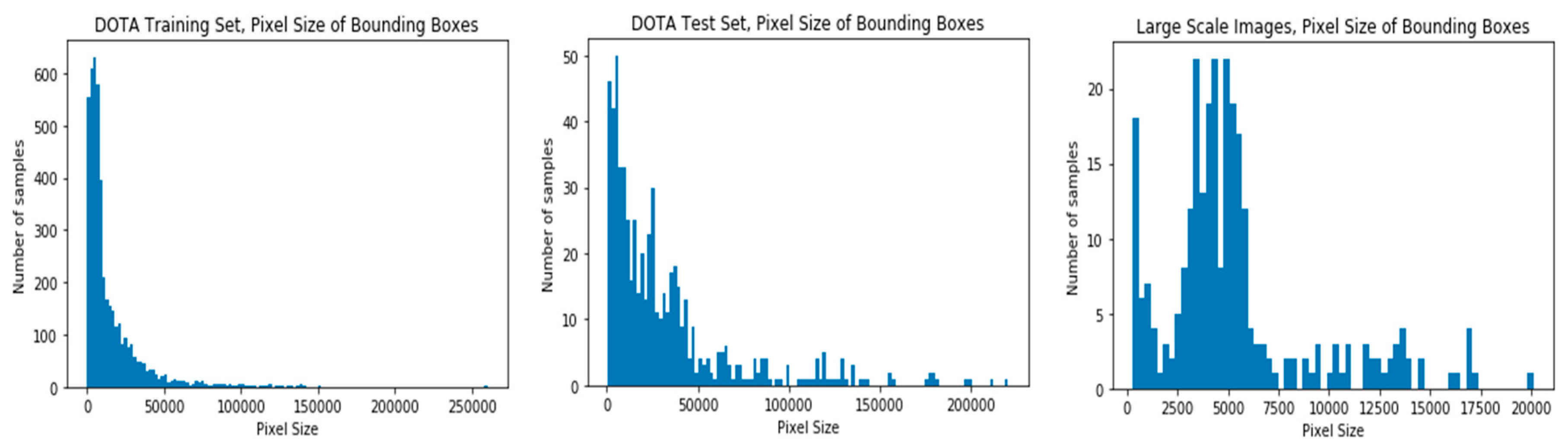
When the bounding box area distributions of aircraft samples were investigated for the DOTA training, DOTA test, and Pleiades image datasets, it was revealed that the DOTA train set includes almost the same distribution as the DOTA test set, with areas between 0 and 15,000 pixels, while it differs slightly from the samples in the large-scale Pleiades image data set. There is no object sample over 20,000 pixels in the large-scale test set and the areas of the samples are mostly between 3000 and 6000 pixels (Figure 2).

In deep architectures, a large number of labeled data is significant. Thus, the data augmentation has vital importance to cope with a lack of labeled data and to have robustness in the training step. Horizontal rotation and random cropping were applied as augmentation techniques. Besides, the image chips were scaled in HSV (hue-saturation-value) to imitate atmospheric and lighting conditions (Figure 3).

2.2. SSD Network Framework

In this sub-section, the general architecture of the SSD framework is presented initially. After, the default bounding box and negative sample generation procedures are explained. Next, the loss function and detection flow steps are presented.

2.2.1. General Architecture

The SSD is an object detector in the form of a single convolutional neural network. The SSD architecture works with the corporation of extracted feature maps and generated bounding boxes, which are called default bounding boxes. The network simply performs the loss calculation by comparing the offsets of the default bounding boxes and predicted classes with the ground truth values of the training samples at every iteration by the use of different filters. After that, it updates all the parameters according to that calculated loss value with the back propagation algorithm. In this way, it tries to learn best filter structures that can detect the features of the objects and generalize the training samples to reduce the loss value, thus attaining high accuracy at the evaluation phase [36].

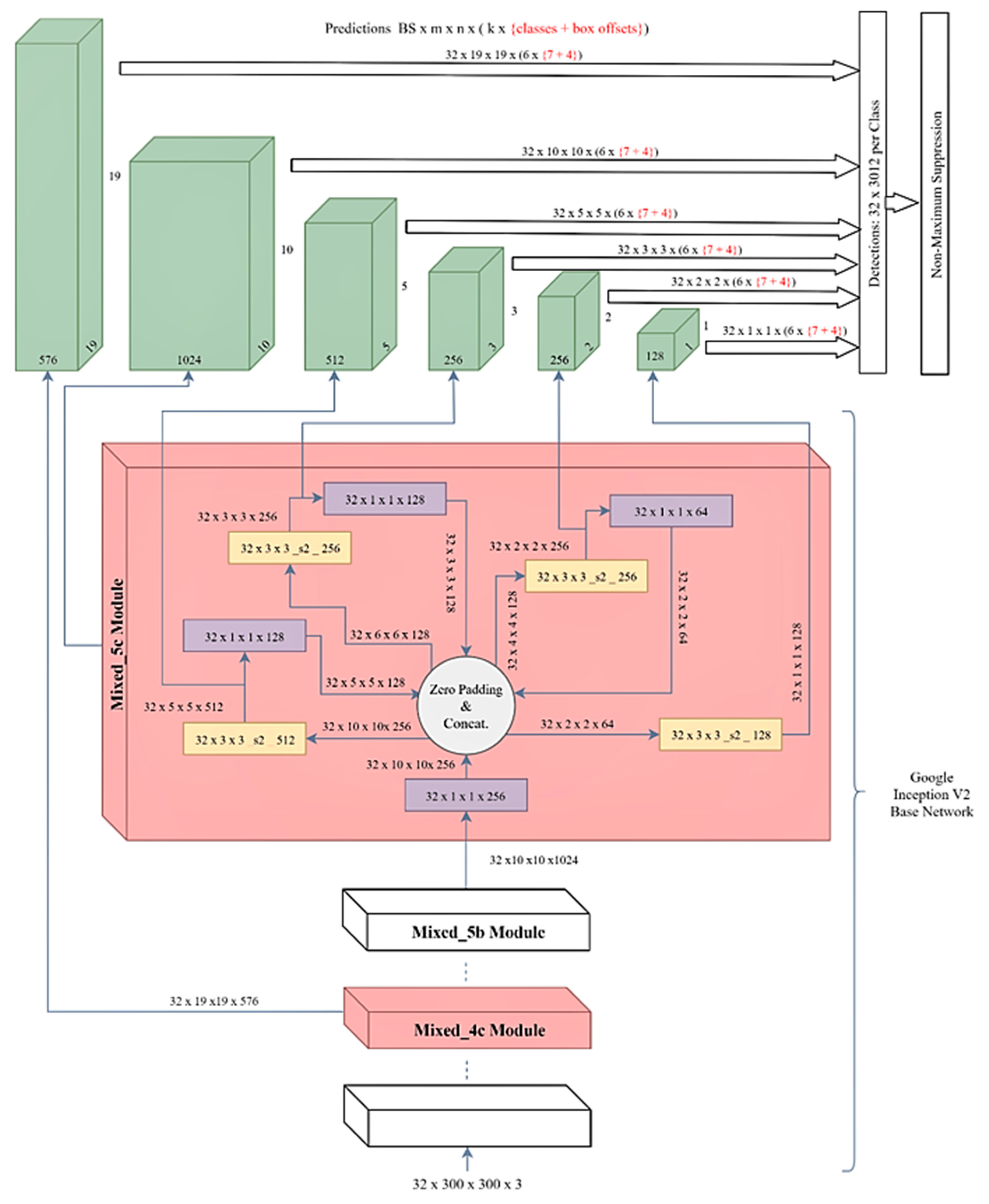
In the SSD method, a state-of-the-art CNN architecture was used as a base network for feature extraction with additional convolution layers, which produce smaller feature maps to detect the objects with different scales. Also, SSD allows more aspect ratios for generating default bounding boxes. In this way, SSD boxes can wrap around the objects in a tighter and more accurately. Lastly, the SSD network used in this research has a smaller input size, which positively affects the detection speed compared to YOLO architectures (Figure 4). Besides, YOLO has just two fully connected layers instead of additional convolution layers. These modifications are the main differences of SSD from the YOLO and they help to obtain a higher precision rate and faster detection [36].

In the original SSD research, the VGG-16 model was used as a base network. In this research, the InceptionV2 model was used to reach a higher precision and faster detection as it has a deeper structure than the VGG models. In addition, it uses fewer parameters than VGG models thanks to the inception modules that are composed of multiple connected convolution layers [42]. As an example, GoogleNet, which is one of the first networks with inception modules, employed only 5 million parameters, which represented a 12x reduction compared to AlexNet and it gives slightly more accurate results than VGG. Furthermore, VGGNet has 3x more parameters than AlexNet [18].

2.2.2. Default Bounding Boxes and Negative Sample Generation

In the initial phase of training, it is necessary to find out which default bounding box matches well with the bounding boxes of the ground truth samples. The default generated bounding boxes vary with the location and aspect ratio, and a scale process is applied by matching each ground truth box to a default box with the best jaccard overlapping value, which should be higher than 0.5 threshold. This condition facilitates the learning process and allows the network to predict high scores for multiple overlapping default boxes, rather than selecting only those that have the maximum overlap.

To handle different object scales, SSD utilizes feature maps that were extracted from several different layers in a single network. For this aim, a fixed number of default bounding boxes should be produced at different scales and aspect ratios in each region of the extracted feature maps. Six levels of aspect ratios were set supposing $a_r$ ∈ {1, 2, 3, 1/2, 1/3} and $s_k$ is the scale of the k-th square feature map for generating default boxes. The sixth one is generated for the aspect ratio of 1 with the scale of ${s^{\prime }}_k$ = $\sqrt{s_k{s}_k+1}$. Therefore, the width ($w_k^a$ = $s_k\sqrt{a_r}$) and height ($h_k^a$ = $s_k\sqrt{a_r}$) can be computed for each default box. 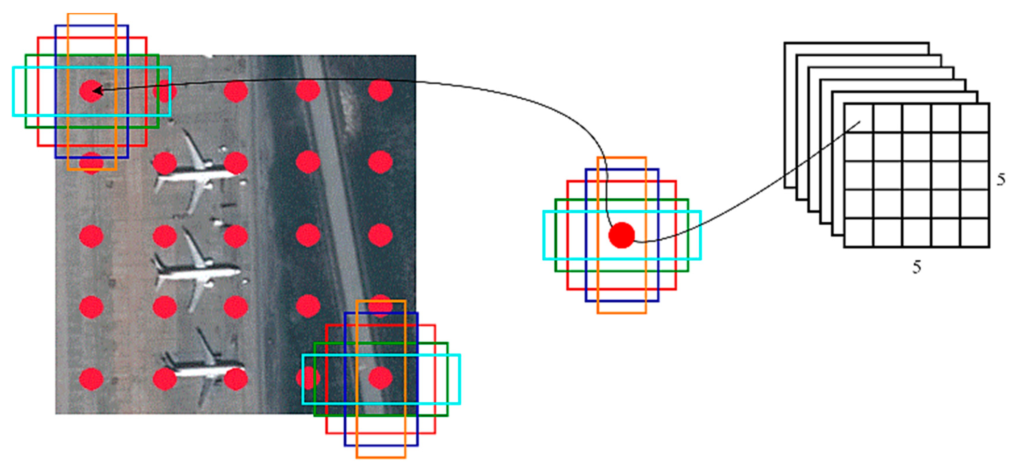Figure 3 illustrates how the generated default bounding boxes on a 5 × 5-feature map are represented on the input image and overlap with the possible objects (Figure 5). For this research, 150 bounding boxes were generated. At the same time, each of them represents the predictions in the evaluation step.

After the matching phase, which is performed at the beginning of the training, most of the default boxes are set as negatives. Instead of using all the negative examples to protect the balance with the positive examples, the confidence loss for each default box was calculated and three of them with the highest scores were selected, so the ratio between the negatives and positives is not more than 3:1. This ratio is found to provide faster optimization and training with higher accuracy [36].

2.2.3. Loss Function

The loss (objective) value was calculated as a combination of the confidence of the predicted class scores and the accuracy of the location. The total loss value (localization loss + confidence loss) given in Equation (1) is an indication of the pairing of the i-th default box with j-th ground truth box of class p, such that $x_{ij}^p=\left\{1,0\right\}$:

$$L\left(x,c,l,g\right)=\frac{1}{N}\left(L_{conf}\left(x,c\right)+\alpha L_{loc}\left(x,l,g\right)\right),$$

(1)

where N corresponds to the number of matching default boxes. If there is no match (N = 0), the total loss is determined as zero directly. The $\alpha$ value is the balance of two types of losses, and it is equal to 1 during the cross-validation phase. The localization loss is calculated as the Smooth L1 loss between the offsets of the predicted box (l) and the ground truth box (g). If the center location of the boxes denoted as cx, cy, the default boxes d, width w, and height as h:

$$L_{loc}(x,l,g)={\sum }_{i\in Po{s}_{m\in \{cx,cy,w,h\}}}^N\sum x_{ij}^{k}smoot{h}_{L1}(l_i^m-{\mathsf{ĝ}}_j^m),$$

(2)

in which:

$$smoot{h}_{L1}\left(x\right)=\{\begin{array}{cc}0.5x^2& if\left|x\right|<1\\ \left|x\right|-0.5& otherwise,\end{array}$$

$${\mathsf{ĝ}}_j^{cx}=(g_j^{cx}-d_i^{cx})/d_i^w{\mathsf{ĝ}}_j^{cy}=(g_j^{cy}-d_i^{cy})/d_i^h$$

$${\mathsf{ĝ}}_j^w=\log \frac{g_j^w}{d_i^w}{\mathsf{ĝ}}_j^h=\log \frac{g_j^h}{d_i^h}.$$

Additionally, the confidence loss (c) was calculated as a softmax loss of the predicted class relative to other classes:

$$L_{conf}\left(x,c\right)=-{\displaystyle \sum _{i\in Pos}^N}{x}_{ij}^p\log {\mathsf{ĉ}}_i^p-{\displaystyle \sum _{i\in Neg}^N}\log ({\mathsf{ĉ}}_i^0)$$

(3)

$${\mathsf{ĉ}}_i^p=\frac{\exp \left(c_i^p\right)}{{\sum }_p\exp \left(c_i^p\right)}.$$

(4)

The above-mentioned equations are detailed in Liu et al.’s article [37].

2.2.4. Detection Flow

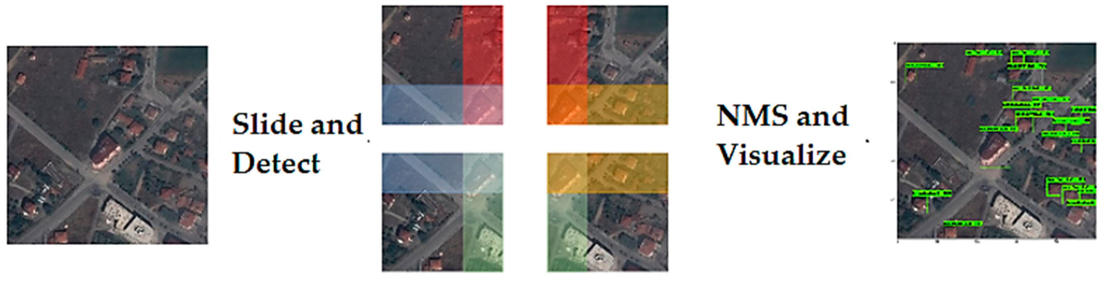
While the usual sliding window technique slides the whole image at a fixed sliding step, it cannot ensure that the windows cover the objects exactly. Moreover, small sliding steps result in huge computation costs and larger window sizes, thus decreasing the accuracy. As shown in Figure 6, a detection flow was created with the sliding window approach and an optimized sliding step to achieve higher accuracy and faster detection [43]. As an example schema, when the sliding was performed with a 300-pixel size over a 500 × 500 pixel image patch, the objects at the edges of the window could not be detected or the bounding box offsets of them would be incorrect. To tackle this problem, an overlapping area between two windows was determined as 100 pixels, which covers the object size for this research. In the sliding process for an image with a certain overlap, k × l windows were obtained to detect by the object detector for the horizontal and vertical directions, respectively:

$$k=\left[\frac{height-overlap}{ssdheight-overlap}\right],$$

(5)

$$l=\left[\frac{width-overlap}{ssdwidth-overlap}\right].$$

(6)

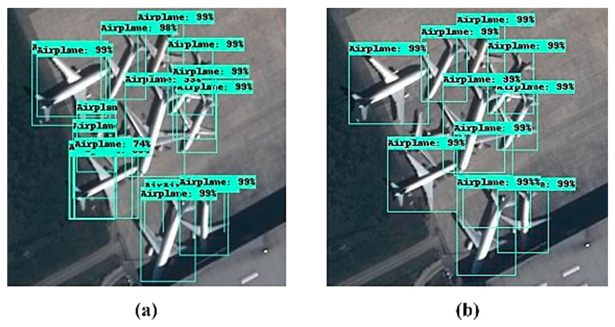
After the sliding and detection step, the non-maximum suppression (NMS) algorithm [44] (Appendix A) was used to eliminate multiple detection occurrences over an object in the overlapping regions and a score threshold was also applied to decrease the number of false detections (Figure 7).

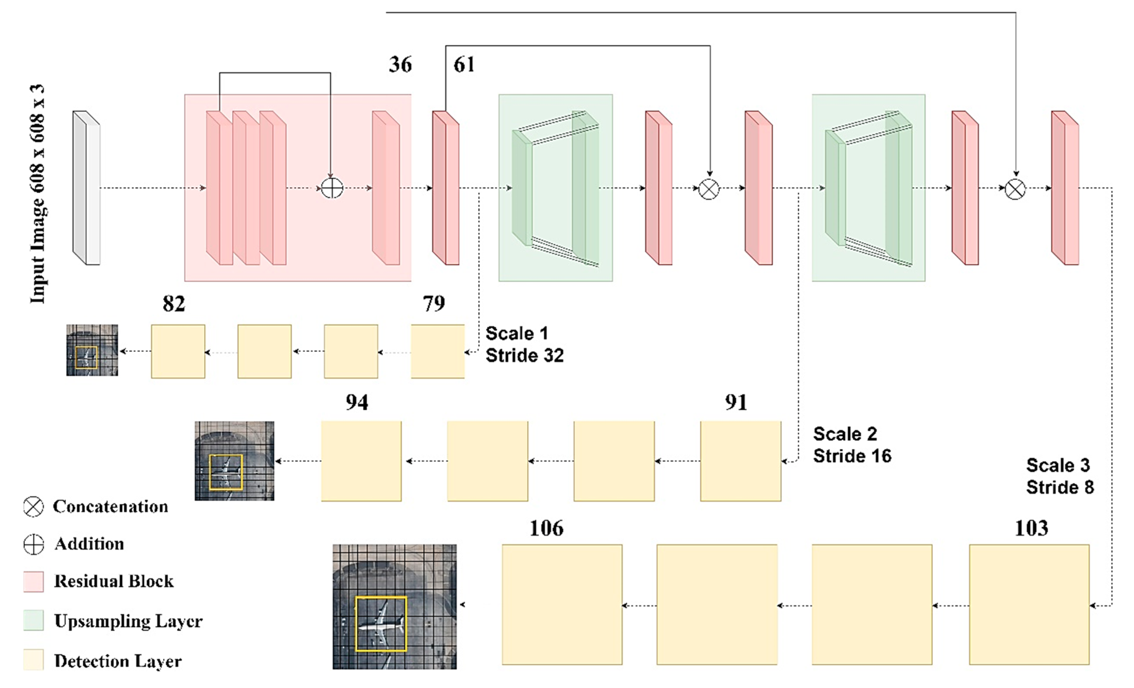
2.3. You Look Only Once (YOLO) v3 Network Framework

Yolo-v3 is grounded upon the custom CNN architecture, which is called DarkNet-53 [45]. The initial Yolo v1 architecture was inspired by GoogleNet, and it performs downsampling of the image and produces final predictions from a tensor. This tensor is obtained in a similar way as in the ROI pooling layer of the Faster R-CNN network. The next-generation Yolo v2 architecture uses a 30-layer architecture, which consists of 19 layers from Darknet-19 and an additional 11 layers adopted for object detection purposes. This new architecture provides more accurate and faster object detection results, but it often struggles with the detection of small objects in the region of interest. Moreover, it does not benefit from the advantages of the residual blocks or upsampling operations while Yolo v3 does.

Yolo v3 consists of a fully convolutional architecture, which uses a variant of Darknet, which has 53 layers trained with the Imagenet classification dataset. For the object detection tasks, an additional 53 layers were added onto it, and the improved architecture trained with the Pascal VOC dataset. With this structural design, the Yolo v3 outperformed most of the detection algorithms, while it is still fast enough for the real-time applications. With the help of the residual connections and upsampling, the architecture can perform detections at three different scales from the specific layers of the structure [45]. This makes the architecture more efficient at the detection of smaller objects but results in slower processing than the previous versions due to the complexity of the framework (Figure 8).

The shape of the detection kernel is 1 × 1 × (B × (5 + C)). In the v3 network, 3 pieces of an anchor are used for detection for each scale. Here, B is the number of the anchors on the feature map, 5 is for the 4 bounding box offsets, and one for object confidence. C is the number of categories. In the current research, the Yolo v3 network was used and the class was the only airplane, so the detection kernel shape was designed as 1 × 1 × (3 × (5 + 1)) for each scale. The first detection process was performed from the 82nd layer, as the first 81 layers downsampled the input image by the size of 32 strides. If the input image has a size of 608 × 608 pixels, that will be output as a feature map of 18 × 18 pixels in that layer. This corresponds to 18 × 18 × 18 detection features being obtained from this layer. After the first detection operation, the feature map was upsampled by a factor of 2. This upsampled feature map is was with the feature map arising from the 61st layer. Then, a few 1 × 1 convolution operations were performed to fuse features and reduce the depth dimension. After that, the second detection is performed from the 94th layer, which returns a detection feature map of 36 × 36 × 18. The same procedure was performed for the third scale at the 106th layer, which yields a feature map of the 72 × 72 × 18 size. This means it produced 20,412 predicted boxes for each image. As in the SSD network, the final predictions were proposed after the NMS algorithm was applied.

2.4. Faster R-CNN Network Framework

In this sub-section, the general architecture of the faster R-CNN framework is presented initially. After, the loss function and residual blocks are explained in detail.

2.4.1. General Architecture

Faster R-CNN is one of the most used object detection networks, which achieves accurate and quick results with CNN structures. It was initially used for nearly real-time applications, such as video indexing tasks, due to these capabilities. Faster R-CNN has developed progressively over time. The first version of it, the R-CNN, uses a selective search algorithm that utilizes a hierarchical grouping method to produce object proposals. It produces 2000 objects as the rectangular boxes, and they are passed to a pre-trained CNN model. Then, the feature maps of them are extracted from the CNN model to pass them to an SVM for classification [25].

In 2015, Girshick R. et al. [27] came up again with the Fast R-CNN, which moves the R-CNN solution one step forward. The main advantage of Fast R-CNN over the R-CNN is gained by producing the object proposals from the feature map of the CNN, instead of getting them from the complete input image. In this way, there is no need to apply the CNN process 2000 times to extract feature maps. In the next step, the region of interest (ROI) pooling is applied to ensure a standard and pre-defined output size is obtained. Finally, the future maps are classified with a softmax classifier and bounding box localizations are performed with linear regression.

In the Faster R-CNN, the selective search method is replaced by a region proposal network (RPN). This network aims to learn the proposal od an object from the feature maps. The RPN is the first stage of this object detection method. The feature maps extracted from a CNN are passed to the RPN for proposing the regions. For each location of the feature maps, k anchor boxes are used to generate region proposals. The anchor box number k is defined as 9 considering the 3 different scales and 3 aspect ratios in the original research [36]. With a size of W × H feature map, there are W × H × k anchor boxes in total, which are comprised of the negative (not object) and positive (object) samples. This means that there are many negative anchor boxes for an image, and to prevent bias occurring due to this imbalance, the negative and positive samples are chosen randomly by a 1:1 ratio (128 negative and 128 positives) as a mini-batch. The RPN learns to generate the region proposals at the training phase by utilizing these anchor boxes by comparing the ground truth boxes of the objects. The bounding box classification layer (cls) of the RPN outputs 2 × k scores whether there is an object or not for k boxes. A regression layer is used to predict the 4 × k coordinates (center coordinates of box, width, and height) of k boxes. After generation of the region proposals, the ROI pooling operation is performed as in the Fast R-CNN at the second stage of the network. Again, as in Fast R-CNN, a ROI feature vector is obtained from fully connected layers and this vector is classified by softmax to determine which category it belongs. A box regressor is applied to it to adapt the bounding box of that object. In the current research, the Faster R-CNN was used with a residual neural network (ResNet) that was comprised of 101 residual layers. This network won the COCO 2015 challenge by utilizing the ResNet-101, instead of VGG-16 in Faster R-CNN. Moreover, one additional scale parameter was added for generating the anchor boxes to detect smaller airplanes (4 scales, 3 aspect ratios, k = 12).

2.4.2. Loss Function

The loss function of the RPN network for an image was defined as:

$$L(\{p_i\},\{t_i\})=\frac{1}{N_{cls}}{\sum }_i{L}_{cls}(p_i,p_i^{\ast })+\mathsf{\lambda }\frac{1}{N_{reg}}{\sum }_i{p}_i^{\ast }{L}_{reg}\left(t_i,t_i^{\ast }\right),$$

(7)

where $i$ is the index of an anchor, $p_i$ is the prediction probability of anchor $i$ being an object, and $p_i^{\ast }$ is the ground truth label and it is 1 if the anchor is an object; otherwise, it is 0. $L_{cls}$ and $L_{reg}$ represent the classification loss, respectively, which is a log loss over two classes (object or not object) and the regression loss is the smooth $L_1$ function used for the $t_i$ and $t_i^{\ast }$ parameters. $t_i$ is a vector representation of the predicted bounding box, and $t_i^{\ast }$ is a ground truth bounding box associated with a positive anchor. Lastly, the parameter $\mathsf{\lambda }$ is used for balancing the loss function terms, and $N_{cls}$ and $N_{reg}$ are the normalization parameters of the classification and regression losses according to the mini-batch size and anchor locations.

2.4.3. Residual Blocks

When the CNN networks are designed with a deeper structure, degradation problems can occur. As the architecture becomes deeper, the layers of the higher level can act simply as an identity function. The output of them, which are the feature maps, becomes more similar to the input data. This phenomenon causes saturation in the accuracy, which is followed by fast degradation. To solve this problem, the residual blocks can be used. Instead of learning from a direct mapping of × → y with a function H(x), the residual blocks can be used to modify the function as H(x) = F(x) + x, where F(x) and × represent the stacked non-linear layers and identity function, respectively.

2.5. Training

In this work, all the experiments were performed with the Tensorflow and Keras open-source deep learning framework, which was developed by the Google research team [46]. The transfer learning technique was applied by using the pre-trained network with the COCO dataset. Additionally, fine-tuning of the parameters and extending the training set with the sample collection were performed to improve the performance as much as possible.

Through the transfer learning approach, the training was started with the implementation of the pre-trained parameters to include the useful information gathered from a previously trained network with different data used for another problem in the computer vision area. Although the COCO dataset contains natural images, the pre-trained model of the networks, which was utilized from COCO, can be used for the current research as well, because features, such as the edge, corner, shape, and color, can be implemented, which form the basis of all of the vision tasks. After starting the network with the parameters of the pre-trained model, it was fed with training examples from the produced DOTA image chips.

For Faster R-CNN, 1024 × 1024 sized image patches were used to train the model. For the RPN stage, the bounding box scales were defined as 0.25, 0.5, 1.0, and 2.0 with 0.5, 1.0, and 2.0 aspect ratios, which ensured that the network generated 12 anchor boxes for each location of the feature maps. The batch size was defined as 1 to prevent memory allocation errors. For the first attempt of the training, the process continued until 400,000 iterations, which took 72 h. The learning rate was started at 0.003 and was reduced to half of it in each further 75,000 step. The training loss did not decrease more, thus a new training process was initialized, with the learning rate corresponding to a tenth of the previous value, and the process continued for 900,000 iterations by reducing the learning rate to a quarter for each 50,000 step after the 150,000th iteration.

For the SSD network, 608 × 608-sized image patches were used for training. The sizes and aspect ratios of the default bounding boxes of each feature map layers remained the same as the original SSD research [36]. The RMSProp optimization method was used for gradient calculations with a 0.001 learning rate and 0.9 decay factor for each 25,000 iteration. The batch size was defined as 16 and the training process was continued till the 200,000th step, which took 60 h. The first attempt at the SSD training provided unsatisfactory results similar to Faster R-CNN. Therefore, a new training process initialized with a 0.0004 learning rate value and the same decay factor for each 50,000th iteration along with 450,000 iterations.

The Yolo-v3 architecture was trained with the Adam optimizer by a learning rate of 5 × 10⁻⁵ with a decay factor of 0.1 for every 3 epochs, with which the validation loss did not decrease. We used 9 anchor boxes with different sizes, 3 for each stage of the network, as in the original paper. Before the training, the bounding boxes of the entire data were clustered according to their sizes with the k-means clustering algorithm to find 9 optimum anchor box sizes. In the next step, bounding boxes were sorted from smallest to largest. For the validation purpose, 10% of the training data was split for monitoring the validation loss during the training process. The batch size was defined as 8 and the whole training was continued for 80 epochs. One epoch means the feed forward and back propagation processes are completed for the whole training dataset. Training of the Yolo-v3 took about 36 h.

3. Results and Discussion

In this section, the evaluation metrics used in this research are introduced in the first place. Secondly, the comparative results of each network according to COCO metrics across different datasets are presented and discussed. Next, the overall performance of the networks is discussed with respect to the precision, recall, and F1 scores. Lastly, a visual evaluation of the results is provided.

3.1. Evaluation Metrics

In the object detection tasks, two widely used performance metrics are the average precision (AP) and F1 score. At the training process, a detector compares the predicted bounding boxes with the ground truth bounding boxes according to the intersection over union (IOU) at each iteration to update its parameters. Generally, a 0.5 IOU ratio for each prediction at the training stage is aimed for. This means that if the network predicts an object with a bounding box that overlaps with the ground truth box by at least 50%, it is considered as a true prediction. When the localization is a matter for a computer vision task, this ratio could be set higher. In this research, the value remained as 0.5, and it was expected to detect the objects at least with this ratio at the evaluation phase. Therefore, this ratio was used for calculating the performance metrics.

The F1 score evaluation metric is used to understand the success rate by calculating the precision and recall rate. The precision is the ratio of the actual matches of all objects that are detected as matches and the recall is the ratio of the number of objects that are detected correctly to the number of all ground truth samples. Neither the recall rate nor precision rate is individually enough to measure the performance of the framework; therefore, the harmonic mean of them, which is the F1 score, was also calculated. By defining the true positive (TP) as truly detected objects, the false negative (FN) as non-detected objects, and the false positive (FP) as falsely detected objects, the precision, recall and F1 score was calculated as:

$$Precision=\frac{TP}{TP+FP},$$

(8)

$$Recall=\frac{TP}{TP+FN},$$

(9)

$$F1score=2\ast \frac{Precision\ast Recall}{Precision+Recall}.$$

(10)

Additionally, 12 different metrics were used to measure the characteristics and performance of the object detection algorithms with the COCO metric API (

Table 2. COCO performance metrics with calculation rules.

Calculated for	Metric Name
AP for [ IoU = 0.50:0.95 | area = all | maxDets = 100 ]	1. Metric
AP for [ IoU = 0.50 | area = all | maxDets = 100 ]	2. Metric
AP for [ IoU = 0.75 | area = all | maxDets = 100 ]	3. Metric
AP for [ IoU = 0.50:0.95 | area = small | maxDets = 100 ]	4. Metric
AP for [ IoU = 0.50:0.95 | area = medium | maxDets = 100 ]	5. Metric
AP for [ IoU = 0.50:0.95 | area = large | maxDets = 100 ]	6. Metric
AR for [ IoU = 0.50:0.95 | area = all | maxDets = 1 ]	7. Metric
AR for [ IoU = 0.50:0.95 | area = all | maxDets = 10 ]	8. Metric
AR for [ IoU = 0.50:0.95 | area = all | maxDets = 100 ]	9. Metric
AR for [ IoU = 0.50:0.95 | area = small | maxDets = 100 ]	10. Metric
AR for [ IoU = 0.50:0.95 | area = medium | maxDets = 100 ]	11. Metric
AR for [ IoU = 0.50:0.95 | area = large | maxDets = 100 ]	12. Metric

). Unless defined otherwise, the average precision (AP) and average recall (AR) weree calculated by averaging over 10 different IOU ranging from 0.5 to 0.95 with 0.05 intervals. Besides, the values where IOU is 0.5 and 0.75 were calculated for AP. AP is the average precision calculation according to all categories and IOU values. In this research, there was only one detection category, which is airplane. AR is the maximum number of detections per image, averaged over categories and IoUs. These calculations were also checked by interpreting the bounding box areas. According to COCO, objects with a size smaller than 32² pixels are defined as small, between 32² and 96² as medium, and more than 96² pixels as large. The metric calculations were performed according to all scale levels and for separate scales [47].

3.2. Evaluation with COCO API

The DOTA dataset was randomly divided into two as a training and test with 90% and 10% ratios, respectively. However, there is a difference in the distribution of object scales for the training and test groups. Moreover, for the independent large-scale image set produced from Pleiades satellite images, most of the objects are in the medium range (

Table 3. The ratios (%) of data sets according to the object scale.

Data Set/Object Scale	Small	Medium	Large
DOTA Training Set	0.06	0.52	0.42
DOTA Test Set	0.03	0.28	0.69
Large Scale Image Set	0.10	0.76	0.14

).

To evaluate the converge rates of the models on the training data, the performance metrics were also calculated for the DOTA training set, in addition to the test data. The performances of all trained models were examined with the COCO metric API, except for the first training attempts of SSD and Faster R-CNN as their learning rate was low (

Table 4. Performance of DOTA training, DOTA test, and large-scale image set according to COCO metrics.

	DOTA Training Set			DOTA Test Set			Large Scale Image Set
	Yolo-v3	SSD (2nd)	F RCNN (2nd)	Yolo-v3	SSD (2nd)	F RCNN (2nd)	Yolo-v3	SSD (2nd)	F RCNN (2nd)
Metric 1	0.428	0.411	0.481	0.391	0.371	0.451	0.148	0.151	0.172
Metric 2	0.806	0.711	0.757	0.76	0.618	0.717	0.434	0.431	0.364
Metric 3	0.397	0.445	0.573	0.345	0.415	0.513	0.079	0.078	0.136
Metric 4	0.044	0.020	0.119	0.077	0.040	0.088	0.055	0.026	0.046
Metric 5	0.417	0.399	0.463	0.358	0.290	0.394	0.179	0.188	0.169
Metric 6	0.491	0.475	0.540	0.414	0.422	0.485	0.060	0.146	0.300
Metric 7	0.187	0.188	0.210	0.252	0.273	0.302	0.006	0.006	0.009
Metric 8	0.482	0.458	0.515	0.458	0.431	0.501	0.069	0.056	0.073
Metric 9	0.500	0.475	0.536	0.458	0.432	0.501	0.242	0.276	0.265
Metric 10	0.064	0.067	0.167	0.075	0.087	0.138	0.052	0.078	0.074
Metric 11	0.484	0.462	0.520	0.407	0.355	0.427	0.275	0.295	0.262
Metric 12	0.568	0.536	0.596	0.487	0.471	0.539	0.198	0.305	0.408

). According to the COCO metrics, the Faster R-CNN model provided the best results when considering the mean of the precision for different IoU values. Yolo-v3 provided promising results for 0.5 IoU and above, while Faster R-CNN is better if 0.75 IOU and above is desired. For metrics 4, 5, and 6, Faster R-CNN provided the best AP result for different IOUs in small, medium, and large objects for the DOTA test set. However, in the large-scale image set, the Yolo-v3 model provided better results for small and medium objects. The reason for these results is that the architectures have different structures to learn different attributes from the training data. The seventh, eighth, and ninth metrics provide information about the recall rates for all object sizes according to the detection number per image. Similarly, the Faster R-CNN provided better results according to these metrics. When the AR results were investigated according to metrics 10, 11, and 12, it was revealed that the recall rates of Yolo-v3 are worse than the SSD for large-scale image sets. In addition, the SSD is also ahead of the Faster R-CNN for small and medium aircrafts.

The fact that the DOTA training and test performances are similar for the three architectures indicates that the models can successfully learn the object characteristics from the DOTA dataset. However, when these results were compared with the results from the large-scale Pleiades image set, there is a big performance gap. The main reasons behind the performance gap are that the dimensions of the aircrafts inside the large-scale image set are distributed differently than the DOTA dataset and large-scale image sets contain different types of aircraft (Figure 9).

With the COCO metric API, precision–recall curves were plotted according to the object size, and the differences between these curves provides valuable insights about the detection efficiencies of models. As presented in Figure A1, Figure A2, and Figure A3, precision–recall (PR) curves were plotted for small-, medium-, large-scale objects and for all object sizes across the three models. The evaluations were performed for the DOTA test set and large-scale image set separately. The orange area out of the curves represents the false negative (FN) portion of the evaluated data set. In other words, it is the PR after all errors are removed. The purple area presents the falsely detected objects, which are the backgrounds in the dataset (BG). The blue area presents the localization errors of the predicted boxes (Loc) and indicates that the PR curve is a 0.1 IOU value. The white area shows the area under the precision–recall curve, which is comprised of the prediction with IOU above 0.75 (C75). Lastly, the grey area represents the detections with IOU above 0.5 (C50). The brown area (Sim) is the PR curve after the super-category false positives are removed. Green area (Oth) is the PR after all class confusions are removed. As this research does not include a super-category or any other category, these curves do not exist in the provided plots.

When the PR plots were investigated together with the AP metrics, which is presented in

Table 5. Average precision (AP) metrics of all test sets for all networks according to COCO metric API.

Dataset	DOTA Test Set				Large Scale Image Set
AP	C75	C50	Loc	Bg	C75	C50	Loc	Bg
Yolo-v3 All	0.34	0.76	0.78	0.79	0.08	0.43	0.79	0.79
Yolo-v3 Large	0.36	0.80	0.82	0.83	0.02	0.22	0.69	0.69
Yolo-v3 Medium	0.33	0.67	0.70	0.71	0.10	0.51	0.85	0.85
Yolo-v3 Small	0	0.25	0.25	0.25	0.04	0.11	0.48	0.48
SSD All (2nd)	0.41	0.61	0.64	0.67	0.07	0.43	0.74	0.78
SSD Large (2nd)	0.48	0.68	0.70	0.70	0.06	0.41	0.76	0.77
SSD Medium (2nd)	0.29	0.52	0.59	0.63	0.11	0.51	0.77	0.80
SSD Small (2nd)	0	0.13	0.13	0.25	0	0.15	0.41	0.62
Faster R-CNN All (2nd)	0.51	0.71	0.72	0.73	0.13	0.36	0.81	0.81
Faster R-CNN Large (2nd)	0.56	0.77	0.78	0.79	0.22	0.52	0.82	0.82
Faster R-CNN Medium (2nd)	0.42	0.60	0.61	0.61	0.13	0.37	0.83	0.83
Faster R-CNN Small (2nd)	0.06	0.17	0.17	0.25	0.04	0.14	0.55	0.59

, it was observed that the large-sized aircrafts were detected better for the DOTA test and large-scale image set. Additionally, it can be asserted that all of the networks detect better with the IOU above 0.5 when the margin area was compared with IOU above 0.75. The localization error for the DOTA test set is smaller compared with large-scale images. For the Yolo-v3 network, nine optimum anchor sizes were selected by clustering the whole DOTA training samples according to the object sizes; however, the pixel sizes of objects are much smaller in the large-scale image set. Besides, the number of objects in the DOTA training set is much more than the large-scale image set, which possibly resulted in unbalanced object sizes between the two datasets. Lastly, the sizes of the anchor boxes that were selected with the k-means algorithm in the training phase did not match with the optimum size for the large-scale image dataset. This condition could be an explanation for the higher localization errors observed for the large-scale image set.

Although the SSD network provided the worst performance for the test sets, it is much effective in the localization of the objects when compared with the other networks. Moreover, the Yolo-v3 network provided better detection of the small objects with 0.5 IOU. Additionally, Faster R-CNN can detect the small objects of the DOTA test set with 6% AP, while the other networks cannot, and for the small objects of the large-scale image set, it has a similar performance with the Yolo-v3 (Figure 10).

3.3. Evaluation with Accuracy Metrics

As the last evaluation step, the precision, recall, and F1 scores were calculated for all networks and all datasets with a 0.5 IOU threshold. To observe how the models can generalize the training data, these metrics were calculated for the training data as well. Moreover, the first attempt of the training for SSD and Faster R-CNN were added to the evaluation in this step to observe the improvements gained by second training with modified parameters for these models. According to the results presented in

Table 6. Precision, recall, and F1 score of all datasets.

Dataset	DOTA Training Set			DOTA Test Set			Large Scale Image Set
Method/Metric	Prec.	Rec.	F1	Prec.	Rec.	F1	Prec.	Rec.	F1
Yolo-v3	0.99	0.95	0.97	0.96	0.89	0.92	0.97	0.87	0.91
SSD (1st)	0.99	0.44	0.61	0.96	0.43	0.59	0.65	0.36	0.46
SSD (2nd)	0.89	0.73	0.80	0.86	0.68	0.76	0.87	0.65	0.74
Faster R-CNN (1st)	0.99	0.51	0.67	0.99	0.47	0.63	0.74	0.41	0.52
Faster R-CNN (2nd)	0.97	0.92	0.95	0.98	0.89	0.93	0.98	0.92	0.94

, the Faster R-CNN with the second training parameter set provided the highest precision, recall, and F1 scores for both the DOTA and large-scale test sets. Moreover, it took second place after YOLO-v3 with slight differences for the DOTA training set, which indicates good generalization and learning through the training phase. The YOLO-v3 performance is ranked as second for both test sets, with comparatively low recall values, which is a sign of an increment in non-detected objects. SSD with the second training parameter set provided the lowest scores for test sets as well as the training set, which indicates a low level of generalization and learning process (Figure 11). When the results of SSD and Faster R-CNN with the first training parameter set were compared with the second parameter set, an obvious improvement was observed with the modified parameters, indicating the importance of parameter selection in the training phase.

3.4. Visual Evaluation

The detection results from the DOTA test set and Pleiades large-scale image set were interpreted visually to assess the performance of algorithms. According to the detection results of the DOTA test set, Yolo-v3 is more successful than the other networks. Although the selected samples provided in Figure 12 include different sized aircrafts, and the image patches have illuminance differences, background complexities, and different band information, the Yolo-v3 provided a lesser amount of missing objects, while SSD provided the worst results.

The aircraft detection from the large-scale Pleiades image set, which covers a 53-km² area in total, lasted around 37 s for SSD, 97 s for Yolo v3, and 102 s for the Faster R-CNN with the proposed detection flow approach. The results from Sabiha Gokcen Airport and Antalya Airport are provided in Figure A4 and Figure A5, respectively. In Figure A4, non-detected objects are observable in the center and northern part of the image for SSD. YOLO-v3 missed only two airplanes for that image scene, however, it faced multiple detections at the bottom left part of the image scene where several airplanes are grouped. Faster R-CNN provided a balanced performance with a high detection rate and good localization of the objects. For Figure A5, similar results were achieved, and some false detections were also observed in the SSD case.

4. Conclusions

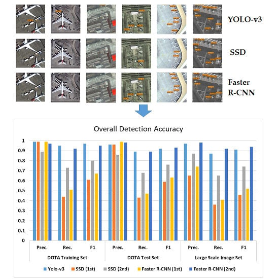
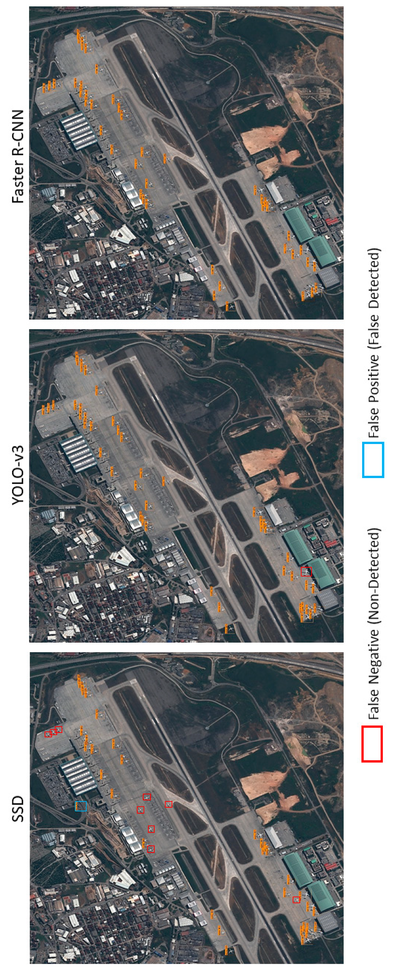
This article presented a comparative evaluation of state-of-the-art CNN-based object detection models for determining airplanes from satellite images. The networks were trained with the DOTA dataset and the performance of them was evaluated with both the DOTA dataset and independent Pleiades satellite images. The best results were obtained with the Faster R-CNN network according to the COCO metrics and F1 scores. The Yolo-v3 architecture also provided promising results with a lower processing time, but SSD could not converge the training data well with low iterations. All of the networks tended to learn more with different parameters and more iterations. It can be asserted that Yolo-v3 has a faster convergence capability when compared with the other networks; however, the optimization methods also play an important role in the process. Although SSD provided the worst detection performance, it was better in object localization. The imbalance between the object sizes and the diversities also affected the results. In the training of deep learning architectures, imbalances should be avoided, or the categories should be divided into finer grains, such as airplanes, gliders, small planes, jet planes, and warplanes. In summary, transfer learning and parameter tuning approaches on pre-trained object detection networks provided promising results for airplane detection from satellite images. Besides, the proposed slide and detect and non-maximum suppression-based detection flow enabled algorithms to be run on full-sized (large-scale) satellite images.

For future work, the anchor box sizes can be defined by weighted clustering according to the sample size of the datasets. Moreover, all of the networks can be used together to define the offsets of the bounding boxes by averaging the predicted bounding boxes, to prevent false positives and increase the recall ratio. In this way, the localization errors could be decreased as well. Finding a way to use the ensemble learning methods for object detection architectures could be another improvement. In addition, the object detection networks often use R, G, and B bands, as they are mostly developed for natural images. However, satellite imageries can contain more spectral bands. Therefore, further studies are planned to integrate the additional spectral bands of the satellite images, to increase the number of labels and train the model more accurately.