A Multi-Observation Least-Squares Inversion for GNSS-Acoustic Seafloor Positioning

Abstract

Monitoring deformation on the seafloor is a major challenge for modern geodesy and a key to better understanding tectonic processes and assess related hazards. The extension of the geodetic networks offshore can be achieved by combining satellite positioning (GNSS) of a surface platform with acoustic ranging to seafloor transponders. This approach is called GNSS-Acoustic (GNSS-A). The scope of this work is to provide a tool to identify and quantify key points in the error budget of such experiment. For this purpose, we present a least-squares inversion method to determine the absolute position of a seafloor transponder array. Assuming the surface platform is accurately positioned by GNSS, the main observables are the two-way travel time in water between the transponders on the seafloor and the surface platform acoustic head. To better constrain transponder positions, we also consider the baseline lengths and the relative depth-differences between different pairs of them. We illustrate the usefulness of our forward modeling approach and least-square inversion by simulating different experimental protocols (i.e., platform trajectories, with or without information on the distance and depth between transponders). We find that the overall accuracy of a GNSS-A experiment is significantly improved with additional information about the relative depths of the instruments. Baseline lengths also improve the accuracy, but only when combined with depth differences. The codes in Python3 used in this article are freely available online.

1. Introduction

Some of the most active tectonic phenomena, among the most devastating, take place on the ocean floor, which covers more than 70 % of the Earth’s surface [1]. For instance, subduction zones generate mega-earthquakes associated with devastating tsunamis (Sumatra in 2004 and Tōhoku–Oki in 2011). In most cases, classic methods of space geodesy (e.g., GNSS) are unable to evaluate the locked or creeping status of faults, because on-land stations are generally too remote from active submarine plate boundaries (subduction and strike-slip faults). Thus, in the past 20 years, new techniques have been developed to extend geodetic observation networks off-shore to fully catch underwater deformation due to tectonic processes. One possibility is to measure the displacement of benchmarks on the seafloor [2].

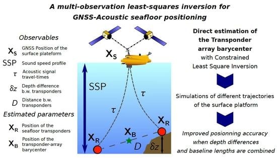
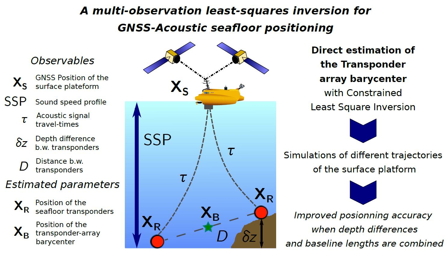
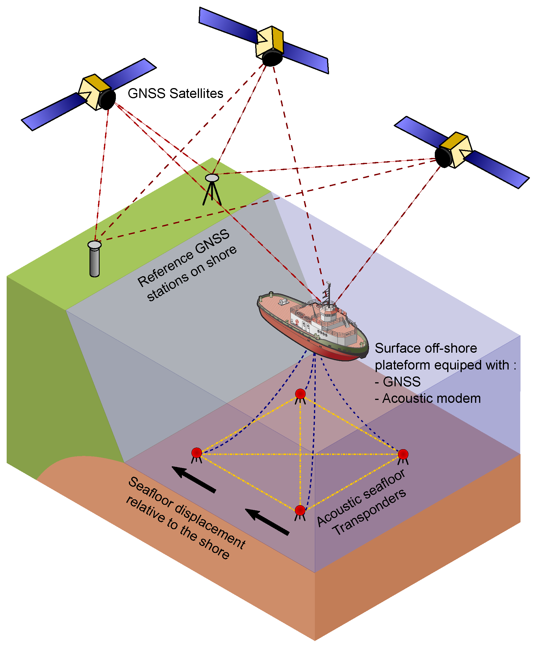
The GNSS-Acoustic (GNSS-A) approach [3] uses a surface platform as a relay between the aerial and underwater media (Figure 1). The position of the platform is obtained in a global reference frame by classical GNSS kinematic processing and is linked by acoustic ranging to a set of transponders permanently installed on the seabed. The displacement and velocity of the submarine benchmarks in a global reference frame can then be derived by repeating these measurements over the years. In this approach, the surface platform comprises GNSS antennas, an acoustic modem to communicate with the transponders on the seafloor, and an inertial system to monitor the motion of the platform (pitch, roll, and heave); all components (antennas and modem) must be referenced to a common origin. Generally, the acoustic head of the modem is chosen as the origin of the platform reference frame, so that its position is precisely known after processing the GNSS data. If we consider the strategy of Spiess et al. [3], the underwater segment has to be an array of several permanent seafloor transponders. The array is considered as a rigid polygon, and its position can be represented by its barycenter (also known as center of figure). Indeed, if measurements are performed at the apex of this point, the errors in the sound-speed profile can be assumed identical for all transponders, thus the horizontal components of the barycenter will remain unaffected. Xu et al. [4] explored a different strategy by accurately positioning a single transponder on the seafloor (single-difference method) or by accurately determining the relative position between two transponders (double-difference method). Combining these approaches over time can then unambiguously measure the absolute displacement of benchmarks on the seafloor and thus deformation of the seafloor. In this paper, we further examine the GNSS-A approach of Spiess et al. [3] by adding constraints such as the baseline lengths or the depth differences between pair of transponders.

The GNSS-A method is mainly used in geophysical applications for monitoring seafloor deformation, which is a key indicator on various processes occurring at depth, such as stress loading on deep faults. Absolute displacement velocities of seafloor benchmarks (in the order of a centimeter to few centimeters/year) is needed to characterize offshore surface deformation due to tectonic processes such subductions. Velocities measured by GNSS-A can then be directly compared to on-shore GNSS observations to estimate deformation gradient between on-shore and off-shore benchmarks and possibly derive the coupling rate of intervening deep faults. This information is crucial to assess the seismic risk. The GNSS-A approach led to notable achievements over the past years, in providing a detailed description of the strain distribution in some subduction zones, for instance, by measuring the co-seismic displacement related to the Tōhoku–Oki earthquake in 2011 (e.g., [5,6]) or by detecting the interplate coupling along segments of the Japan (e.g., [7,8]) or Peru–Chile trenches [9].

Once surface-to-seafloor measurements have been collected over a set of benchmark transponders on the seafloor from a surface platform, the coordinates of the transponders can be restituted by a least-squares (LSQ) inversion [10]. The LSQ method basically consists of adjusting a theoretical model to the observation as closely as possible. However, a multitude of operational models can satisfy this generic definition, depending on the considered observables, the estimated parameters, and how they are related through the so-called observation function.

The three elementary observables for GNSS-A are: (1) the absolute position of the acoustic modem in an external reference frame; (2) some water sound-speed information; and (3) the two-way travel (TWT) times between the acoustic modem and the seafloor transponders. The elementary estimated parameters are the transponder positions. However, it is also possible to adjust some other parameters. For instance, Fujita et al. [11] proposed an iterative approach in two steps: a determination of the transponder positions, and then a polynomial adjustment of the sound-speed profile. Ikuta et al. [12] described a method allowing a correction estimation of the tie vector between the acoustic modem and the GNSS antenna positions on the ship. Xu et al. [4] considered the differences between two consecutive rangings to eliminate long-term changes in the sound-velocity.

Additional observables constraining the geometry of the transponder array can also be integrated into the model to improve the positioning precision. The depths and relative positions of the transponders can be assessed by towing an acoustic interrogator a few dozen meters above the seafloor transponders [10,13]. Their depth can also be measured by pressure sensors [9,14,15,16,17]. The geometry of the array can also be determined from a preliminary survey of each transponder from a surface vessel [4,18,19]. In addition, baseline lengths between pairs of transponders can be directly measured in adequate configuration by acoustic ranging, and, instead of absolute depths, relative depth differences between each transponder can also be considered.

One of the aims of this study was to provide a tool to help identify and quantify the error budget of a GNSS-A experiment. For this purpose, we explicate and detail a LSQ model to perform a GNSS-Acoustics positioning, taking as main inputs the acoustic TWT times and the positions of the platform, with additional observations mentioned above. We also describe a way to directly estimate the array barycenter coordinates. We illustrated the possibilities of the model through simple but realistic simulations. We quantified the effects of the different combinations of additional observations on the accuracy of the seafloor positioning. Finally, we examined the influence of the platform trajectory during a GNSS-A experiment on the error budget (i.e., if the platform does not hold a station above the barycenter of the transponder array).

2. Seafloor Coordinates Restitution Model

2.1. Least-Squares Approaches

Least-squares methods are commonly used in geodesy (e.g., [20]). They allow adjusting parameters of a known model to a dataset and find the parameters that best fit the data (i.e., for which the sum of the square of the residues is minimum). They have the advantage of being linear, which eases their implementation and helps run a large number of simulations and tests. LSQ approaches are widely documented in the literature and can be described in many different ways. Here, we present a general formulation adapted to our problem and show how to combine observations or observable quantities (input data) of different types and to constrain them to certain values to obtain estimates of unknown parameters (output data). The notation conventions are given in the Supplementary Materials (Section S1).

2.2. Estimated Output Parameters

The objective of a GNSS-A experiment is to precisely position an array of seafloor transponders, considered as benchmarks, or the whole array as a single benchmark. The relative positions of the transponders are assumed as fixed, and no movement affects the array during a measurement campaign. If we have $n_R$ transponders, the position of ith transponder $R_i$ ($i\in 〚1,n_R〛$) is denoted ${\mathbf{X}}_{R_i}=[x_{R_i},y_{R_i},z_{R_i}]$.

The strategy of Spiess et al. [3] is to consider the seafloor transponder array as a rigid polygon, and then estimate the displacement of the whole array, instead of that of each instrument. Thus, the array barycenter can represent the complete array position. Then, we focus our method on the determination of the barycenter coordinates. We note ${\mathbf{X}}_G=[x_G,y_G,z_G]$ the coordinates of the barycenter.

We have, by definition:

$${\mathbf{X}}_G=\sum _{i=1}^n{\displaystyle \frac{{\mathbf{X}}_{R_i}}{n_R}}$$

(1)

The purpose of our data inversion is to find the coordinates ${\mathbf{X}}_{R_i}$ and/or ${\mathbf{X}}_G$.

2.3. Input Data (Observations)

To solve ${\mathbf{X}}_{R_i}$ and/or ${\mathbf{X}}_G$, it is necessary to have at minimum the following observations:

• A sound-speed profile (SSP), represented as two vectors $\mathbf{Z}$, $\mathbf{C}$, corresponding to depths and associated sound-speeds.
• The position of the surface acoustic head ${\mathbf{X}}_S=[x_S,y_S,z_S]$ in a local topocentric reference frame i.e., an east, north, up reference frame, with an arbitrary point of the working area taken as the origin.
• Two-way travel times of acoustic pings $\tau$ between the surface acoustic head and the seafloor acoustic devices.

Additional information can improve positioning:

• The depth of the transponders, measured either with pressure sensors embedded in the transponders [9,15] or a probe [13]. However, instead of considering absolute depths, since pressure sensors can be ill-calibrated and water density profiles are hard to assess (e.g., [21]), we design a least-squares model to handle relative depth differences $\delta z$ between pairs of instruments.
• The distance between pairs of transponders, hereinafter termed baseline length. Measuring in situ the array geometry provides an important constraint to determine the transponder coordinates [10]. This can be achieved during a preliminary acoustic survey from the surface [16,18] or by towing a vehicle [13]. Alternatively, transponders can directly communicate with one another when the baseline length is short enough. Distances are then derived from the two-way travel times of an acoustic signal between two devices and from the sound-speed [22,23].

The acoustic head position is time dependent due to the constant motion of the platform on the sea-surface (displacement and sea-state). Thus, considering a measurement campaign during a period T starting at $t_0$, at every time $t\in \left[t_0,t_0+T\right]$, the surface modem position is a function of t: ${\mathbf{X}}_S\left(t\right)=[x_S\left(t\right),y_S\left(t\right),z_S\left(t\right)]$. Two-way travel times also depend on t. If a measurement campaign comprises $n_{\tau }$ pings, we will have $n_{\tau }\times n_R$ round-trip time ${\tau }_{i,R_j}\left(t\right)$ with $i\in 〚1,n_{\tau }〛$ and $j\in 〚1,n_R〛$.

2.4. Two-Way Travel Times: Observation Function and Associated Design Matrix

The observation function $f_{SMA}$ (SMA for SubMarine Acoustics) is here an eigenray research function, as described, for instance, by Sakic et al. [24]. It provides propagation time $\tau$ of the eigenray between the emitter ${\mathbf{X}}_S$ and receiver ${\mathbf{X}}_R$ for a given SSP $\mathbf{C}$. Since we are only searching for ${\mathbf{X}}_R$, this is the only variable that f takes as an unknown parameter. The other input observations ${\mathbf{X}}_S$ and $\mathbf{C}$ are not considered as observables in the least squares sense (they are not appended to vector $\mathbf{L}$ as defined in the Supplementary Materials). However, they change over time, thus are treated as constant for a given epoch, but vary from one epoch to another. The different $\mathbf{C}$ for each epoch can be determined for instance by interpolating two successive Conductivity/Temperature/Depth (CTD) profiles to account for the temporal variation of the SSP, which is the main source of error in a GNSS-A experiment (e.g., [10,25]). Similarly, ${\mathbf{X}}_S$ can also be interpolated for each epoch from the platform discrete GNSS trajectory. We call these “epoch-dependant constants” $\mathsf{\Omega }$, and we have ${\mathsf{\Omega }}_{SMA}=[{\mathbf{X}}_S,\mathbf{C}]$.

$$\begin{array}{c}\hfill f_{SMA}:\left({\mathbf{X}}_R,{\mathsf{\Omega }}_{SMA}\right)⟼\tau \end{array}$$

(2)

The observation function provides theoretical values of the propagation times ${\tau }_{theo}$ to the receiver a priori positions ${\mathbf{X}}_R$.

Snell–Descartes ray-tracing as an observation function for the least-squares inversion provides the best compromise in terms of accuracy and computation time [24]. Since our scope is mainly to analyze observable effects, lateral heterogeneities in the ocean will not be considered here.

If $n_R$ transponders are used, the associated design matrix ${\mathbf{A}}_{SMA}$ is block-diagonal and of size $(n_{\tau }·n_R,3n_R)$, in the ideal case where each transponder has responded to $n_{\tau }$ pings send from the surface.

Displacement of the Surface Platform during Ping Propagation

For an experiment in deep waters (5000 m), the order of magnitude of a TWT time is ∼7 s. During this time, the surface platform is likely to move because of the sea-state (swell and waves), even if it is trying to hold a fixed position. If neglected, a typical displacement in the order of 1 m may introduce an error in the transponder positions.

To account for the displacement of the platform between the ping emission and reception and to solve what we call the forward/backward problem, we redefine the observation function $f_{SMA}$ as follows: We assume that the positions of the platform when the ping is emitted and received, respectively ${\mathbf{X}}_{S,emi}$ and ${\mathbf{X}}_{S,rec}$, are known. We search independently the characteristics of the eigenrays corresponding to the emission phase $\left({\tau }_{emi}\right)$ and to the reception phase $\left({\tau }_{rec}\right)$. The total propagation time ${\tau }_{F/B}$ is the sum of both. Then, the new observation function $f_{SMA,F/B}$ becomes:

$$\begin{array}{}\mathrm{(3)}& \hfill {\tau }_{F/B}& ={\tau }_{emi}+{\tau }_{rec}\hfill \mathrm{(4)}& \hfill & =f_{SMA}({\mathbf{X}}_R,{\left[{\mathbf{X}}_{S,emi}\right]}_{\mathsf{\Omega }})+f_{SMA}({\mathbf{X}}_R,{\left[{\mathbf{X}}_{S,rec}\right]}_{\mathsf{\Omega }})\hfill \mathrm{(5)}& \hfill & =f_{SMA,F/B}({\mathbf{X}}_R,{\left[{\mathbf{X}}_{S,emi},{\mathbf{X}}_{S,rec}\right]}_{\mathsf{\Omega }})\hfill \end{array}$$

In terms of computation, the forward/backward mode, therefore, doubles the number of ray tracing operations.

2.5. Direct Estimation of the Barycentrer Coordinates

As mentioned in Section 2.2, we want to determine the barycenter coordinates of the polygon shaped by several transponders. There are two ways to estimate ${\mathbf{X}}_G$. The most intuitive one consists in determining the individual position of each transponder, and then to derive the position of the barycenter as in Equation (1). The second method consists in directly determining the barycenter coordinates ${\mathbf{X}}_G=[x_G,y_G,z_G]$ in the LSQ inversion. Since the barycenter is immaterial, its coordinates cannot be derived from direct observations. Instead, we use the coordinate differences $\Delta x,\Delta y,\Delta z$ between a transponder position and the barycenter: ${\mathbf{X}}_R=[x_G+\Delta x_R,y_G+\Delta y_R,z_G+\Delta z_R]={\mathbf{X}}_G+\Delta {\mathbf{X}}_R$.

Since:

$$\begin{array}{}\mathrm{(6)}& \hfill {\mathbf{X}}_G& =\sum _{i=1}^{n_R}{\displaystyle \frac{{\mathbf{X}}_{R_i}}{n_R}}\hfill \mathrm{(7)}& \hfill & =\sum _{i=1}^{n_R}{\displaystyle \frac{{\mathbf{X}}_G+\Delta {\mathbf{X}}_{R_i}}{n_R}}\hfill \mathrm{(8)}& \hfill & ={\mathbf{X}}_G+\sum _{i=1}^{n_R}{\displaystyle \frac{\Delta {\mathbf{X}}_{R_i}}{n_R}}\hfill \end{array}$$

it follows that:

$$\sum _{i=1}^{n_R}\Delta {\mathbf{X}}_{R_i}=0$$

(9)

Therefore, searching for the barycenter position imposes the additional constraint that the sum of the differences of coordinates must be equal to zero. This approach increases the number of unknowns to $3n_R+3$. The vector of unknowns becomes:

$$\mathbf{X}={\left[\begin{array}{ccccccc}{x}_G,& y_G,& y_G,& \Delta x_{R_1},& \Delta y_{R_1},& \Delta z_{R_1},& \cdots \end{array}\begin{array}{ccc}\Delta x_{R_n},& \Delta y_{R_n},& \Delta z_{R_n}\end{array}\right]}^{⊺}$$

(10)

Because ${\mathbf{X}}_R={\mathbf{X}}_G+\Delta {\mathbf{X}}_R$, we have the following relation to constitute the design matrix:

$$\frac{\mathrm{d}{f}_{SMA,\tau }}{\mathrm{d}{\mathbf{X}}_R}=\frac{\mathrm{d}{f}_{SMA,\tau }}{\mathrm{d}{\mathbf{X}}_G}=\frac{\mathrm{d}{f}_{SMA,\tau }}{\mathrm{d}\Delta {\mathbf{X}}_R}$$

(11)

The design matrix details and the associated Helmert constraint sub-matrices are described in the Supplementary Materials (Section S4).

3. Geometry Constraints: Baseline Lengths and Depth Observations

3.1. Baseline Length Observations

In this approach, we suppose that the geometry of the transponder array could be given by baseline lengths, directly measured between each pair of transponders. We note $D_{AB}$ the Euclidean distance between two transponders $R_A$ and $R_B$ of coordinates ${\mathbf{X}}_{R_A}=\left[x_{R_A},y_{R_A},z_{R_A}\right]$ and ${\mathbf{X}}_{R_B}=\left[x_{R_B},y_{R_B},z_{R_B}\right]$.

We have, by definition:

$$\begin{array}{cc}\hfill D_{AB}& =\parallel {\mathbf{X}}_{R_B}-{\mathbf{X}}_{R_A}\parallel \hfill \\ \hfill & =\sqrt{{(x_{R_B}-x_{R_A})}^2+{(y_{R_B}-y_{R_A})}^2+{(z_{R_B}-z_{R_A})}^2}\hfill \end{array}$$

(12)

If we have $n_R$ transponders, we can add the baseline lengths as observations $L_{i,j}$ with $i,j\in 〚1,n_R〛$. We call $n_D$ the number of baselines theoretically observables. We have $n_D=n_R+\frac{n_R(n_R-3)}{2}$ (if all baselines are measured). The relation in Equation (12) constitutes an observation function which at the coordinates of two transponders associates the length of the corresponding baseline.

We have:

$$f_D({\mathbf{X}}_{R_A},{\mathbf{X}}_{R_B})⟼D_{AB}$$

(13)

This function can be easily derived analytically. The design matrix and associated vector enhancements are described in the Supplementary Materials (Section S3).

3.2. Estimation of a Single Depth

If we assume as a first approximation that all the transponders are at the same depth z, e.g., are laying on a flat abyssal plain, we can search for the unknown depth component noted $\overline{z}$. It can be either the depth of a transponder arbitrary considered as a reference or the barycenter depth $z_G$. This case reduces the number of unknowns from $3n_R$ to $2n_R+1$. The least-squares model implementation is described in the Supplementary Materials (Section S5).

3.3. Adjusting Depths with Relative Observations

Tectonically active areas often display a rough seafloor and a single $\overline{z}$ hypothesis may not be realistic in most experiments. Precise deployments and accurate mapping of the bathymetry, or post-deployment acoustic ranging may provide the actual depth of each transponder. However, due to uncertainties in sound-speed profiles, the acoustic transponder depths are generally only correct relative to each other. Similarly, due to calibration uncertainties, deep-sea pressure sensors may not provide correct depth values but correct depth differences among sensors. To take advantage of this “more accurate” information, a solution is to introduce the additional input observations $\delta z=z_{R_i}-\overline{z}$, linking each transponder to an unknown reference depth. These $\delta z$ can then be considered as observables in the least-squares sense or as known constant data.

3.3.1. Depth Differences as Observables in the Least-Squares Sense

Considering depth-differences as observables in the least-squares sense is only pertinent when the barycenter is directly estimated, as described in Section 2.5. The vector of unknowns $\mathbf{X}$ is described in Equation (10). If we have a depth-difference observation $\delta z_{AB}$ between two transponders $R_A$ and $R_B$ such that $\delta z_{AB}=z_{R_B}-z_{R_A}=\Delta z_{R_B}-\Delta z_{R_A}$, where $\Delta z$ are the eccentricities with respect to the barycentrer introduced in Section 2.5, then we have a new observation function:

$$f_z:(z_{R_A},z_{R_B})⟼\delta z_{A,B}$$

(14)

The design matrix and associated vector enhancements are described in the Supplementary Materials (Section S6).

3.3.2. Constant Depth Differences

Considering depth-differences $\delta z_{R_i}$ as constants works only if we estimate a single depth $\overline{z}$ for all transponders. We can, however, use the ray tracing function to find the eigenray for each transponder between the emission point ${\mathbf{X}}_S$ and the seafloor point ${\mathbf{X}}_{R_i}=[x_{R_i},y_{R_i},\overline{z}+\delta z_{R_i}]$.

3.3.3. Differences between Both Approaches

There is a difference between the two approaches described above. In the first one, depth differences are considered as observables in the least-squares sense, thus we can assign them weights, and get fitting residuals after the inversion. In the second one, depth differences are used as simple “inert” constants. Choosing one approach or the other mainly depends on the reliability of these observations. The second is the simplest, but a likely source of error: imprecise $\delta z$ will have a direct effect on $\overline{z}$ estimation, because no weighting is possible.

4. Testing the Least-Squares Inversions with Different Observation Types

We simulated several experiments with different type of observations in order to evaluate their contribution and determine optimal combinations of observations. We considered a square-shaped array. In such geometry, the distances (or acoustic rays) between each transponder and the surface modem above the square barycenter are all equal, thus temporal changes in the sound-speed profile during the experiment should not affect the horizontal positioning of the barycenter. Moreover, it is the simplest configuration for deploying four transponders, which also provides some redundancies relative to a triangle-shaped array. 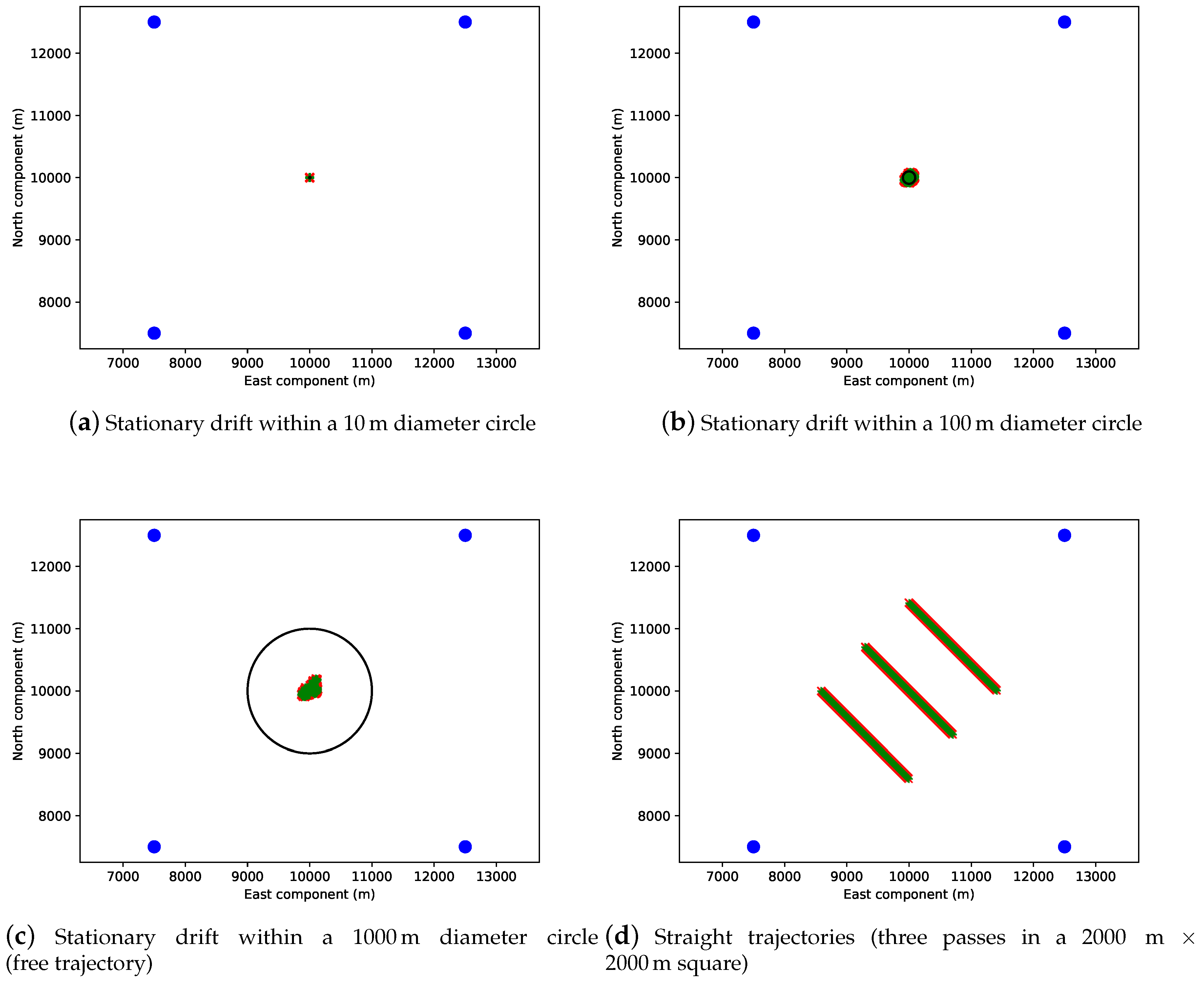However, more complex geometries were tested by Kido [26]. We simulated four different surface-platform trajectories centered above the barycenter of the transponder array, to reproduce a complete GNSS-A experiment, as described by Spiess et al. [3]. The different trajectories are represented in Figure 2. The first three are “drifting” trajectories and implemented as random walks:

• a trajectory inscribed in a 10 m radius circle (short-named R10);
• a trajectory inscribed in a 100 m radius circle (short-named R100);
• a trajectory inscribed in a 1000 m radius circle (short-named R1000) (in this case, however, the implemented random walk never reaches the circle limit, and thus can be considered as a free trajectory); and
• a series of three straight and parallel profiles inscribed in a square of 2000 m × 2000 m (short-named 3×333).

The other parameters were the same in the four experiments:

• The four transponders on the sea-bottom were “deployed” at the corners of a square of 5000 m a side, at a depth of 5000 m. The depths of the transponders were shifted by, respectively, +10, $-20$, +30, and $-40$ m to represent the non-planarity of the ocean floor. Thus, the depths of the transponders were, respectively, 5010, 4980, 5030, and 4960 m.
• Their positions were then modified with a metric error. These noised positions were used as initial a priori estimates in the least-squares inversion. They represented the approximate positions obtained during a preliminary survey of each transponder, which is a fundamental first step in a GNSS-A experiment to determine the array internal geometry [3,14,27].
• The surface-platform trajectory was noised with a white noise of standard deviation ${\sigma }_{xy}=2$ cm in the horizontal components and ${\sigma }_z=5$ cm in the vertical component, aiming at representing current precision in absolute kinematic GNSS positioning (e.g., [28]). The straight-line trajectories remained a theoretical example designed for the simulations, since following a perfectly linear trajectory is hardly achievable for a ship.
• We “acquired” 1000 acoustic pings along each trajectory (333 per pass for the straight tracks).
• The acoustic observations $\tau$ were noised to represent the random behavior of the ocean. The perturbation was based on an empirical analysis of oceanographic measurements performed by moored buoys from the Caribbean MOVE network [29]. Probes along moorings provided sound velocities as a function of time at several depths. It led to a resulting perturbation in the order of 10⁻⁴ s. 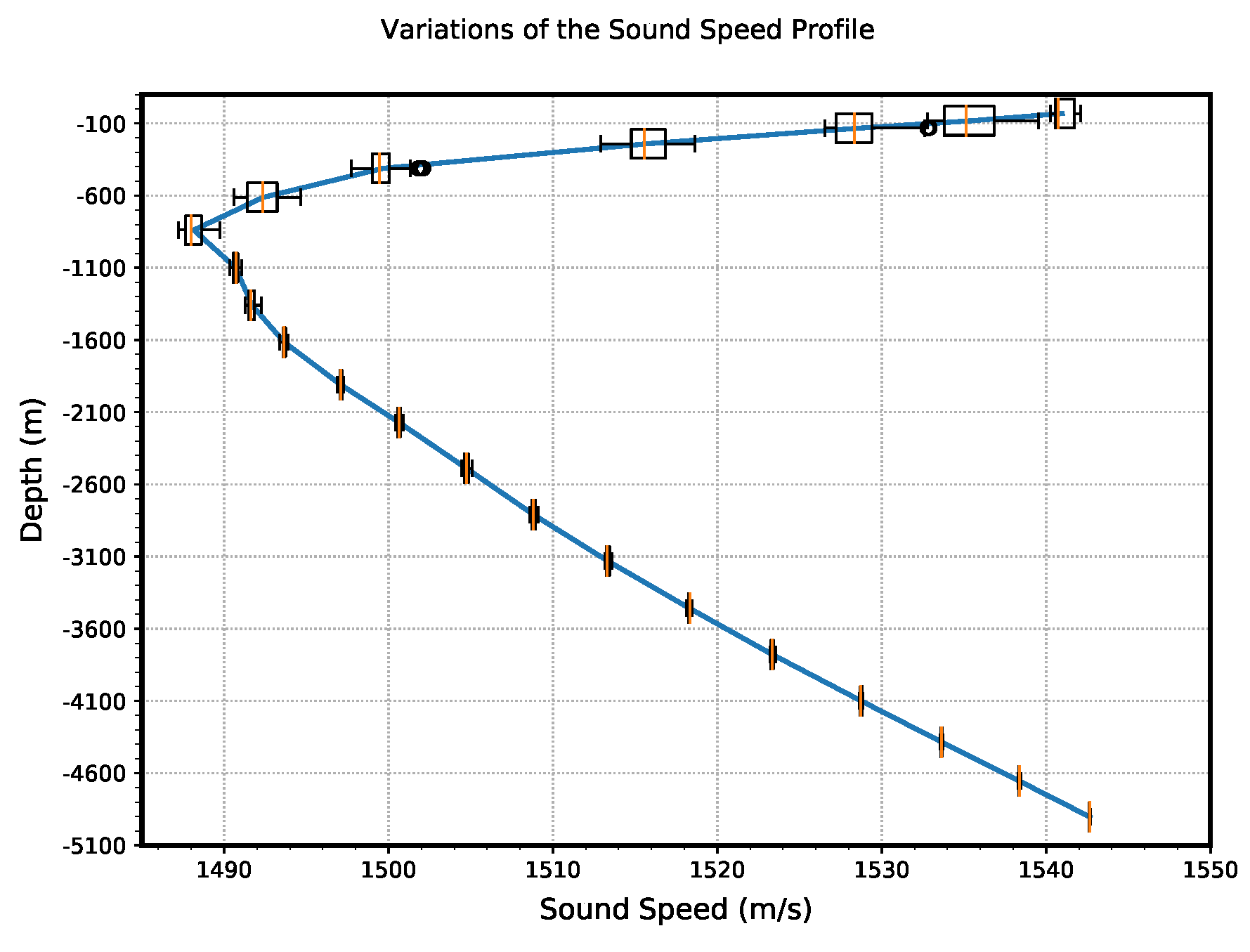For a nominal propagation time of around $3.5$ $\mathrm{s}$, this value can be considered as pessimistic. Nevertheless, it remained relevant for a theoretical relative comparison of the different inversion schemes. The standard SSP used in the simulations, along with the applied perturbations, is represented in Figure 3.
• A random hardware uncertainty of ${\varsigma }_{hw}={10}^{-5}$ s corresponding to the signal detection error, was added to the TWT times $\tau$, according to state-of-the-art material specifications (e.g., [30]).
• The baseline lengths were noised with a millimeter error, commonly observed in recent seafloor acoustic ranging experiments [31,32,33]. The influence of the depth-difference precision was also tested (see Section 5).
• For estimating the barycenter coordinates in the least-squares inversion, we used a single velocity profile, as the one used for generating the observations (blue curve in Figure 3, without noise).
• Finally, acoustic observations, baseline lengths, and depth differences were, respectively, weighted with standard deviation values ${\varsigma }_{SMA}={10}^{-5}$ s, ${\varsigma }_D={10}^{-3}$ m, and ${\varsigma }_z={10}^{-2}$ m.

The difference between the true position of the barycenter of the transponder array (known here because data were artificially generated) and the position of the barycenter restituted by the LSQ was used as the main quality indicator.

Since horizontal seafloor motion monitoring was our final goal, we only considered the planimetric distance difference involving the x and y components of the barycenter position (i.e., 2D differences).

We call this difference $E_{G,2D}$:

$$E_{G,2D}=\sqrt{{({\widehat{x}}_G-{\dot{x}}_G)}^2+{({\widehat{y}}_G-{\dot{y}}_G)}^2}$$

(15)

with ${\widehat{\mathbf{X}}}_G=[{\widehat{x}}_G,{\widehat{y}}_G,{\widehat{z}}_G]$ the estimated barycenter coordinates and ${\dot{\mathbf{X}}}_G=[{\dot{x}}_G,{\dot{y}}_G,{\dot{z}}_G]$ the true barycenter coordinates.

Note that the mode where $\delta z$ were used as observations was only implemented in combination with baseline lengths observations and direct barycenter estimation.

4.1. Results

Results for the different experimental settings are shown in Figure 4 and

Table 1. Distance to true barycenter for different inversion protocols for a drifting trajectory inscribed in a 10 m radius circle.

		Barycentrer Direct Estimation	With Baselines	Single Depth Estimation $\overline{\mathit{z}}$	With $\mathit{\delta }\mathit{z}$ as Constants	With $\mathit{\delta }\mathit{z}$ as Observations	${\mathit{E}}_{\mathit{G},2\mathit{D}}$ (m)
A1	▴	–	✓	✓	✓	–	0.000697971
A2	▴	✓	✓	✓	✓	–	0.000698204
B1	▴	✓	✓	–	–	✓	0.00196695
C1	▴	–	–	✓	✓	–	0.460023
C2	▴	✓	–	✓	✓	–	0.466254
D1	▴	✓	✓	–	–	–	0.862794
D2	▴	–	–	–	–	–	0.870165
D3	▴	–	✓	–	–	–	0.878651
D4	▴	✓	–	–	–	–	0.879655
E1	▴	–	–	✓	–	–	26.1199
E2	▴	✓	–	✓	–	–	26.1256

,

Table 2. Distance to true barycenter for different inversion protocols for a drifting trajectory inscribed in a 100 m radius circle.

		Barycentrer Direct Estimation	With Baselines	Single Depth Estimation $\overline{\mathit{z}}$	With $\mathit{\delta }\mathit{z}$ as Constants	With $\mathit{\delta }\mathit{z}$ as Observations	${\mathit{E}}_{\mathit{G},2\mathit{D}}$ (m)
A1	▴	–	✓	✓	✓	–	0.000684927
A2	▴	✓	✓	✓	✓	–	0.000685106
B1	▴	✓	✓	–	–	✓	0.0073727
C1	▴	–	–	✓	✓	–	0.0236024
C2	▴	✓	–	✓	✓	–	0.0236294
D1	▴	✓	–	–	–	–	0.0478391
D2	▴	–	✓	–	–	–	0.0478509
D3	▴	–	–	–	–	–	0.0478525
D4	▴	✓	✓	–	–	–	0.0478672
E1	▴	✓	–	✓	–	–	23.3008
E2	▴	–	–	✓	–	–	23.301

,

Table 3. Distance to true barycenter for different inversion protocols for a drifting trajectory inscribed in a 1000 m radius circle.

		Barycentrer Direct Estimation	With Baselines	Single Depth Estimation $\overline{\mathit{z}}$	With $\mathit{\delta }\mathit{z}$ as Constants	With $\mathit{\delta }\mathit{z}$ as Observations	${\mathit{E}}_{\mathit{G},2\mathit{D}}$ (m)
A1	▴	–	✓	✓	✓	–	0.000696966
A2	▴	✓	✓	✓	✓	–	0.000697191
B1	▴	✓	✓	–	–	✓	0.00609881
C1	▴	✓	–	✓	✓	–	0.0101206
C2	▴	–	–	✓	✓	–	0.0101255
D1	▴	✓	–	–	–	–	0.0225603
D2	▴	–	–	–	–	–	0.022636
D3	▴	–	✓	–	–	–	0.0230085
D4	▴	✓	✓	–	–	–	0.0230226
E1	▴	✓	–	✓	–	–	23.024
E2	▴	–	–	✓	–	–	23.0245

and

Table 4. Distance to true barycenter for different inversion protocols for a three straight lines trajectory.

		Barycentrer Direct Estimation	With Baselines	Single Depth Estimation $\overline{\mathit{z}}$	With $\mathit{\delta }\mathit{z}$ as Constants	With $\mathit{\delta }\mathit{z}$ as Observations	${\mathit{E}}_{\mathit{G},2\mathit{D}}$ (m)
A1	▴	–	✓	✓	✓	–	0.00156857
A2	▴	✓	✓	✓	✓	–	0.00156869
C1	▴	✓	–	✓	✓	–	0.00339649
C2	▴	–	–	✓	✓	–	0.00339676
B1	▴	✓	✓	–	–	✓	0.00611405
D1	▴	✓	–	–	–	–	0.00620074
D2	▴	–	–	–	–	–	0.00620086
D3	▴	✓	✓	–	–	–	0.00621065
D4	▴	–	✓	–	–	–	0.00621092
E1	▴	–	–	✓	–	–	25.7488
E2	▴	✓	–	✓	–	–	25.8065

. The different inversion modes are sorted from best to worst based on the barycenter indicator $E_{G,2D}$ (i.e., 2D distance to true barycenter). They are arranged in five groups, separated in the tables by horizontal bars.

Inversion imposing a single depth for all the transponders (Modes Ex) turns out to be irrelevant: $E_{G,2D}$ reaches an order of several tens of meters. Inversion modes with TWT times only but without additional depth observations (Modes Dx) can be considered as relevant, but are unstable and highly dependant on the surface trajectory. The accuracy level varies from millimeters for a straight trajectory to decimeters for trajectories inscribed in a small circle.

4.1.1. Optimal Strategies

Two main inversion strategies emerge: one with a single depth estimation with the addition of the $\delta z$ as constants (Modes Ax and Cx) and the other with direct barycenter estimation with the addition of $\delta z$ as observables in the least-squares sense (Mode B1). The modes using $\delta z$ as constants are improved when baseline lengths are taken into account in the inversion (Modes Ax). The accuracy level varies from centimeters (decimeters for trajectories inscribed in a small circle) to sub-millimeters (millimeters for straight trajectories) when baseline lengths are considered. For the mode using $\delta z$ as observables in the least-squares sense (B1), the accuracy is millimetric and stable for all trajectories.

Thus, additional depth observations improve the accuracy by one order of magnitude compared to an equivalent mode without depth-difference observations. Moreover, baseline lengths contribute to improve the final position of the barycenter, but only if depth differences are jointly used. Thus, baseline lengths are less influential than depth-difference observations. We also confirm that, whatever the processing mode, directly estimating the barycenter or not produces the same results. It is an expected behavior, but it validates a direct barycenter estimation as a pertinent conceptual improvement, since formal standard deviations related to its coordinates can be directly determined.

4.1.2. Trajectory Influence

Trajectories of the surface platform have a strong influence on the restitution accuracy. With a trajectory inscribed in a 10 m circle, the parameter $E_{G,2D}$ reaches almost 90 cm, contrasting with centimetric values when the inscribed circle is bigger. This can be explained by the geometrical weakness of the trajectory shape in a simulation context where lateral sound-speed heterogeneities do not contribute: a redundancy of similar observations does not improve the solution.

When no depth observations are used, a straight trajectory provides better results (about one order of magnitude) than the circle-inscribed trajectories. This is due to a simulation artifact, because the trajectory is perfectly symmetrical with respect to the transponder array and therefore the errors are compensated.

5. Influence of the Precision in the Depth-Difference Measurements

Since the depth-difference parameter is the most important, and since for some of the inversion modes the parameter $\delta z$ will be constant and not adjustable, we tested the influence of $\delta z$ uncertainties on the indicator $E_{G,2D}$. We considered the Modes A2 ($\delta z$ fixed) and B1 ($\delta z$ as observables in the least-squares sense) and the four trajectories defined above. The quality of $\delta z$ was progressively degraded from a millimetric to a metric uncertainty: we added to depth-difference observations a Gaussian random value ranging between 10⁻³ m and 1 $\mathrm{m}$. 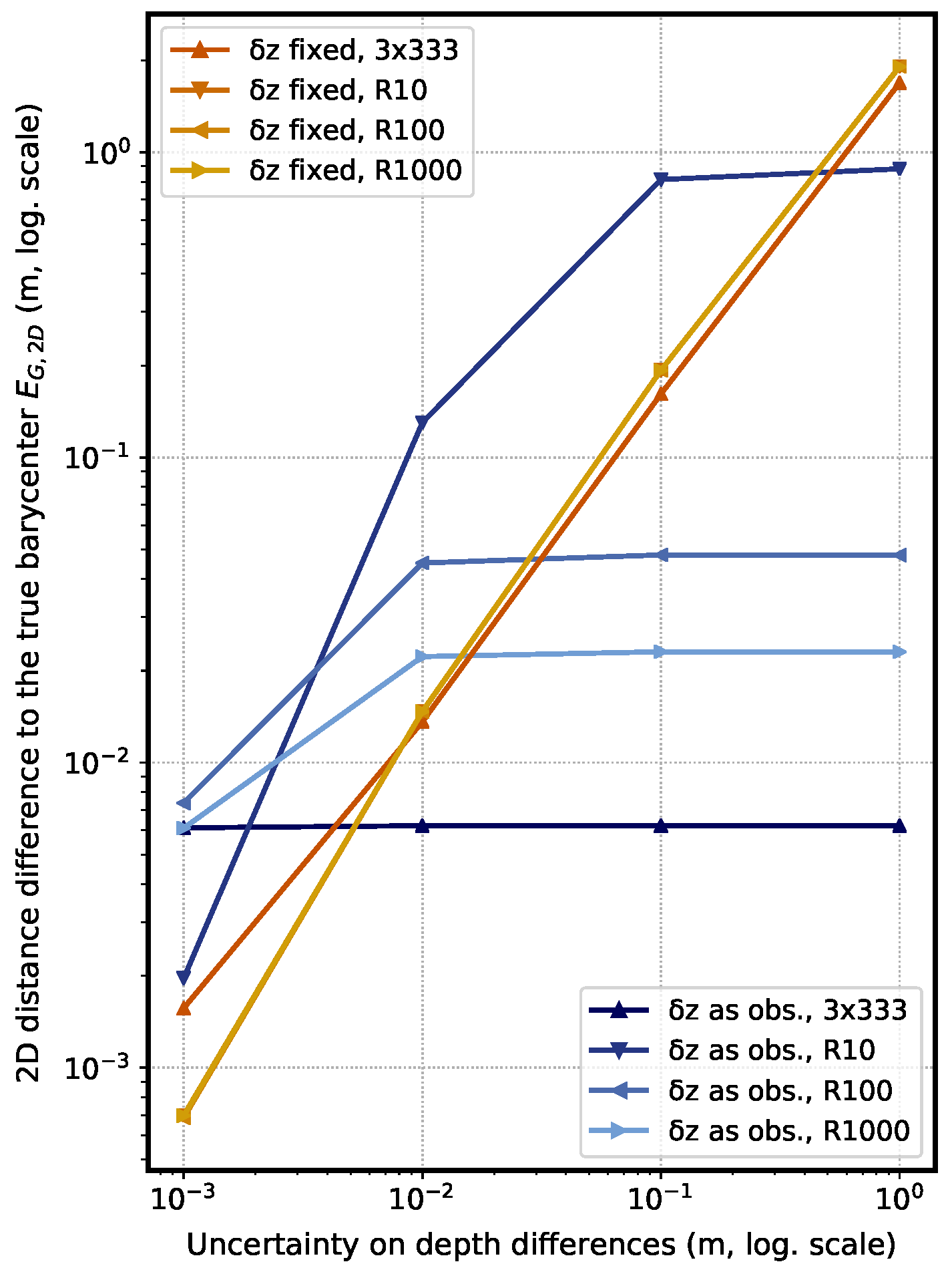The results are presented in Figure 5.

The influence of the $\delta z$ precision for “fixed” cases (warm colors) is clear. The coarser the depth-difference precision is, the worse the restituted barycenter position accuracy becomes. The accuracy degradation is in the same order of magnitude as the $\delta z$ precision level, regardless of the trajectory. The behavior is different when $\delta z$ are used as observables in the least-squares sense (cold colors) and $E_{G,2D}$ values depend on the trajectory. Better values are obtained for straight trajectories (Figure 4d) than for inscribed circle trajectories (Figure 4a–c), and, for the latter, the values worsen as the diameter of the circle gets bigger. We also notice that for trajectories over a 100 m span and for $\delta z$ over a centimeter precision level, there is no more influence of the depth-difference information on $E_{G,2D}$. For a trajectory inscribed in a 10 m circle, $E_{G,2D}$ improves as the $\delta z$ precision improves. Nevertheless, for our geophysical applications which are aiming at a centimetric level, there is a real benefit only when the depth-difference precision is below a centimeter level. Note that today, such an accuracy level is difficult to achieve for the considered depth ranges (several thousand meters), as it is a function of the water-depth.

6. Influence of the Forward/Backward Mode

To test the influence of the forward/backward mode (Section 2.4), which takes into account the movement of the platform between a ping emission and its reception, we considered the restitution Mode B with baseline length and $\delta z$ as observables in the least-squares sense.

Table 5. Distance to true barycenter with an inversion with or without forward/backward mode for the four simulated trajectories considered, using an inversion mode with baseline lengths and $\delta z$ as observables.

(mm)	With F./B. Mode	Without F./B. Mode	Difference
R10	1.96	08.87	6.90
R100	7.37	10.04	2.67
R1000	6.09	12.81	6.71
3×333	6.11	4636.54	4630.43

compares the results for the four trajectories whether the platform position is considered the same at the emission and reception instants or different (forward/back-ward mode).

Implementing the forward/backward mode improves the accuracy of the barycenter position by several millimeters for all trajectories inscribed in a circle. It even corrects an important instability of several meters for the straight trajectories. This instability can be explained by the exact symmetry of the platform trajectory relative to the barycenter, which produces repeated observations with the same values. This is a simulation artifact, which, of course, cannot be reproduced in a real experiment.

7. Discussion

As typical plate velocities are in the order of a centimeter or few centimeters per year, most geophysical applications require at least a centimeter precision level for a seafloor positioning. In the GNSS-A method, the main inputs are the TWT times between the seafloor transponders and the surface modem. We have shown that the positioning solution can be significantly improved by adding ancillary observations.

7.1. Depth Observations

As shown in Section 4.1, using depth-difference information (Modes Ax, B1, and Cx) gives the best results, leading to a centimetric accuracy. The mode using depth difference (B1) as observables in the least-squares sense is preferred mainly because it is possible to assign a weight to the observable $\delta z$ depending on its quality. Fixed depth differences (Ax and Cx) can be useful, but should only be considered if their precision level is better than a centimeter, as shown in Section 5. In any case, it is better to take advantage of a height difference information in the inversion.

Simulations without depth-difference information (Mode Dx) lead to degraded results, exceeding the centimeter accuracy level (close to a meter level for the trajectory in a 10 m radius circle). This is likely due to the noising strategy that overestimates the noise in the acoustic ranging values.

The recent advent of self-calibrating pressure sensors [34,35] is very promising for GNSS-A experiments. First, they can improve the accuracy of the transponder depths or depth-differences, which are shown to significantly improve the solution. Second, a drift-controlled sensor will reduce the uncertainties in the sound-speed inferred from pressure, temperature and conductivity sensors.

7.2. Baseline Length Observations

Information on the baseline lengths also improves the final accuracy, but only when combined with depth differences (Modes Ax and B1). We considered a millimeter perturbation added to baseline lengths based on recent acoustic-ranging experiments [31,33], but we are aware that it might be optimistic given the size of our array (5 km × 5 km square) compared to these experiments. Moreover, with state-of-the-art transponders, a millimeter precision level is only achieved in relative variation detection. Indeed, even though TWT times can be measured with a nano-second accuracy, the accuracy in the distance determination is highly dependent on the accuracy in the sound-speed. Sound-speed sensors, or conductivity/temperature/pressure sensors are often not accurate enough or subject to long-term drifts. This difficulty warrants further studies on direct ranging processing methods [32]. Our study aimed at evaluating the advantage of knowing the baseline lengths, but not at giving practical experimental procedures that are dependant on local configuration and available instrumentation evolving with time.

For acquiring baseline data, the inter-visibility between transponders must be carefully considered, because submarine reliefs and ray bending can prevent direct acoustic communications. A preliminary bathymetric survey will help to detect potential obstacles, and to select the appropriate sites for the transponders. The transponder supporting frames must also be carefully designed: they must be stable and high enough both to ensure an optimal inter-visibility and to minimize multi-path effects [32,36].

Direct acoustic ranging between transponders of a GNSS-A array remains relevant for both geodetic and geodynamic purposes. Direct-path ranging may detect potential motion between transponders, which, in terms of geodynamics, is valuable information. If no motion is detected, the fundamental hypothesis of non-internal deformation of the transponder array will then be validated and the baseline information will improve the barycenter determination.

7.3. Surface Platform Trajectories

Regarding the trajectories of the surface platform, we show that a trajectory inscribed in a small (10 m) circle, recommended for a GNSS-A experiment [3], gives excellent results but may present instabilities when no auxiliary observations are used. The barycenter restitution accuracy is highly degraded if no $\delta z$ is used (Table 1), and this trajectory is the most sensitive to the $\delta z$ precision (Section 5). Hence, additional observations for such trajectories are highly and definitely recommended. However, this measurement strategy should not be discarded, because it is designed to minimize the effects of temporal variations in the sound velocity profile and this aspect is not taken into account by our simulations. Thus, a fixed position above the barycenter is still relevant [2]. Nevertheless, some teams have experimented moving surveys above transponder arrays [7,19,37]. In these experiments, precision levels may reach several centimeters which is still acceptable when motion rates are high, as in the case of the Japan subduction zones. The perturbations added here to the surface platform trajectories, based on white noise, are not fully representative of errors in kinematic GNSS positioning, which may display significant time undulation (e.g., [38]). If the platform is not steadily centered over the barycenter, this GNSS noise will likely bias the final barycenter positioning.

7.4. Potential Influence of Other Parameters

Sound-speed variations are the main source of error in a GNSS-A survey. Since we focused on geometrical aspects of the problem, time varying parameters are not handled in our least square inversion. It would certainly be valuable to do so, for instance, by following the approach of Fujita et al. [11], who modeled the sound-speed as a polynomial function of time and its coefficients are adjusted as least square parameters.

Finally, acoustic heads on the surface platform can now record the azimuth and elevation angles $[{\theta }_0,{\varphi }_0]$ of the acoustic beams at ping receptions. This information, not used in this study, should definitely better constrain the ray-tracing and the motion of the platform during the ping emission (forward/backward mode), and, in the end, the geometry of the transponder array.

8. Conclusions

We detailed a least-squares model for GNSS-A seafloor geodetic positioning based mainly on acoustic rangings between a sea-surface modem positioned using GNSS and permanent acoustic transponders on the seafloor. We described conceptual methods to take into account the movement of the platform during acoustic ranging (forward/backward mode) and to determine the transponder array’s barycenter directly in the inversion. In this least-squares model, we explored the merits of additional observations, namely depth-differences and/or distances between seafloor transponders, and their benefit for improving the accuracy of the barycenter position. Their positive influence on the barycenter accuracy has been demonstrated by means of simulation, especially with a stationary trajectory, as recommended for GNSS-A experiment. For such trajectory, the best accuracy level is reached when depth-difference and baseline length measurements are used. Note that the precision of the depth differences has to be of the same order of magnitude as the expected final positioning accuracy. Thus, the embedment in seafloor transponders of high-quality sensors, such as self-calibrating pressure sensors, able to jointly record accurate depth and baseline lengths would be highly beneficial to future experiments.

Python 3 source codes developed for this article are freely available at an online GitHub git repository upon request to the corresponding author.