Article

Scattering Feature Set Optimization and Polarimetric SAR Classification Using Object-Oriented RF-SFS Algorithm in Coastal Wetlands

1
College of Civil Engineering, Nanjing Forestry University, Nanjing 210037, China
2
School of Earth Sciences and Engineering, Hohai University, Nanjing 211100, China
3
School of Geographic and Biologic Information, Nanjing University of Posts and Telecommunications, Nanjing 210023, China
4
Institute of Natural Resources and Environmental Audits, School of Government Audit, Nanjing Audit University, Nanjing 211815, China
*
Author to whom correspondence should be addressed.
Remote Sens. 2020, 12(3), 407; https://doi.org/10.3390/rs12030407
Submission received: 18 December 2019 / Revised: 23 January 2020 / Accepted: 26 January 2020 / Published: 28 January 2020
(This article belongs to the Special Issue Remote Sensing of Wetlands)

Abstract

:
The utilization of advanced remote sensing methods to monitor the coastal wetlands is essential for conservation and sustainable development. With multiple polarimetric channels, the polarimetric synthetic aperture radar (PolSAR) is increasingly employed in land cover classification and information extraction, as it has more scattering information than regular SAR images. Polarimetric decomposition is often used to extract scattering information from polarimetric SAR. However, distinguishing all land cover types using only one polarimetric decomposition in complex ecological environments such as coastal wetlands is not easy, and thus integration of multiple decomposition algorithms is an effective means of land cover classification. More than 20 decompositions were used in this research to extract polarimetric scattering features. Furthermore, a new algorithm combining random forest (RF) with sequential forward selection (SFS) was applied, in which the importance values of all polarimetric features can be evaluated quantitatively, and the polarimetric feature set can be optimized. The experiments were conducted in the Jiangsu coastal wetlands, which are located in eastern China. This research demonstrated that the classification accuracies were improved relative to regular decision tree methods, and the process of polarimetric scattering feature set optimization was intuitive. Furthermore, the scattering matrix elements and scattering features derived from H / α , Yamaguchi3, VanZyl3, and Krogager decompositions were determined to be very supportive of land cover identification in the Jiangsu coastal wetlands.

Graphical Abstract

1. Introduction

Coastal wetlands are important parts of coastal zones, having great ecological service functions in maintaining biodiversity, producing food, regulating the climate, and providing tourism [1,2].With the continuous development of coastal wetlands, natural wetland areas are continuously reduced, and landscape patterns are seriously fragmented, which causes many problems, such as decrease in the value of wetland ecosystem services, accelerated extinction of rare and endangered species, and invasion of harmful species [3,4,5]. Therefore, the use of advanced technical methods for regular monitoring and basic status survey of coastal wetlands is essential for the protection and sustainable development of this ecological type [6].
Current research on coastal environment monitoring depends mainly on optical remote sensing [6,7,8]. However, there are many limitations with optical technology, such as the image quality being seriously affected by weather, inability to work at night, and inability to penetrate rich canopy covers [9,10]. In addition, the spectral and spatial characteristics of wetlands on optical remote sensing images are strongly dependent on the environmental background and the phenomena of “different spectra of the same object” and “different objects of the same spectrum” often occur. Thus, the application of optical remote sensing technology in coastal monitoring is limited. A possible alternative is synthetic aperture radar (SAR), which is a promising remote sensing technology that continues to be developed. With the characteristics of strong penetrating power, wide coverage, and all-weather imaging, SAR has unique advantages in monitoring land covers with high water vapor content and has been gradually used in wetlands classification and dynamic monitoring [11,12,13,14]. In particular, with the successive launches of a new generation of SAR sensors in recent years, a large number of high-quality space-borne polarimetric SAR (PolSAR) data have been obtained. This kind of data has rich polarimetric scattering information, which is very sensitive to the water content of the scattering surface, and thus can be used for wetland information extraction [13,15,16]. With four polarimetric channels, the fully polarimetric SAR can obtain more abundant scattering information than the ordinary single polarimetric SAR data. Some researchers have applied this information in wetlands monitoring and proved the superiority of this kind of data [17,18,19]. Most current research uses only one polarimetric decomposition algorithm to extract the scattering information contained in PolSAR images [20,21,22]. For coastal wetlands, which are complex ecological environments, it is difficult to effectively distinguish all land cover types using only one decomposition method or some polarimetric features [23]. Therefore, integrating multiple decomposition algorithms and obtaining multiple polarimetric scattering features is an effective way to solve this problem [23,24].
Object-oriented analysis has been widely used in the classification of remote sensing images in recent years [25,26,27]. Unlike the pixel-based method, the object-oriented method considers not only the spectral properties (color) of the pixel, but also the spatial connections between pixels (shape, texture, size, etc.). Object-oriented analysis regards some homogeneous pixels as an object, which can be used as units for segmentation and classification. This method is efficient and produces a better correspondence between the classification results and the real land covers. Therefore, it has been increasingly used in the extraction and classification of SAR and polarimetric SAR images [24,28,29].
Random forest, a machine-learning classifier with superior performance, is a free combination of multiple decision trees, which overcomes the deficiency of the single decision tree and avoids the phenomenon of overfitting without artificial pruning [29,30]. In addition, it improves the training efficiency of the model and has a better prediction effect [31]. The random forest algorithm not only realizes the classification of remote sensing images, but can also play an important role in feature selection. In the process of random forest modeling, the importance of different feature variables can be calculated and the efficiency of variables in the classification can be quantitatively compared [32]. Most of the current related research focuses on optical remote sensing data or ordinary SAR data [33,34], but there are few studies focusing on polarimetric SAR data and polarimetric scattering features, especially in wetlands monitoring.
The objective of this research is to examine a new method for scattering feature set optimization and polarimetric SAR classification. The research integrated 20 polarimetric decomposition algorithms to extract polarimetric scattering features, and then proposed a feature set optimization and polarimetric SAR image classification method that combines the object-oriented random forest (RF) model and sequence forward selection (SFS) algorithm, henceforth referred to as the RF-SFS algorithm. Based on object-oriented analysis, this algorithm is given a basis for quantitative evaluation by calculating the importance of each polarimetric feature using the random forest method and optimizing the feature set by applying the sequence forward selection algorithm. In this research, the eastern coastal wetlands of Jiangsu, China, were taken as a typical study area, and an L-band full polarimetric ALOS PALSAR image was obtained for the experiments to verify the applicability and effectiveness of the proposed method. Furthermore, random forests are obtained by combining decision trees. In theory, the classification results using multiple trees are better than a single tree. The comparisons between the proposed method and two decision tree methods were also performed to prove this.

2. Materials and Methods

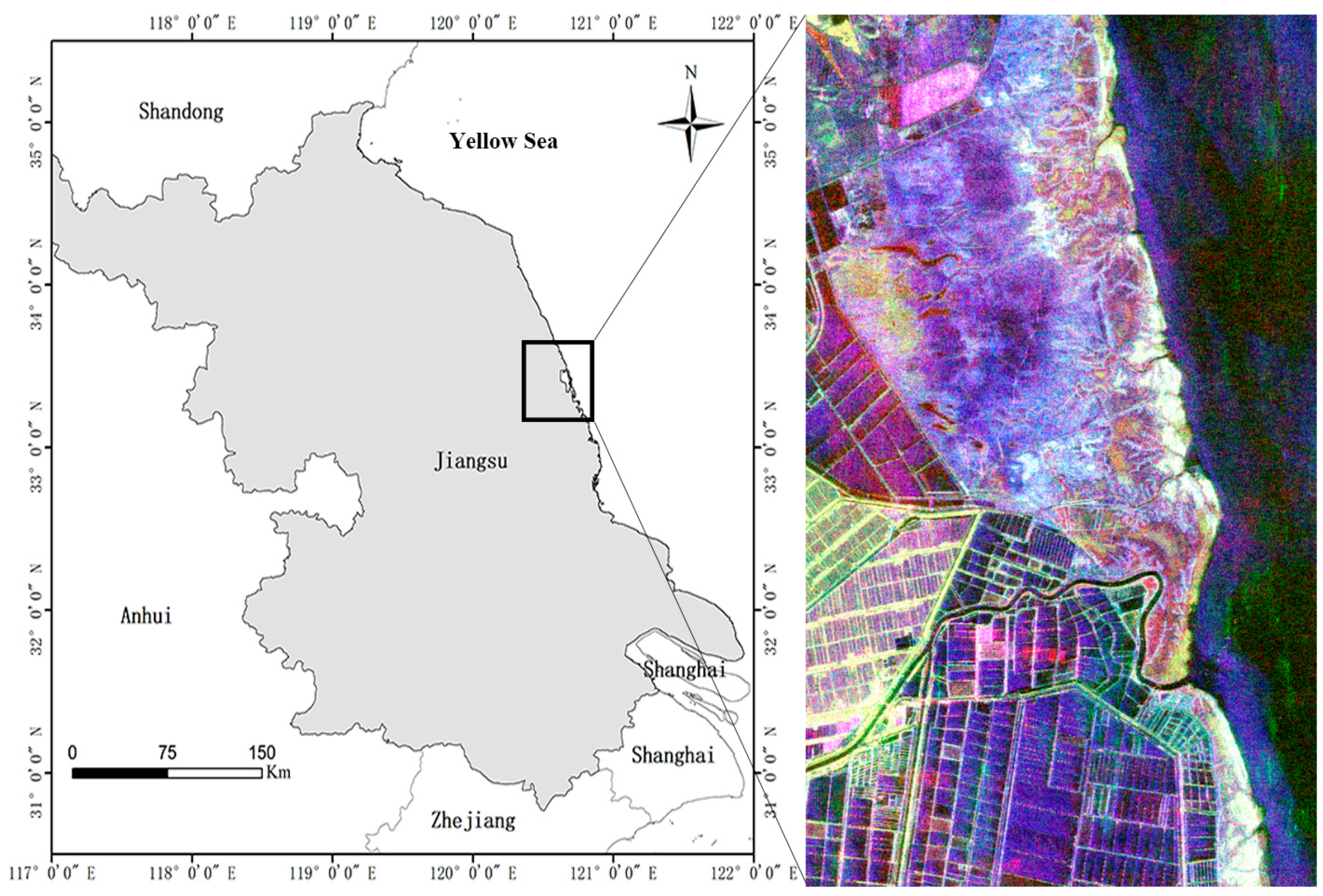
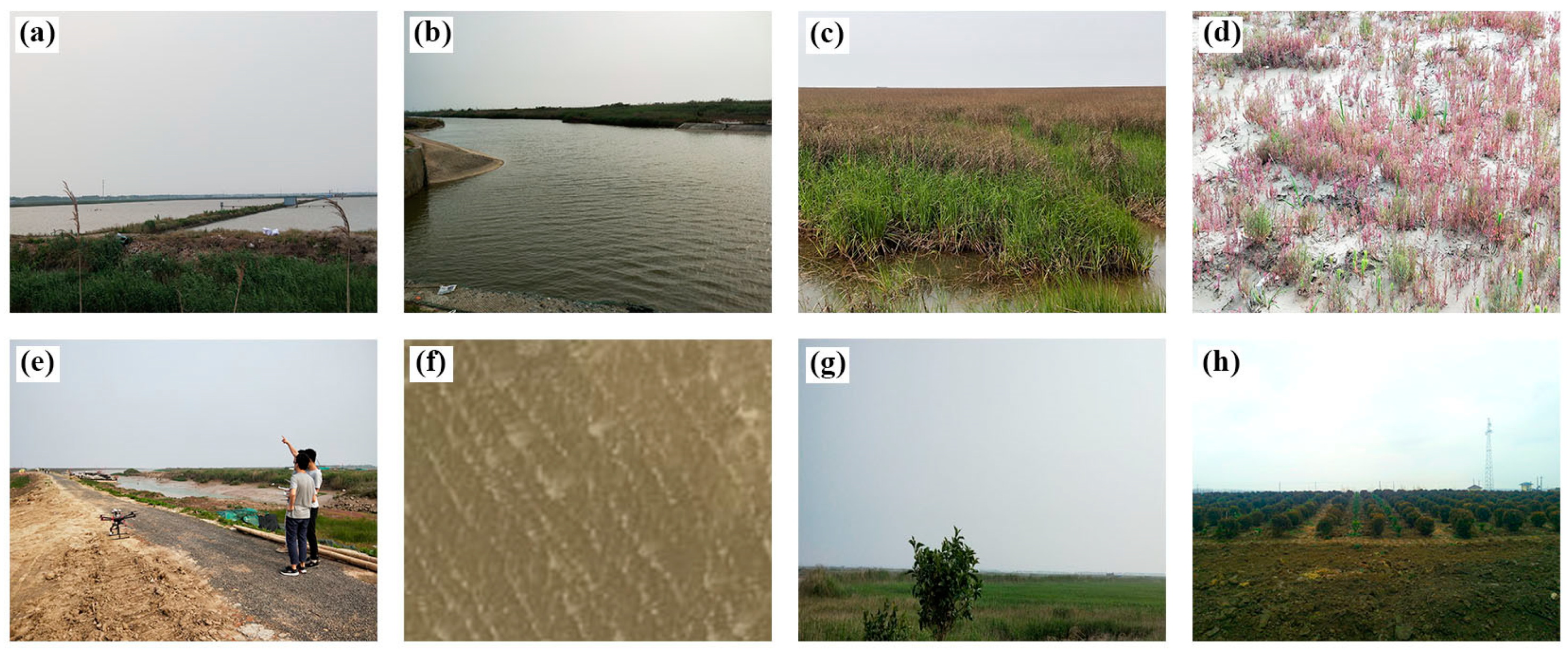
2.1. Study Area and Data

The experiment was conducted in the Jiangsu coastal area, which is located along the Yangtze River Basin in eastern China (Figure 1). The typical land cover types in the selected study area include sea, fish pond, irrigable land, reed and alterniflora, Suaeda salsa, rice paddy, river, road, and sand. Reed and alterniflora were classified into one category because the scattering characteristics of these two kinds of land covers were exactly similar, and the resolution of the used SAR data was relatively limited. Therefore, it was difficult to distinguish these two kinds of land covers in polarimetric SAR images, and these were thus regarded as a mixed land type.
L-band fully polarimetric ALOS PALSAR data with a resolution of 9.37 m × 3.57 m were used in the experiment. In addition, QuickBird high-resolution optical images and Google Earth images were simultaneously acquired as auxiliary data for visual interpretation of the results. The polarimetric SAR data was preprocessed with terrain correction, geocoding, multi-look, and filtering. Here, a multi-look processing with 6:1 in the azimuth direction and the range direction was applied to improve the image readability, and Refined Lee filtering with a 3 × 3 window size was employed to reduce noise [35]. A total of 44,961 sample points were collected during fieldwork, among which 28,654 were used for the random forest model construction and 16,307 for classification results validation. Some photographs of typical land covers were taken during the fieldwork (Figure 2). The setting of the sample points is shown in Table 1.

2.2. Polarimetric Scattering Features Extraction

2.2.1. Matrix Element Features

Scattering matrix, coherent matrix, and covariance matrix can all be used to represent polarimetric SAR data [36]. Each element in the matrix contains different polarimetric scattering information. Therefore, these matrix elements can be used for PolSAR classification. Equations (1)–(3) represent different matrix elements.
S = [ S h h S h v S h v S v v ]
T 3 = 1 2 [ | S h h + S v v | 2 ( S h h + S v v ) ( S h h S v v ) 2 ( S h h + S v v ) S h v ( S h h S v v ) ( S h h + S v v ) | S h h S v v | 2 2 ( S h h S v v ) S h v 2 S h v ( S h h + S v v ) 2 S h v ( S h h S v v ) 4 | S h v | 2 ]
C 3 = [ | S h h | 2 2 S h h S h v S h h S v v 2 S h v S h h 2 | S h v | 2 2 S h v S v v S v v S h h 2 S v v S h v | S v v | 2 ]
where S h h , S h v , and S v v are the elements of the polarimetric scattering matrix, is inner product operation, | | is determinant of a matrix, S v v represents the adjoint matrix of S v v ; the coherence matrix elements and the covariance matrix elements are obtained via the second-order operations of the scattering matrix elements. Each set of group elements of the three forms of matrices contains all the information in the full polarimetric SAR data. Therefore, using any group of matrix elements to participate in polarimetric scattering information extraction is equivalent to using any of the other groups for the same purpose [36]. In this study, three scattering matrix elements, S h h , S h v , and S v v , were employed in classification.

2.2.2. Polarimetric Decomposition Features

Polarimetric decomposition is an important scattering information extraction approach in polarimetric SAR data application [35,37]. As a well-known and basic decomposition, the Pauli decomposition expresses the backscattering matrix S with the so-called Pauli basis:
S = [ S h h S h v S v h S v v ] = a 2 [ 1 0 0 1 ] + b 2 [ 1 0 0 1 ] + c 2 [ 0 1 1 0 ] + d 2 [ 0 i i 0 ]
Here ,   a = S h h + S v v 2 , b = S h h S v v 2 , c = S h v + S v h 2 , d = i S h v S v h 2
where [ 1 0 0 1 ] , [ 1 0 0 1 ] , [ 0 1 1 0 ] , and [ 0 i i 0 ] are the Pauli basis, S h h , S h v , S v h , and S v v are the elements of the polarimetric scattering matrix. With the reciprocity theorem and S h v = S v h , the Pauli basis can be reduced to the first three matrices. S h h + S v v , S h h S v v , and 2 S h v are associated with physical scattering mechanisms, which are odd-scattering, even-scattering, and volume scattering, respectively [35]. The total power of the polarimetric SAR is obtained as follows:
S p a n = | S h h | 2 + 2 | S h v | 2 + | S v v | 2 = | a | 2 + | b | 2 + | c | 2
Thus, the Pauli image, where | a | 2 corresponds to blue band, | b | 2 corresponds to red band, and | c | 2 corresponds to green band, represents all information in a PolSAR data and can be utilized to visual interpretation [36].
In addition to Pauli decomposition, many other polarimetric decomposition algorithms have been proposed, each of which may have their inherent defects or deficiencies. Moreover, polarimetric features obtained from different decomposition algorithms have different sensitivities to land covers [35]. Therefore, integrating multiple polarimetric decomposition algorithms will be an effective way of making polarimetric SAR data more suitable for complex coastal environments [23,24]. In this study, 93 polarimetric scattering features were extracted by using the 20 polarimetric decomposition algorithms listed in Table 2, and a total of 96 polarimetric features were obtained by adding 3 scattering matrix elements. These 96 polarimetric parameters were combined into a multi-band image, and then object-oriented segmentation and classification were performed on the multi-band image.

2.3. Object-Oriented Method

In recent years, object-oriented methods have been increasingly applied in remote sensing image classification. Unlike pixel-based methods, object-oriented ideas consider not only the spectral properties (color) of pixels, but also the spatial connections of pixels (shape, texture, size, etc.), and treat some homogeneous pixels as an object [25,26,27]. The object is used as a unit for segmentation and classification, and thus the method is efficient, and the classification results are better matched with the real land covers. As the first step of object-oriented analysis, the result of image segmentation will directly affect the final classification performance [28]. Multi-scale segmentation, a more commonly used segmentation algorithm for object-oriented methods, is a bottom-up method that combines adjacent pixels or small segmentation objects [25]. This algorithm performs object delineation based on shape and color homogeneity and realizes image segmentation based on region merging technology under the premise of ensuring minimum average heterogeneity between objects and maximum homogeneity between internal pixels of objects. There are three parameters that are crucial to the effect of multi-scale segmentation, namely, image layer weights, scale parameter, and composition of homogeneity criterion.
When too many layers participate in segmentation, the processing speed will be very slow, and the noise in each polarimetric feature layer will also cause the blurring of segmentation results and the fragmentation of blocks. Like in this study, if all of the obtained 96 polarimetric scattering features participate in segmentation, the calculation amount will be too large, and the segmentation result will not be satisfactory. As noted, the Pauli image can represent all the information contained in a PolSAR image, and the three bands of the Pauli RGB image correspond to the physical scattering mechanism of the real land covers. It can be used to qualitatively analyze the physical significance of the land covers in the polarimetric SAR image. Therefore, the Pauli RGB image was adopted for multi-scale segmentation. Moreover, the three bands of the Pauli image correspond to three scattering mechanisms with the same importance, so equal weights were set for each band during the segmentation [54].
The scale parameter is used to determine the maximum allowed heterogeneity of the generated image object [55]. The larger the value of the scale, the larger the size of the generated image object, and vice versa. If the scale parameter is too small, the segmented objects will be too fragmented to reflect the shapes of the land covers; if the scale parameter is too large, the details of the land covers will be lost [56,57]. Homogeneity is used to represent the minimum heterogeneity and consists of two parts, namely color (spectrum) and shape, the weights of which add up to 1.0. Furthermore, the shape is represented by smoothness and compactness, the weights of which also add up to 1.0. The color and shape, and the smoothness and compactness, can be regarded as the "opposite value" to each other. If the shape of the land cover in the image can indeed reflect its characteristics, the weight of the shape can be appropriately increased, while that of color can be reduced. Smoothness represents the smoothness of the edge of the segmented object, and compactness represents the tightness of the whole segmented object. In the process of segmentation, the optimal scale parameter and homogeneity criterion are usually determined by multiple trials [23]. The criterion to evaluate the segmentation result is whether the segmentation object is large enough and contains only one category.

2.4. Random Forest and Feature Set Optimization

Random forest (RF) is a machine learning model developed in recent years. The theoretical basis of the model is the decision tree; RF is obtained by combining different decision trees [30,31]. In other words, many decision trees { h ( X , θ k ) , k = 1 , } are generated via the randomization of variables and data, and there is no connection between each tree. The parameter set θ k is an independent random vector with the same distribution. When the independent variable X is given, each decision tree uses the voting method to produce the optimal result. When original data are entered into the random forest model, each decision tree classifies the data. The final result is the classification result which appears most frequently in all trees.
In the process of random forest model training, the importance of each variable can be calculated [32,33,34]. There are two types of importance measures: mean decrease impurity and mean decrease accuracy (MDA). The former is a calculating method of the Gini index, and the latter is a calculating method based on OOB (out-of-bag) error [58,59]. Here, the MDA method is employed. This method directly measures the effect of each feature on the accuracy of model prediction. The basic idea is to rearrange the order of a certain column of feature values and to observe how much the model accuracy is reduced. For non-important features, this method has little effect on the accuracy of the model, but for important features, it can greatly reduce the accuracy of the model. That is, when random white noise is added to a feature, observing the effect on the accuracy of the result. A small influence means that this feature is not important, otherwise it is important. The calculation of the importance of a feature f in a random forest is as follows:
Step 1. For each decision tree in a random forest, use the corresponding OOB (out-of-bag) data to calculate its out-of-bag data error, and record it as errOOB1;
Step 2. Randomly add noise to the feature f of all samples of the OOB data outside the bag, and calculate the error of the data outside the bag again, and record it as errOOB2;
Step 3. Assuming there are N trees in the random forest, the importance for feature f can be calculated as follows:
I M = 1 N i = 1 N ( e r r O O B 2 e r r O O B 1 )
where IM is the importance of feature f . The larger the IM value of a given feature, the more important it is.
In this study, the importance values of polarimetric features extracted from 20 decomposition algorithms were calculated by utilizing random forest models; these feature parameters were then sorted from high to low according to their importance values. In the process of feature set optimization, sequential forward selection (SFS) algorithm was adopted [60]. The idea is as follows: If the original feature set is F and the current feature set is X , which contains n features, for each feature f i that is not selected for X (i.e., the remaining features after X is removed from F ), the overall classification accuracy is calculated after introducing the feature into feature set X , and the optimal polarimetric feature is selected according to the overall accuracy of each calculation. That is, the feature subset corresponding to the highest classification overall accuracy is selected as the optimal set. The optimal feature subset has the least number of polarimetric parameters and the highest classification accuracy. As the sequential forward selection algorithm is employed to calculate the overall classification accuracy under all feature sets, and the feature set corresponding with the highest classification accuracy is selected, it will not fall into the local optimal solution. The process of optimizing the polarimetric scattering feature set using the RF-SFS algorithm is shown in Figure 3.

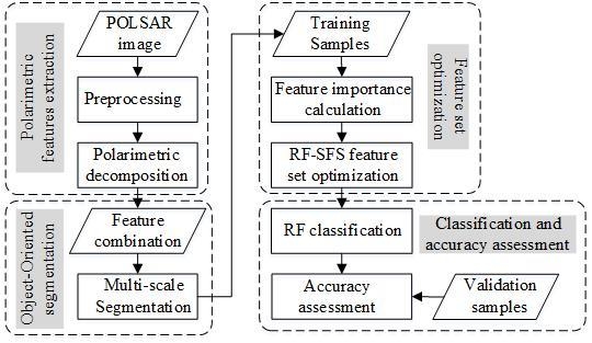
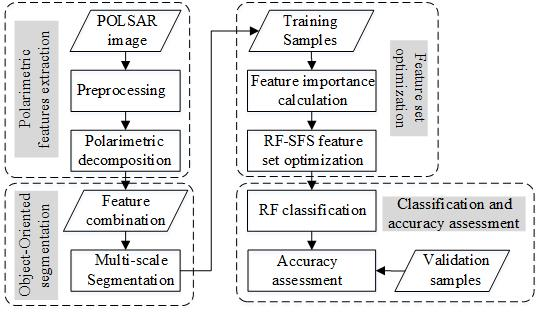
2.5. Experimental Flowchart
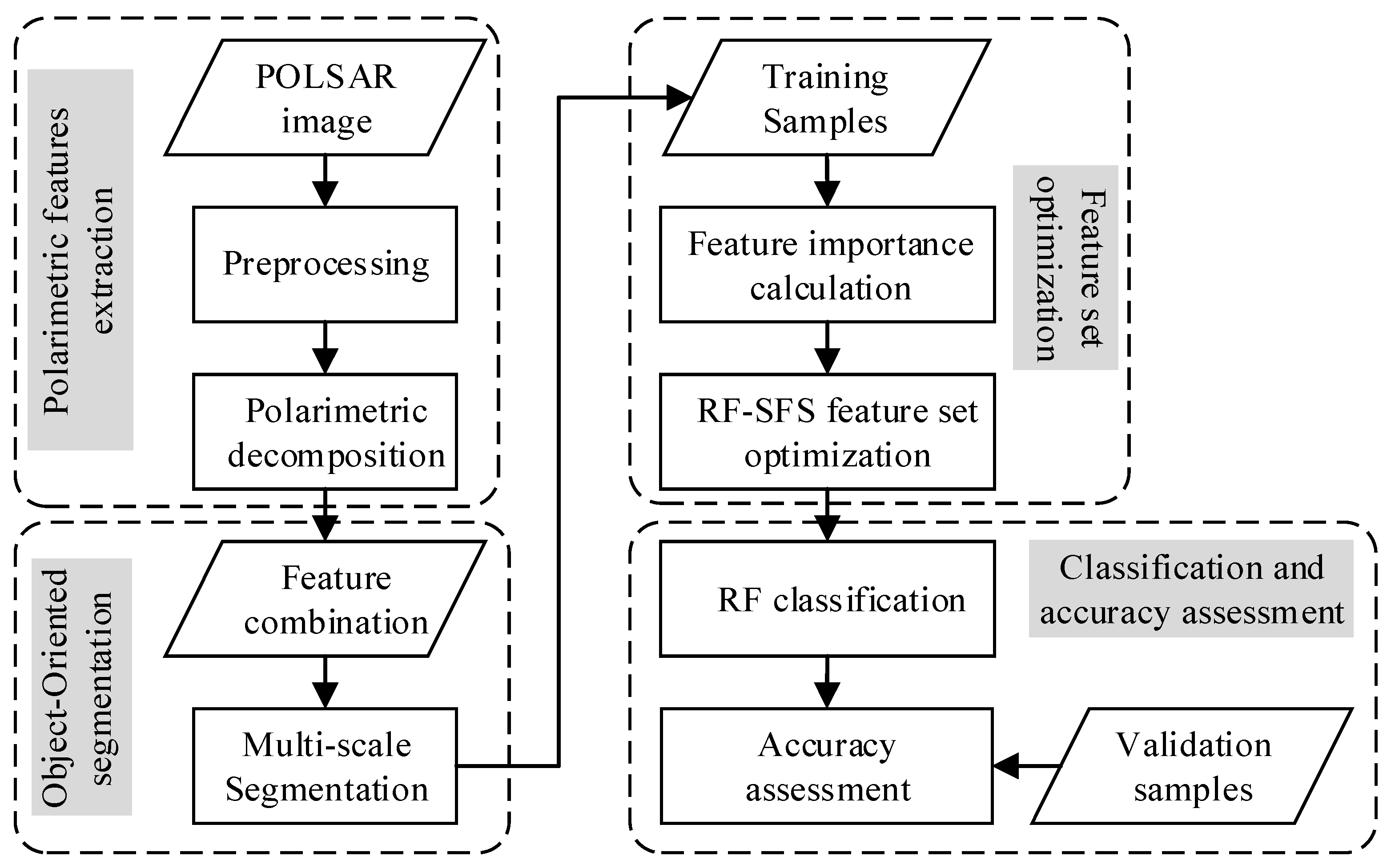
In this research, the object-oriented RF-SFS algorithm, which is a feature set optimization and classification method combining random forest (RF) model and sequential forward selection (SFS), was proposed. The specific processes of this method are as follows:
(1)
Filtering and other preprocessing were applied to the original polarimetric SAR data;
(2)
Twenty polarimetric decompositions listed in Table 2 were utilized to decompose the filtered coherent matrix, and 93 polarimetric decomposition features were obtained. Three scattering matrix elements, S11, S12 and S22, were used as matrix features, and thus a total of 96 polarimetric scattering features could be obtained;
(3)
The scattering features obtained from the previous step were combined into a multi-band image, to which object-oriented multi-scale segmentation was then performed;
(4)
Training samples based on the segmented object as the basic unit were randomly selected;
(5)
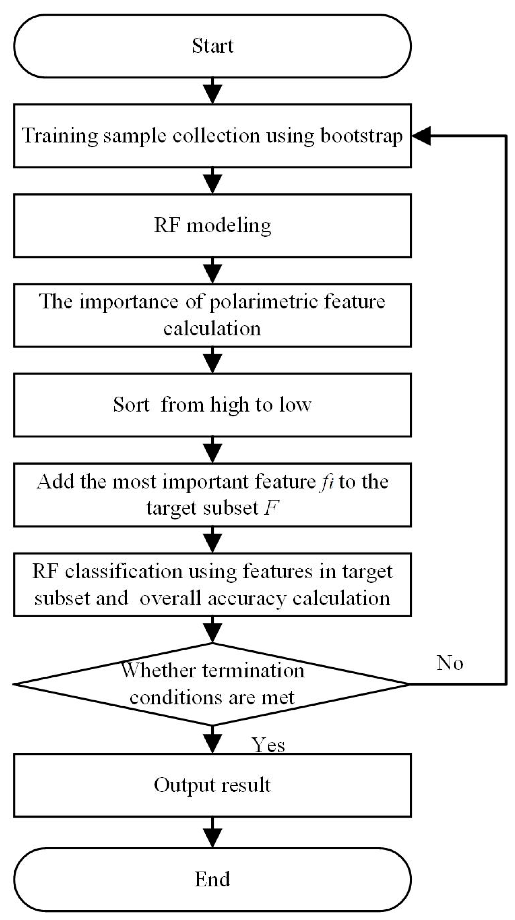
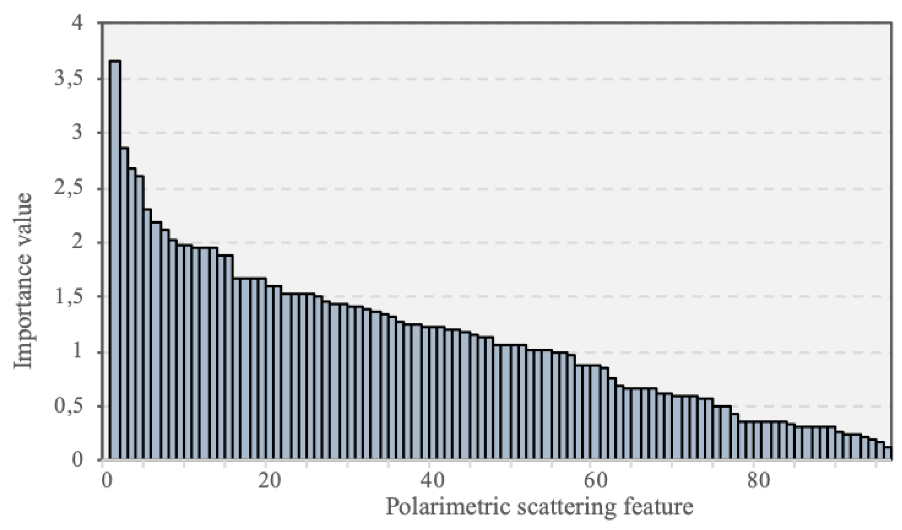
Formula (7) was used to calculate the importance of all polarimetric scattering features of training samples;
(6)
The features were ranked according to the importance value;
(7)
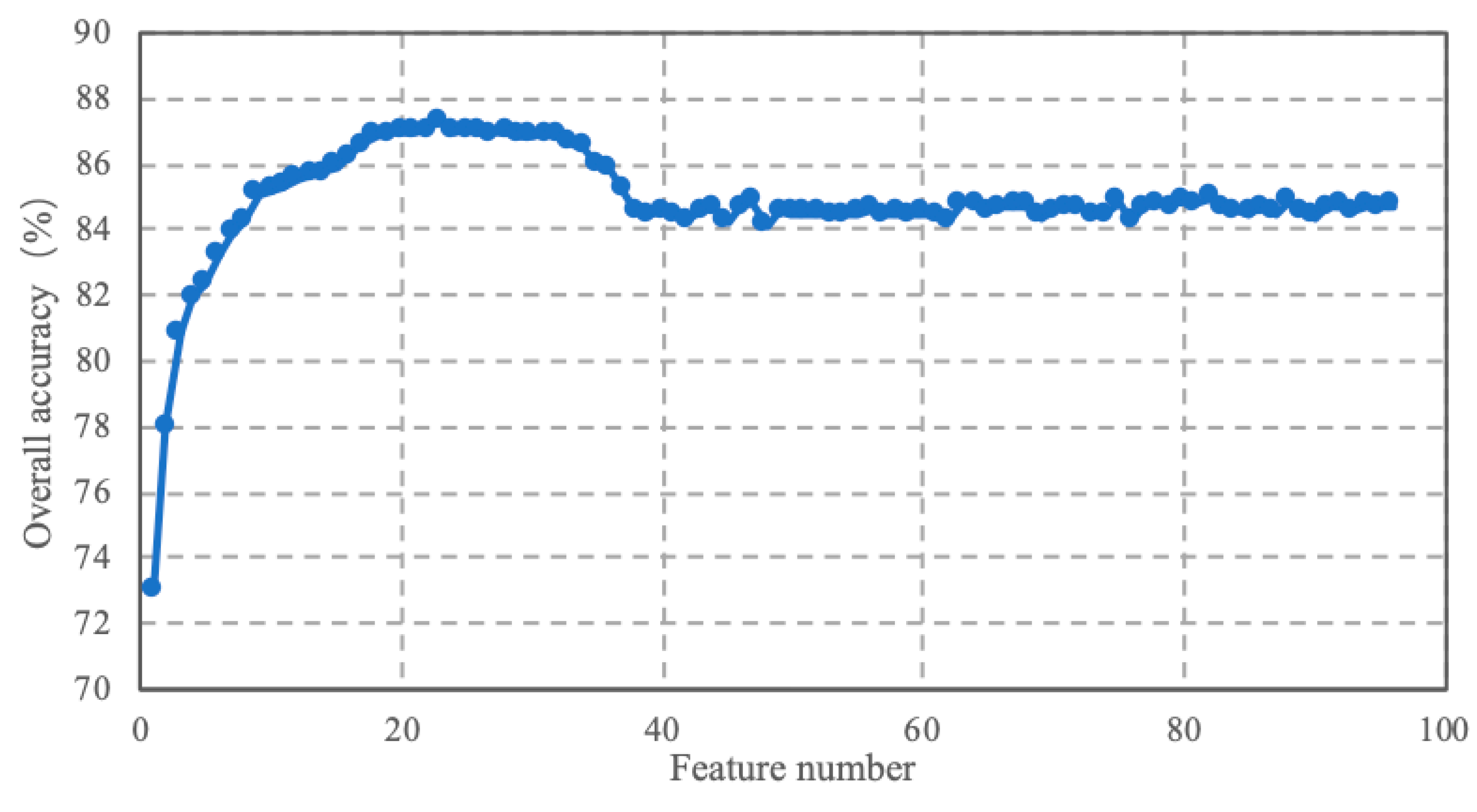
Using the sequential forward selection algorithm to optimize the feature set, the feature subset with the least number of features and the highest classification accuracy was obtained;
(8)
The selected optimal polarimetric feature subset was classified based on the object-oriented random forest model;
(9)
The classification accuracy was calculated by using validation samples.
A flowchart of the proposed methodology is given in Figure 4.

3. Results and Discussion

3.1. Importance Analysis of Polarimetric Features and Feature Set Optimization

The importance values of the 96 polarimetric scattering features were calculated using Formula (7), as listed in Table 3. The importance values were ranked in descending order, as displayed in Figure 5. As previously stated, the larger the IM value of a given feature, the more important it is. From Table 3 and Figure 5, we can see the importance value of each feature and can know which features are more important for the experimental results. However, different combinations of features will produce different results when participating in classification. Therefore, determining which polarimetric features are selected for classification to obtain the highest classification accuracy is the next problem to be solved.
For the feature set composed of 96 polarimetric features, the RF-SFS algorithm proposed in this study was adopted to optimize the feature set according to the importance value of each feature. Assuming the initial target feature subset was empty, the specific method was to add the feature with the highest importance value to the target feature subset each time, and then the features in the target subset were performed to classification and the overall accuracy of the result was calculated, and iterate iteratively until all features were added to the target subset and the accuracy was calculated. The relationship between the classification accuracy calculated by each iteration and the number of polarimetric features is shown in Figure 6. As can be seen from the figure, for the features that ranked in the first nine in terms of importance, the classification accuracy was greatly improved for each additional feature. After the number of features increased to nine, the classification accuracy changed slowly. When the number increased to 23, the classification accuracy reached its highest value, which was 87.29%. After that, the number of features increased, and the overall accuracy did not change significantly. Even when the number of features reached 38, the classification accuracy was slightly reduced, and was about 2.5% lower than the accuracy of the 23 features participating in the classification. Furthermore, as the number of features participating in the classification increased, the computational burden also increased. This result indicates that when too many polarimetric features are involved in the classification, the computational burden will be aggravated, and the information redundancy between features will reduce the classification effect. Therefore, the classification is based on the first 23 polarimetric features in the importance ranking. This ensures the accuracy of the classification results and avoids the redundancy of information between features.
From Table 3 and Figure 5, it is also easy to see that among the top 23 polarimetric features with the higher importance values, S h h , S h v , and S v v are three scattering matrix elements; Entropy_shannon, Entropy, Lambda, HAA_T11, Pedestal, and Alpha are six polarimetric features from H / α decomposition; Yamaguchi3_Dbl and Yamaguchi3_Odd are two polarimetric features from Yamaguchi3 decomposition; VanZyl3_Dbl and VanZyl3_Vol are two polarimetric features from VanZyl3 decomposition; Krogager_Kd and Krogager_Ks are two polarimetric features from Krogager decomposition. A total of 15 of the first 23 features are derived from the scattering matrix and the above four polarimetric decomposition methods. In other words, the features obtained by the aforementioned algorithms account for more than 65% of the total number of the first 23 important features, indicating that these features are more important, and these decomposition algorithms have obvious advantages over other decomposition methods in coastal wetland classification.

3.2. Classification Results

In this research, the following three methods were used to conduct comparative experiments in the study area: (a) the proposed method; (b) QUEST decision tree algorithm without artificial pruning; and (c) QUEST decision tree algorithm with artificial pruning. In method (b), the tree depth was not set manually, and the decision tree grew freely. In method (c), in order to prevent overfitting caused by the infinite growth of the decision tree, the tree depth was set to 5. The classification results of these three methods are shown in Figure 7. In addition, the user’s accuracy (UA), the producer’s accuracy (PA), the overall accuracy (OA), and the Kappa coefficient of the three classification results were calculated for quantitative analysis, as shown in Table 4, Table 5 and Table 6.

3.3. Discussion

The decision tree is a tree built on the basis of decision choices. It is simple to implement and is widely used in remote sensing classification [54,61]. It summarizes the training data set, learns to form a series of rule sets, and classifies the pixels or groups of remote sensing image data according to the generated rule sets. Sometimes the tree is too "lush", that is, there are too many nodes and overfitting may occur during the tree building process. Therefore, artificial pruning needs to be performed to remove some unnecessary branches. The author’s previous research has proved the effectiveness of the QUEST decision tree algorithm in the classification of coastal wetlands [23]. However, it required artificial pruning of the tree and did not provide a method for quantitatively evaluating the validity of features. Random forests are obtained by combining decision trees, and its theoretical basis is decision trees. In theory, the classification results using multiple trees are better than a single tree. This research will also prove this through comparative experiments.
By comparing the experimental results, the overall accuracy of the classification results obtained by the object-oriented RF-SFS method was improved by more than 11% and the Kappa coefficient increased by 0.14 compared with those of the object-oriented QUEST decision tree method without artificial pruning. As shown in the boxed area of the figure, when the QUEST decision tree method without artificial pruning was adopted, some sporadic plots in the alterniflora region were divided into rice paddy and fish ponds, and some Suaeda salsa areas were not properly separated. The classification accuracy for these wetland land covers was lower than that of the proposed algorithm. In addition, the Suaeda salsa in the elliptical area was not completely identified, and most of these regions were mistakenly classified as alterniflora, and some Suaeda salsa areas that were closer to the sea were misclassified into irrigated land. Relatively satisfactory classification results were obtained for the aforementioned wetland types when the proposed method was used. As shown in Table 4, the user’s and producer’s accuracies for Suaeda salsa were 84.86% and 80.78%, respectively. For irrigable land, the two indicators were 87.89% and 77.65%, respectively. When the QUEST decision tree method without artificial pruning was performed, as shown in Table 5, the user’s accuracies of Suaeda salsa and irrigable land were 61.37% and 75.39%, respectively, which were 23.49% and 12.5%, respectively, lower than that of the proposed method. Meanwhile, the producer’s accuracies for these two land types were 72.90% and 57.06%, respectively, which were significantly lower than that of the proposed method. When artificial pruning was performed on the QUEST decision tree, as shown in Figure 7c and Table 6, the user’s and producer’s accuracies for Suaeda salsa were 80.69% and 77.16%, respectively, and the two indicators of irrigated land were 79.00% and 67.14%, respectively. These indicators were all improved compared with those for the algorithm without artificial pruning operation, but were still lower than the accuracy obtained by the algorithm proposed in this research. Through the comparison, it was found that some fish ponds in the results for the method without artificial pruning were misclassified into sea, and some paddy fields were mistakenly divided into irrigated land, as shown in Figure 7b. The results of the cases of misclassification for these wetland land covers have been improved after artificial pruning. However, compared with the results of the proposed method, there were still small blocks that were misclassified and the accuracy was still lower, as shown in Figure 7c and Table 6. It can be seen that the object-oriented RF-SFS method not only had certain advantages in the optimization of polarimetric feature set, but also achieved high classification accuracy without artificial pruning in the modeling process.

4. Conclusions

A single polarimetric decomposition has difficulty in mining all the scattering information contained in a PolSAR image. The decision tree method requires artificial pruning and cannot quantitatively evaluate the validity of features. Therefore, this research proposed a feature set optimization and polarimetric SAR image classification method that integrates multiple polarimetric decompositions, random forest model, and sequence forward selection algorithm, namely, the RF-SFS algorithm for land cover classification in coastal wetlands using fully polarimetric ALOS PALSAR data. The following conclusions can be drawn through a comparative analysis of the experiment:
(1)
The proposed method calculated the importance of each polarimetric feature in the construction of a random forest model, and the sequence forward selection algorithm was applied to select the optimal polarimetric feature set that is suitable for Jiangsu coastal wetlands classification according to the importance value. This method provided a quantitative reference for the reasonable optimization of feature sets;
(2)
The importance values of features from the scattering matrix and the four decomposition algorithms, namely, H / α decomposition, Yamaguchi3 decomposition, VanZyl3 decomposition, and Krogager decomposition, were higher than other features. This indicated that these features were more important and were determined to be very supportive of land cover identification in the Jiangsu coastal wetlands;
(3)
Compared with the object-oriented QUEST decision tree algorithm, regardless of whether the latter has been pruned, the proposed object-oriented RF-SFS method can achieve higher classification accuracies without artificial pruning.
Overall, the findings in this study demonstrated that the proposed object-oriented RF-SFS algorithm significantly contributes to coastal wetlands classification when using fully polarimetric ALOS PALSAR data. However, as the scattering characteristics of these two kinds of land covers were exactly similar, and the resolution of the used SAR data was relatively limited, reed and alterniflora were classified into one category in this research. Future studies should be conducted that include employing other novel classification algorithms or integrating of optical and SAR data to distinguish these two kinds of land covers.

Author Contributions

Conceptualization, Y.C.; Formal analysis, J.X.; Funding acquisition, Y.C.; Investigation, Y.C., R.Z. and Y.L.; Methodology, Y.C. and X.H.; Project administration, X.H.; Resources, X.H.; Software, J.X.; Supervision, X.H.; Validation, Y.C. and Y.L.; Visualization, Y.C., J.X., R.Z. and Y.L.; Writing—original draft, Y.C. and J.X.; Writing—review & editing, R.Z. and Y.L. All authors have read and agreed to the published version of the manuscript.

Funding

This research was supported by the Research Project of Surveying Mapping and Geoinformation of Jiangsu Province (Grant No. JSCHKY201708), the Natural Science Foundation of Jiangsu Province (Grant No. BK20180779), the Youth Science and Technology Innovation Fund Project of Nanjing Forestry University (Grant No. CX2018015), and the National Natural Science Foundation of China (Grant No. 41830110, 41901401).

Acknowledgments

The ALOS PALSAR imagery was provided by the Japan Aerospace Exploration Agency.

Conflicts of Interest

The authors declare no conflict of interest.

References

  1. Michener, W.K.; Blood, E.R.; Bildstein, K.L.; Brinson, M.M.; Gardner, L.R. Climate change, hurricanes and tropical storms, and rising sea level in coastal wetlands. Ecol. Appl. 1997, 7, 770–801. [Google Scholar] [CrossRef]
  2. Costanza, R.; Pérez-Maqueo, O.; Martinez, M.L.; Sutton, P.; Anderson, S.J.; Mulder, K. The value of coastal wetlands for hurricane protection. Ambio 2008, 37, 241–249. [Google Scholar] [CrossRef]
  3. Perillo, G.; Wolanski, E.; Cahoon, D.R.; Hopkinson, C.S. Coastal Wetlands: An Integrated Ecosystem Approach; Elsevier: Amsterdam, The Netherlands, 2018. [Google Scholar]
  4. Prince, H.H. Coastal Wetlands; CRC Press: Boca Raton, FL, USA, 2018. [Google Scholar]
  5. Sievers, M.; Brown, C.J.; Tulloch, V.J.; Pearson, R.M.; Haig, J.A.; Turschwell, M.P.; Connolly, R.M. The role of vegetated coastal wetlands for marine megafauna conservation. Trends Ecol. Evol. 2019, 34, 807–817. [Google Scholar] [CrossRef] [PubMed]
  6. Hardisky, M.; Gross, M.; Klemas, V. Remote sensing of coastal wetlands. Bioscience 1986, 36, 453–460. [Google Scholar] [CrossRef]
  7. Klemas, V. Remote sensing of wetlands: Case studies comparing practical techniques. J. Coast. Res. 2011, 27, 418–427. [Google Scholar]
  8. Doughty, C.L.; Cavanaugh, K.C. Mapping Coastal Wetland Biomass from High Resolution Unmanned Aerial Vehicle (UAV) Imagery. Remote Sens. 2019, 11, 540. [Google Scholar] [CrossRef] [Green Version]
  9. Verstraete, M.M.; Pinty, B.; Myneni, R.B. Potential and limitations of information extraction on the terrestrial biosphere from satellite remote sensing. Remote Sens. Environ. 1996, 58, 201–214. [Google Scholar] [CrossRef]
  10. Adam, E.; Mutanga, O.; Rugege, D. Multispectral and hyperspectral remote sensing for identification and mapping of wetland vegetation: A review. Wetl. Ecol. Manag. 2010, 18, 281–296. [Google Scholar] [CrossRef]
  11. Kasischke, E.S.; Bourgeau-Chavez, L.L. Monitoring South Florida wetlands using ERS-1 SAR imagery. Photogramm. Eng. Remote Sens. 1997, 63, 281–291. [Google Scholar]
  12. White, L.; Brisco, B.; Dabboor, M.; Schmitt, A.; Pratt, A. A collection of SAR methodologies for monitoring wetlands. Remote Sens. 2015, 7, 7615–7645. [Google Scholar] [CrossRef] [Green Version]
  13. Mohammadimanesh, F.; Salehi, B.; Mahdianpari, M.; Brisco, B.; Motagh, M. Multi-temporal, multi-frequency, and multi-polarization coherence and SAR backscatter analysis of wetlands. ISPRS-J. Photogramm. Remote Sens. 2018, 142, 78–93. [Google Scholar] [CrossRef]
  14. Amani, M.; Salehi, B.; Mahdavi, S.; Brisco, B. Separability analysis of wetlands in Canada using multi-source SAR data. GISci. Remote Sens. 2019, 56, 1233–1260. [Google Scholar] [CrossRef]
  15. Choe, B.-H.; Kim, D.-j.; Hwang, J.-H.; Oh, Y.; Moon, W.M. Detection of oyster habitat in tidal flats using multi-frequency polarimetric SAR data. Estuar. Coast. Shelf Sci. 2012, 97, 28–37. [Google Scholar] [CrossRef]
  16. Chauhan, S.; Srivastava, H.S. Comparative evaluation of the sensitivity of multi-polarized SAR and optical data for various land cover classes. Int. J. Adv. Remote Sens. GIS Geogr 2016, 4, 1–14. [Google Scholar]
  17. Pereira, L.; Furtado, L.; Novo, E.; Sant’Anna, S.; Liesenberg, V.; Silva, T. Multifrequency and Full-Polarimetric SAR Assessment for Estimating Above Ground Biomass and Leaf Area Index in the Amazon Várzea Wetlands. Remote Sens. 2018, 10, 1355. [Google Scholar] [CrossRef] [Green Version]
  18. Millard, K.; Richardson, M. Wetland mapping with LiDAR derivatives, SAR polarimetric decompositions, and LiDAR–SAR fusion using a random forest classifier. Can. J. Remote Sens. 2013, 39, 290–307. [Google Scholar] [CrossRef]
  19. de Almeida Furtado, L.F.; Silva, T.S.F.; de Moraes Novo, E.M.L. Dual-season and full-polarimetric C band SAR assessment for vegetation mapping in the Amazon várzea wetlands. Remote Sens. Environ. 2016, 174, 212–222. [Google Scholar] [CrossRef] [Green Version]
  20. Hong, S.-H.; Kim, H.-O.; Wdowinski, S.; Feliciano, E. Evaluation of polarimetric SAR decomposition for classifying wetland vegetation types. Remote Sens. 2015, 7, 8563–8585. [Google Scholar] [CrossRef] [Green Version]
  21. Chen, Y.; He, X.; Wang, J. Classification of coastal wetlands in eastern China using polarimetric SAR data. Arab. J. Geosci. 2015, 8, 10203–10211. [Google Scholar] [CrossRef]
  22. Touzi, R.; Deschamps, A.; Rother, G. Wetland characterization using polarimetric RADARSAT-2 capability. Can. J. Remote Sens. 2007, 33, S56–S67. [Google Scholar] [CrossRef]
  23. Chen, Y.; He, X.; Wang, J.; Xiao, R. The influence of polarimetric parameters and an object-based approach on land cover classification in coastal wetlands. Remote Sens. 2014, 6, 12575–12592. [Google Scholar] [CrossRef] [Green Version]
  24. Niu, X.; Ban, Y. Multi-temporal RADARSAT-2 polarimetric SAR data for urban land-cover classification using an object-based support vector machine and a rule-based approach. Int. J. Remote Sens. 2013, 34, 1–26. [Google Scholar] [CrossRef]
  25. Blaschke, T. Object based image analysis for remote sensing. ISPRS-J. Photogramm. Remote Sens. 2010, 65, 2–16. [Google Scholar] [CrossRef] [Green Version]
  26. Blaschke, T.; Lang, S.; Hay, G. Object-Based Image Analysis: Spatial Concepts for Knowledge-Driven Remote Sensing Applications; Springer Science & Business Media: Berlin/Heidelberg, Germany, 2008. [Google Scholar]
  27. Ma, L.; Li, M.; Ma, X.; Cheng, L.; Du, P.; Liu, Y. A review of supervised object-based land-cover image classification. ISPRS-J. Photogramm. Remote Sens. 2017, 130, 277–293. [Google Scholar] [CrossRef]
  28. Ban, Y.; Hu, H.; Rangel, I.M. Fusion of Quickbird MS and RADARSAT SAR data for urban land-cover mapping: Object-based and knowledge-based approach. Int. J. Remote Sens. 2010, 31, 1391–1410. [Google Scholar] [CrossRef]
  29. Fu, B.; Wang, Y.; Campbell, A.; Li, Y.; Zhang, B.; Yin, S.; Xing, Z.; Jin, X. Comparison of object-based and pixel-based Random Forest algorithm for wetland vegetation mapping using high spatial resolution GF-1 and SAR data. Ecol. Indic. 2017, 73, 105–117. [Google Scholar] [CrossRef]
  30. Liaw, A.; Wiener, M. Classification and regression by randomForest. R. News 2002, 2, 18–22. [Google Scholar]
  31. Pal, M. Random forest classifier for remote sensing classification. Int. J. Remote Sens. 2005, 26, 217–222. [Google Scholar] [CrossRef]
  32. Boonprong, S.; Cao, C.; Chen, W.; Bao, S. Random Forest Variable Importance Spectral Indices Scheme for Burnt Forest Recovery Monitoring—Multilevel RF-VIMP. Remote Sens. 2018, 10, 807. [Google Scholar] [CrossRef] [Green Version]
  33. Belgiu, M.; Drăguţ, L. Random forest in remote sensing: A review of applications and future directions. ISPRS-J. Photogramm. Remote Sens. 2016, 114, 24–31. [Google Scholar]
  34. Lebourgeois, V.; Dupuy, S.; Vintrou, É.; Ameline, M.; Butler, S.; Bégué, A. A combined random forest and OBIA classification scheme for mapping smallholder agriculture at different nomenclature levels using multisource data (simulated Sentinel-2 time series, VHRS and DEM). Remote Sens. 2017, 9, 259. [Google Scholar] [CrossRef] [Green Version]
  35. Lee, J.-S.; Pottier, E. Polarimetric Radar Imaging: From Basics to Applications; CRC press: Boca Raton, FL, USA, 2009. [Google Scholar]
  36. Cloude, S.R.; Pottier, E. A review of target decomposition theorems in radar polarimetry. IEEE Trans. Geosci. Remote Sens. 1996, 34, 498–518. [Google Scholar] [CrossRef]
  37. Cloude, S.R.; Pottier, E. An entropy based classification scheme for land applications of polarimetric SAR. IEEE Trans. Geosci. Remote Sens. 1997, 35, 68–78. [Google Scholar] [CrossRef]
  38. Krogager, E. New decomposition of the radar target scattering matrix. Electron. Lett. 1990, 26, 1525–1527. [Google Scholar] [CrossRef]
  39. Huynen, J.R. Stokes matrix parameters and their interpretation in terms of physical target properties. In Proceedings of the Polarimetry: Radar, infrared, visible, ultraviolet, and X-ray, Nantes, France, 20–22 March 1990. [Google Scholar]
  40. Barnes, R. Roll-invariant decompositions for the polarization covariance matrix. In Proceedings of the Polarimetry Technology Workshop, Redstone Arsenal, AL, USA, 16–18 August 1988. [Google Scholar]
  41. Holm, W.A.; Barnes, R.M. On radar polarization mixed target state decomposition techniques. In Proceedings of the 1988 IEEE National Radar Conference, Ann Arbor, MI, USA, 20–21 April 1988; pp. 249–254. [Google Scholar]
  42. van Zyl, J.J. Application of Cloude’s target decomposition theorem to polarimetric imaging radar data. Radar Polarim. 1993, 1748, 184–191. [Google Scholar]
  43. Pottier, E.; Lee, J.-S. Application of the «H/A/alpha» polarimetric decomposition theorem for unsupervised classification of fully polarimetric SAR data based on the wishart distribution. In Proceedings of the SAR workshop: CEOS Committee on Earth Observation Satellites, Toulouse, France, 26–29 October 1999; pp. 335–340. [Google Scholar]
  44. Freeman, A. Fitting a two-component scattering model to polarimetric SAR data from forests. IEEE Trans. Geosci. Remote Sens. 2007, 45, 2583–2592. [Google Scholar] [CrossRef]
  45. Freeman, A.; Durden, S.L. A three-component scattering model for polarimetric SAR data. IEEE Trans. Geosci. Remote Sens. 1998, 36, 963–973. [Google Scholar] [CrossRef] [Green Version]
  46. Yamaguchi, Y.; Singh, G.; Yi, C.; Park, S.E.; Yamada, H.; Sato, R. Comparison of model-based four-component scattering power decompositions. In Proceedings of the 2013 Asia-Pacific Conference on Synthetic Aperture Radar (APSAR), Tsukuba, Japan, 23–27 September 2013; pp. 92–95. [Google Scholar]
  47. Yamaguchi, Y.; Moriyama, T.; Ishido, M.; Yamada, H. Four-component scattering model for polarimetric SAR image decomposition. IEEE Trans. Geosci. Remote Sens. 2005, 43, 1699–1706. [Google Scholar] [CrossRef]
  48. Neumann, M.; Ferro-Famil, L.; Pottier, E. A general model-based polarimetric decomposition scheme for vegetated areas. In Proceedings of the 4th International Workshop on Science and Applications of SAR Polarimetry and Polarimetric Interferometry-PolInSAR, Frascati, Italy, 26–30 January 2009. [Google Scholar]
  49. Touzi, R. Target scattering decomposition in terms of roll-invariant target parameters. IEEE Trans. Geosci. Remote Sens. 2006, 45, 73–84. [Google Scholar] [CrossRef]
  50. An, W.; Cui, Y.; Yang, J. Three-component model-based decomposition for polarimetric SAR data. IEEE Trans. Geosci. Remote Sens. 2010, 48, 2732–2739. [Google Scholar]
  51. An, W.; Xie, C.; Yuan, X.; Cui, Y.; Yang, J. Four-component decomposition of polarimetric SAR images with deorientation. IEEE Geosci. Remote Sens. Lett. 2011, 8, 1090–1094. [Google Scholar] [CrossRef]
  52. Arii, M.; van Zyl, J.J.; Kim, Y. Adaptive model-based decomposition of polarimetric SAR covariance matrices. IEEE Trans. Geosci. Remote Sens. 2010, 49, 1104–1113. [Google Scholar] [CrossRef]
  53. Arii, M.; van Zyl, J.; Kim, Y. Improvement of adaptive-model based decomposition with polarization orientation compensation. In Proceedings of the 2012 IEEE International Geoscience and Remote Sensing Symposium (IGARSS), Munich, Germany, 22–27 July 2012; pp. 95–98. [Google Scholar]
  54. Qi, Z.; Yeh, A.G.-O.; Li, X.; Lin, Z. A novel algorithm for land use and land cover classification using RADARSAT-2 polarimetric SAR data. Remote Sens. Environ. 2012, 118, 21–39. [Google Scholar] [CrossRef]
  55. Addink, E.A.; De Jong, S.M.; Pebesma, E.J. The importance of scale in object-based mapping of vegetation parameters with hyperspectral imagery. Photogramm. Eng. Remote Sens. 2007, 73, 905–912. [Google Scholar] [CrossRef]
  56. Anders, N.S.; Seijmonsbergen, A.C.; Bouten, W. Segmentation optimization and stratified object-based analysis for semi-automated geomorphological mapping. Remote Sens. Environ. 2011, 115, 2976–2985. [Google Scholar] [CrossRef]
  57. Kavzoglu, T.; Yildiz, M. Parameter-based performance analysis of object-based image analysis using aerial and Quikbird-2 images. In Proceedings of the ISPRS Annals of the Photogrammetry, Remote Sensing and Spatial Information Sciences, Istanbul, Turkey, 29 September–2 October 2014; pp. 31–37. [Google Scholar]
  58. Mitchell, M.W. Bias of the Random Forest out-of-bag (OOB) error for certain input parameters. Open J. Statist. 2011, 1, 205. [Google Scholar] [CrossRef] [Green Version]
  59. Millard, K.; Richardson, M. On the importance of training data sample selection in random forest image classification: A case study in peatland ecosystem mapping. Remote Sens. 2015, 7, 8489–8515. [Google Scholar] [CrossRef] [Green Version]
  60. Mani, K.; Kalpana, P. An efficient feature selection based on bayes theorem, self information and sequential forward selection. Int. J. Inform. Eng. Electron. Bus. 2016, 8, 46. [Google Scholar] [CrossRef] [Green Version]
  61. Ghatkar, J.G.; Singh, R.K.; Shanmugam, P. Classification of algal bloom species from remote sensing data using an extreme gradient boosted decision tree model. Int. J. Remote Sens. 2019, 40, 9412–9438. [Google Scholar] [CrossRef]
Figure 1. Study area.
Remotesensing 12 00407 g001
Figure 2. Photographs of some typical land covers. (a) Fish pond; (b) river; (c) reed and alterniflora; (d) Suaeda salsa; (e) road; (f) sand; (g) rice paddy; (h) irrigable land.
Remotesensing 12 00407 g002
Figure 3. Steps of feature set optimization.
Remotesensing 12 00407 g003
Figure 4. Methodological flowchart.
Remotesensing 12 00407 g004
Figure 5. Rank of polarimetric feature importance.
Remotesensing 12 00407 g005
Figure 6. Relationship between the number of polarimetric features and the classification overall accuracy.
Remotesensing 12 00407 g006
Figure 7. Classification results: (a) the proposed method; (b) QUEST decision tree algorithm without artificial pruning; (c) QUEST decision tree algorithm with artificial pruning.
Remotesensing 12 00407 g007
Table 1. Sample points setting.
ClassTraining SamplesValidation SamplesTotal
Fish pond538330278410
Irrigable land190910242933
Reed and Alterniflora465430217675
Suaeda salsa265814864144
Rice paddy254213243866
River15998762475
Road10496541703
Sand199610223018
Sea6864387310,737
Total28,65416,30744,961
Table 2. Polarimetric decomposition features extracted from 20 decompositions.
Decompositions 1Polarimetric Decomposition Parameters
PauliPauli_aPauli_bPauli_c
KrogagerKrogager_KsKrogager_KdKrogager_Kh
HuynenHuynen_T11 Huynen_T22 Huynen_T33
Barnes1Barnes1_T11Barnes1_T22Barnes1_T33
Barnes2Barnes2_T11Barnes2_T22Barnes2_T33
Holm1Holm1_T11Holm1_T22Holm1_T33
Holm2Holm2_T11 Holm2_T22 Holm2_T33
VanZyl3VanZyl3_Vol VanZyl3_Odd VanZyl3_Dbl
CloudeCloude_T11 Cloude_T22 Cloude_T33
H/A/AlphaH/A/A_T11 H/A/A_T22 H/A/A_T33
Entropy Anisotropy Shannon Entropy
DERD Polarization Asymmetry Polarization Fraction
SERD Radar Vegetation Index Anisotropy12
Pedestal HeightAlpha ( α ¯ ,α1,α2,α3) Anisotropy_Lueneburg
Pseudo Probabilities (p1, p2, p3)  Lambda
Freeman2Freeman2_Vol Freeman2_Ground
Freeman3Freeman_Vol Freeman_Odd Freeman_Dbl
Yamaguchi3Yamaguchi3_Vol Yamaguchi3_Odd Yamaguchi3_Dbl
Yamaguchi4Yamaguchi4_Vol Yamaguchi4_Odd Yamaguchi4_Dbl
Yamaguchi4_Hlx
NeumannNeumann_delta_mod Neumann_delta_phaNeumann_tau
TouziTSVM_alpha_s TSVM_alpha_s1 TSVM_alpha_s2
TSVM_alpha_s3 TSVM_tau_m TSVM_tau_m1
TSVM_tau_m2
TSVM_phi_s2
TSVM_psi1
TSVM_psi
TSVM_tau_m3
TSVM_phi_s3
TSVM_psi2
TSVM_phi_s1
TSVM_phi_s
TSVM_psi3
An_Yang3An_Yang3_VolAn_Yang3_OddAn_Yang3_Dbl
An_Yang4An_Yang4_VolAn_Yang4_OddAn_Yang4_Dbl
An_Yang4_Hlx
Arii3_NNEDArii3_NNED_VolArii3_NNED_OddArii3_NNED_Dbl
Arii3_ANNEDArii3_ANNED_VolArii3_ANNED_OddArii3_ANNED_Odd
1 Decompositions are cited from [36,38,39,40,41,42,43,44,45,46,47,48,49,50,51,52,53]
Table 3. Importance values of polarimetric scattering features (IM).
Polarimetric FeatureIM Polarimetric FeatureIM Polarimetric FeatureIM
1S223.6533Holm2_T111.3765TSVM_psi0.66
2Barnes2_T222.8734An_Yang4_Dbl1.3466Alpha20.66
3Entropy_shannon2.6835An_Yang4_Odd1.3267Barnes1_T110.66
4S112.6136Neumann_delta_pha1.2668Pauli_T330.62
5Barnes1_T222.337Arii3_NNED_Dbl1.2469Neumann_tau0.61
6Yamaguchi3_Dbl2.1838Arii3_ANNED_Dbl1.2470TSVM_phi_s20.59
7Entropy2.1239TSVM_psi21.2371Cloude_T220.59
8VanZyl3_Dbl2.0140An_Yang3_Dbl1.2272Barnes2_T110.58
9Arii3_NNED_Vol1.9841Holm1_T111.2273Holm2_T220.56
10Neumann_delta_mod1.9842Anisotropy_Lueneburg1.2174Huynen_T220.56
11Lambda1.9643Anisotropy121.2175TSVM_phi_s10.5
12VanZyl3_Vol1.9644p21.1876Holm1_T220.49
13HAA_T111.9445Arii3_ANNED_Odd1.1677TSVM_phi_s0.43
14Krogager_Kd1.8846Yamaguchi4_Y40_Vol1.1278TSVM_tau_m10.36
15S121.8747Polarisation_Fraction1.1279TSVM_tau_m0.36
16Krogager_Ks1.6848RVI1.0780TSVM_alpha_s20.36
17Yamaguchi3_Odd1.6749Arii3_NNED_Odd1.0581Alpha30.36
18An_Yang3_Vol1.6650An_Yang3_Odd1.0582Pauli_T110.36
19Pedestal1.6651p31.0583HAA_T330.35
20Freeman_Vol1.6152Yamaguchi4_Y40_Odd1.0284An_Yang4_Hlx0.33
21Alpha1.6153Freeman2_Ground1.0285TSVM_psi30.31
22Yamaguchi4_Y40_Dbl1.5454Barnes2_T331.0186TSVM_tau_m20.3
23Cloude_T111.5455TSVM_alpha_s0.9987Yamaguchi4_Y40_Hlx0.3
24p11.5356HAA_T220.9888Holm1_T330.3
25Yamaguchi3_Vol1.5257Derd0.9689Pauli_T220.3
26Freeman_Dbl1.5158An_Yang4_Vol0.8890Cloude_T330.27
27Huynen_T111.4559Barnes1_T330.8891Holm2_T330.25
28Freeman_Odd1.4460Asymetry0.8792Huynen_T330.23
29VanZyl3_Odd1.4361Anisotropy0.8593TSVM_alpha_s30.21
30Serd1.4262Alpha10.7594Krogager_Kh0.2
31Arii3_ANNED_Vol1.4163TSVM_alpha_s10.6895TSVM_tau_m30.17
32Freeman2_Vol1.3864TSVM_psi10.6696TSVM_phi_s30.12
Table 4. Classification accuracy of the proposed method. (FP: fish pond; IL: irrigable land; RA: reed and alterniflora; SS: Suaeda salsa; RP: rice paddy; RI: river; RO: road; SA: sand; S: sea).
ClassFPILRASSRPRIROSASTotalUA(%)
FP254307004510100268302784.01
IL0900041830000102487.89
RA098253418212000870302183.88
SS001381261870000148684.86
RP0103474511290000132485.27
RI990000734004387683.79
RO0230320057425065487.77
SA03530000549030102288.36
S158000059003656387394.40
Total280011592819156114648946281015396716307
PA(%)90.8277.6589.8980.7877.1282.1091.4088.9792.16
OA(%)87.29 Kappa coefficient0.8503
Table 5. Classification accuracy of QUEST decision tree without artificial pruning. (FP: fish pond; IL: irrigable land; RA: reed and alterniflora; SS: Suaeda salsa; RP: rice paddy; RI: river; RO: road; SA: sand; S: sea).
ClassFPIRRASSRPRIROSASTotalUA(%)
FP2076010908615100605302768.58
IR07720631890000102475.39
RA0105220422640300830302172.96
SS01191989122570000148661.37
PR025558509610000132472.58
RI2990000494008387656.39
RO049000051689065478.90
SA05361000628460102282.78
S2230000138003512387390.68
Total259813532630125118967835781018420016307
PA(%)79.9157.0683.8072.9050.6963.0989.2783.1083.62
OA(%)75.38 Kappa coefficient0.7103
Table 6. Classification accuracy of QUEST decision tree with artificial pruning. (FP: fish pond; IL: irrigable land; RA: reed and alterniflora; SS: Suaeda salsa; RP: rice paddy; RI: river; RO: road; SA: sand; S: sea).
ClassFPIRRASSRPRIROSASTotalUA(%)
FP241308805014600330302779.72
IR08090651500000102479.00
RA096249023911100850302182.42
SS01051291199530000148680.69
RP0110465111170000132484.37
RI1320000684006087678.08
RO043000053477065481.65
SA04235000329130102289.33
S2190000109003545387391.53
Total276412052788155414819395661075393516307
PA(%)87.3067.1489.3177.1675.4272.8494.3584.9390.09
OA(%)84.04 Kappa coefficient0.8123

