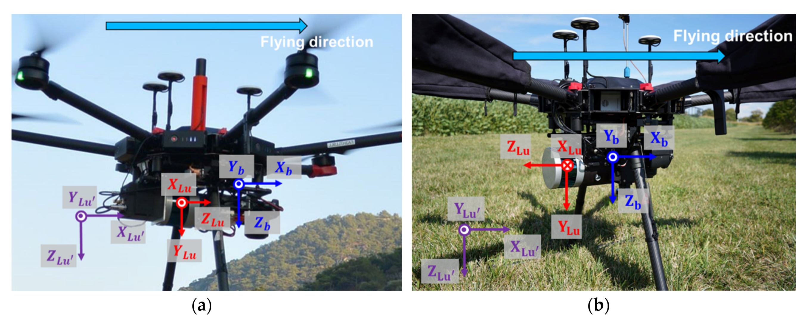
Figure 1.
UAV-based mobile LiDAR mapping systems used in this study: (a) Airborne mobile LiDAR mapping system (MLMS) 1; (b) Airborne MLMS 2.
Figure 1.
UAV-based mobile LiDAR mapping systems used in this study: (a) Airborne mobile LiDAR mapping system (MLMS) 1; (b) Airborne MLMS 2.
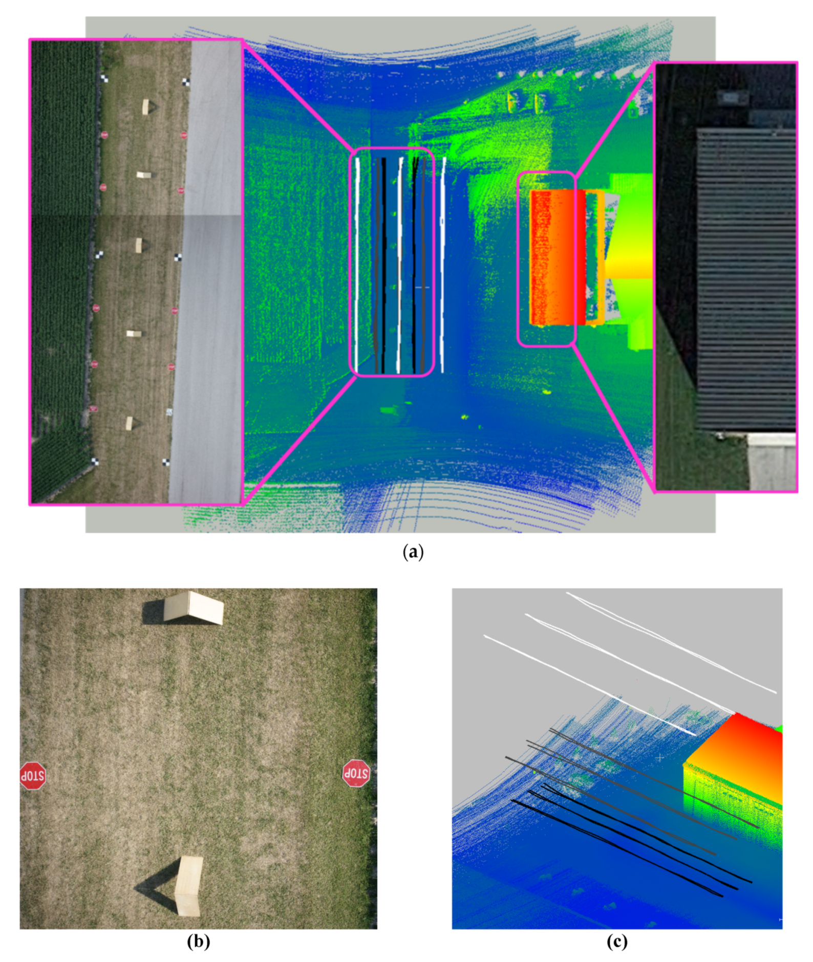
Figure 2.
Calibration test field and flight line configuration for airborne MLMS: (a) 3D point cloud and flight lines colored by height; (b) Close-up RGB image of reflective and hut-shaped targets; (c) Perspective view of flight line configuration colored by height.
Figure 2.
Calibration test field and flight line configuration for airborne MLMS: (a) 3D point cloud and flight lines colored by height; (b) Close-up RGB image of reflective and hut-shaped targets; (c) Perspective view of flight line configuration colored by height.
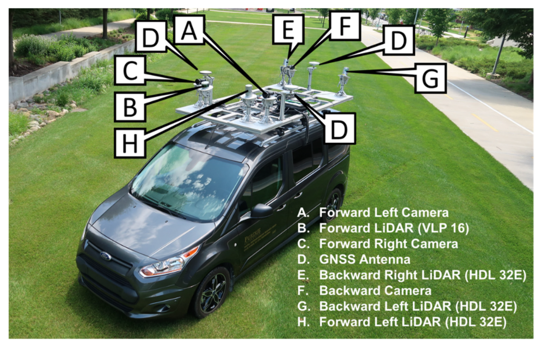
Figure 3.
Terrestrial MLMS used in this study.
Figure 3.
Terrestrial MLMS used in this study.
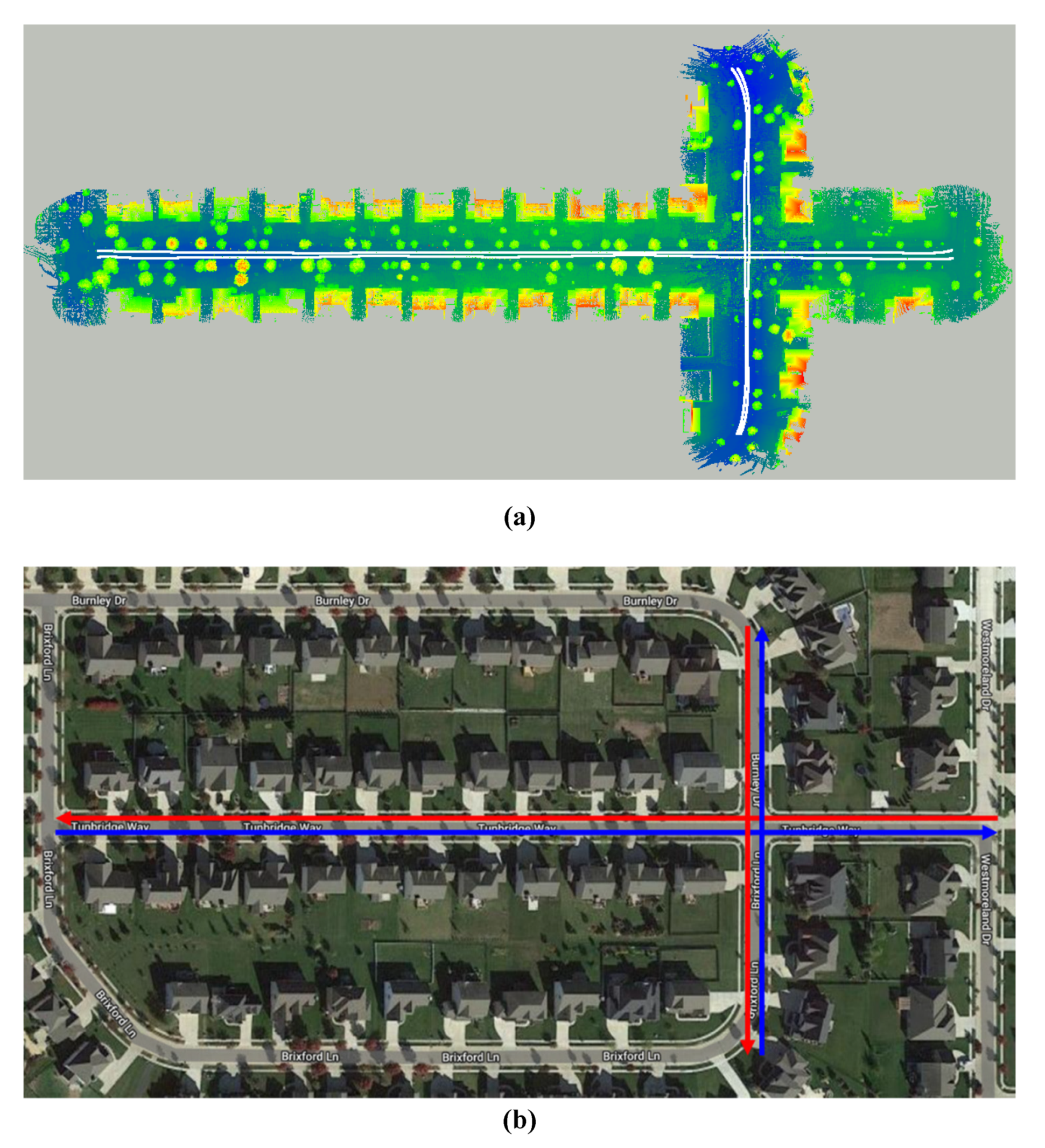
Figure 4.
Calibration test field and drive-run configuration for the terrestrial MLMS: (a) 3D point cloud (colored by height); (b) Satellite view with overlaid drive-runs.
Figure 4.
Calibration test field and drive-run configuration for the terrestrial MLMS: (a) 3D point cloud (colored by height); (b) Satellite view with overlaid drive-runs.
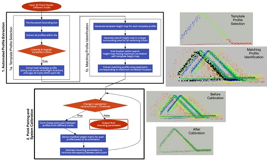
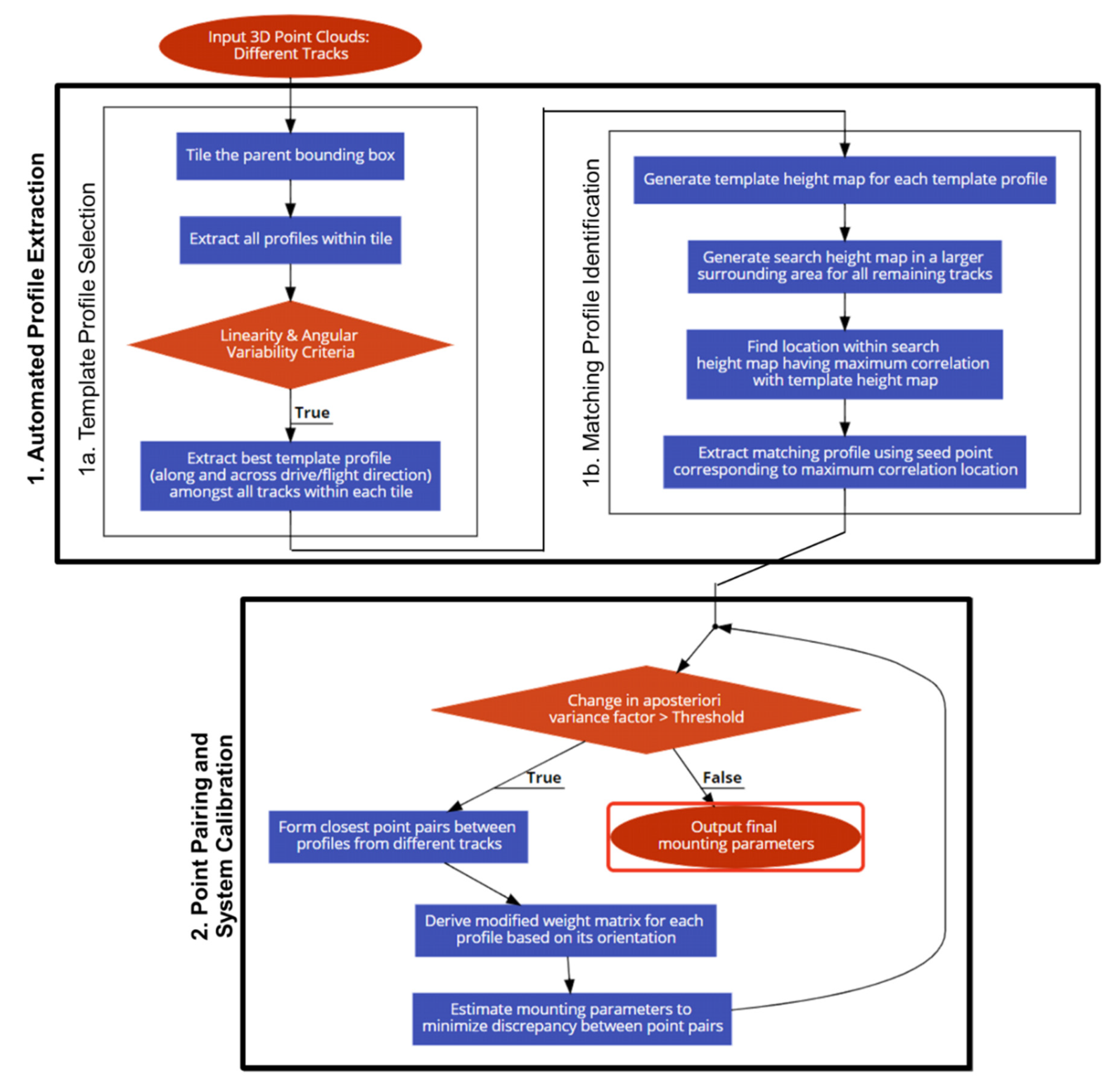
Figure 5.
Flowchart of the proposed profile-based calibration strategy.
Figure 5.
Flowchart of the proposed profile-based calibration strategy.
Figure 6.
Illustration of point positioning for a LiDAR system.
Figure 6.
Illustration of point positioning for a LiDAR system.
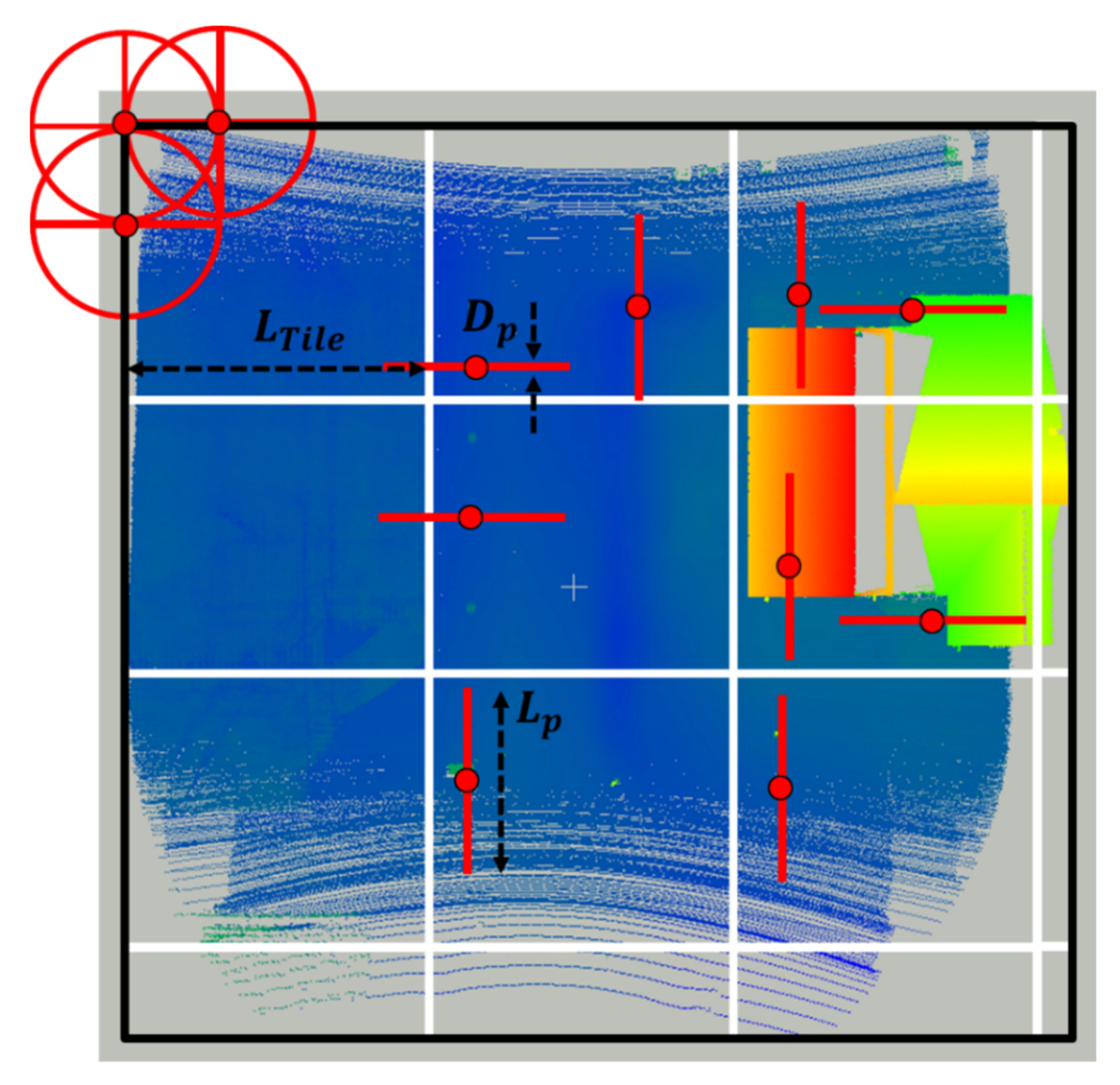
Figure 7.
Illustration of template profile selection for MLMS calibration.
Figure 7.
Illustration of template profile selection for MLMS calibration.
Figure 8.
Illustration of sample profiles with labeled linear (red) and non-linear (blue) points: (a) Retained profile after linearity criterion; (b) Rejected profile after linearity criterion.
Figure 8.
Illustration of sample profiles with labeled linear (red) and non-linear (blue) points: (a) Retained profile after linearity criterion; (b) Rejected profile after linearity criterion.
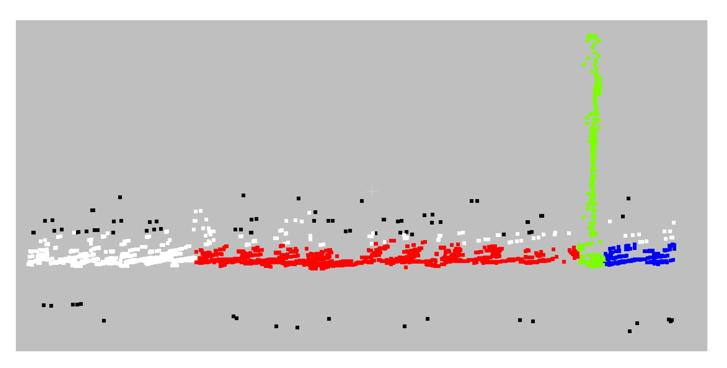
Figure 9.
Sample profile with classified non-linear points (black), linear unsegmented points (white), and three individual line segments (blue, green, and red).
Figure 9.
Sample profile with classified non-linear points (black), linear unsegmented points (white), and three individual line segments (blue, green, and red).
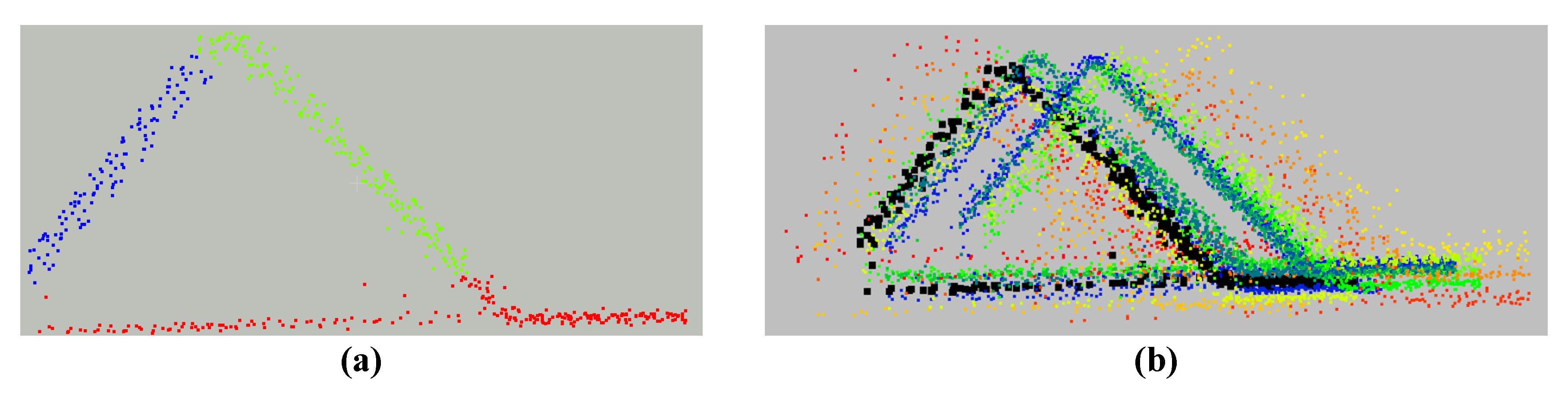
Figure 10.
Sample template and matched profiles: (a) template profile colored by individual fitted lines; (b) same template profile (in black) and its matched profiles in 17 non-reference tracks (colored from blue to red).
Figure 10.
Sample template and matched profiles: (a) template profile colored by individual fitted lines; (b) same template profile (in black) and its matched profiles in 17 non-reference tracks (colored from blue to red).
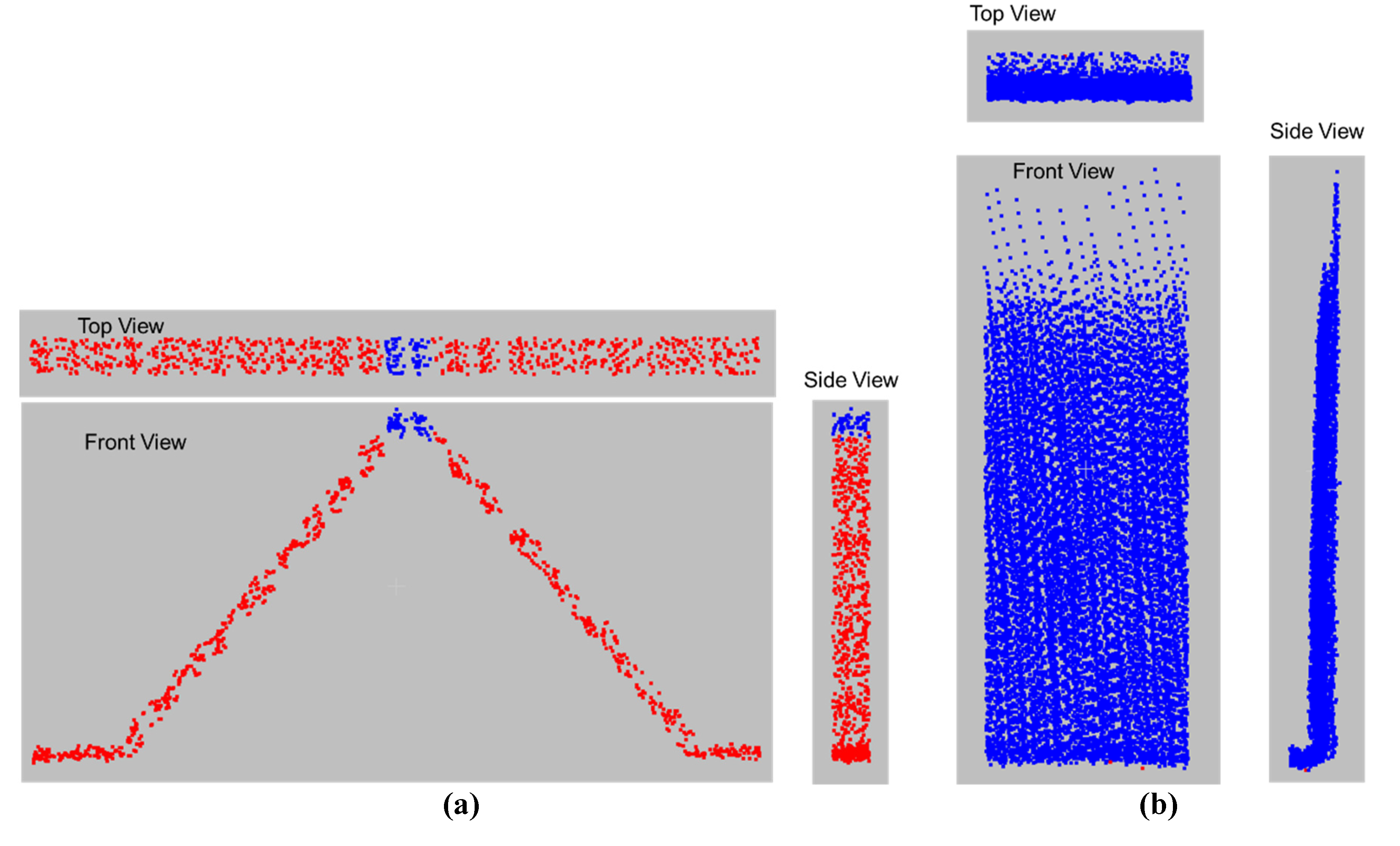
Figure 11.
Sample template and matched profiles along a hut-shaped target: (a) RGB image of hut-shaped target; (b) Top view of template (red) and matched (blue) profiles; (c) Front view of template (red) and matched (blue) profiles.
Figure 11.
Sample template and matched profiles along a hut-shaped target: (a) RGB image of hut-shaped target; (b) Top view of template (red) and matched (blue) profiles; (c) Front view of template (red) and matched (blue) profiles.
Figure 12.
Airborne MLMS 1: template profiles colored by individual line segments.
Figure 12.
Airborne MLMS 1: template profiles colored by individual line segments.
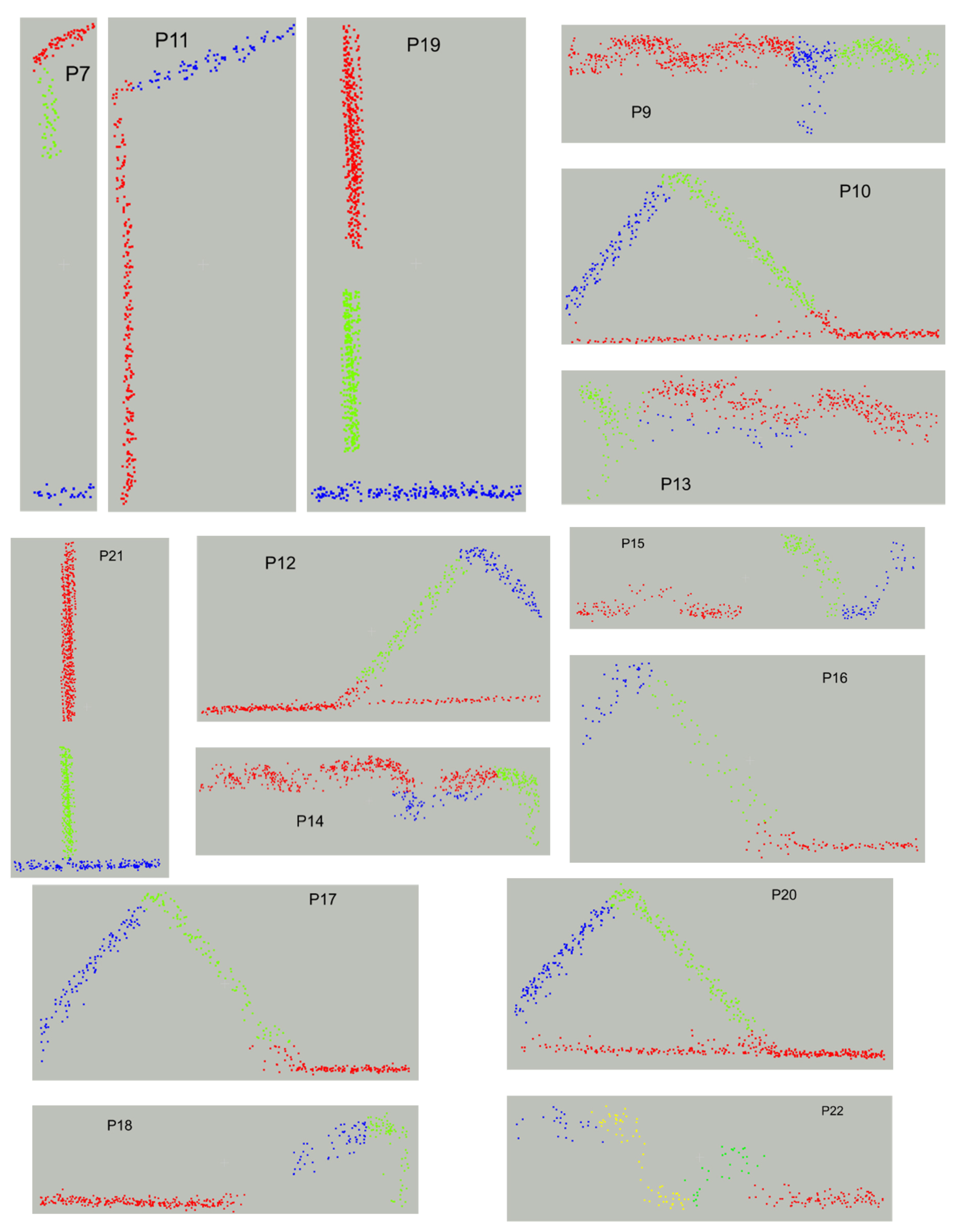
Figure 13.
Airborne MLMS 1: extracted template and matched profiles with profile IDs and reference track number.
Figure 13.
Airborne MLMS 1: extracted template and matched profiles with profile IDs and reference track number.
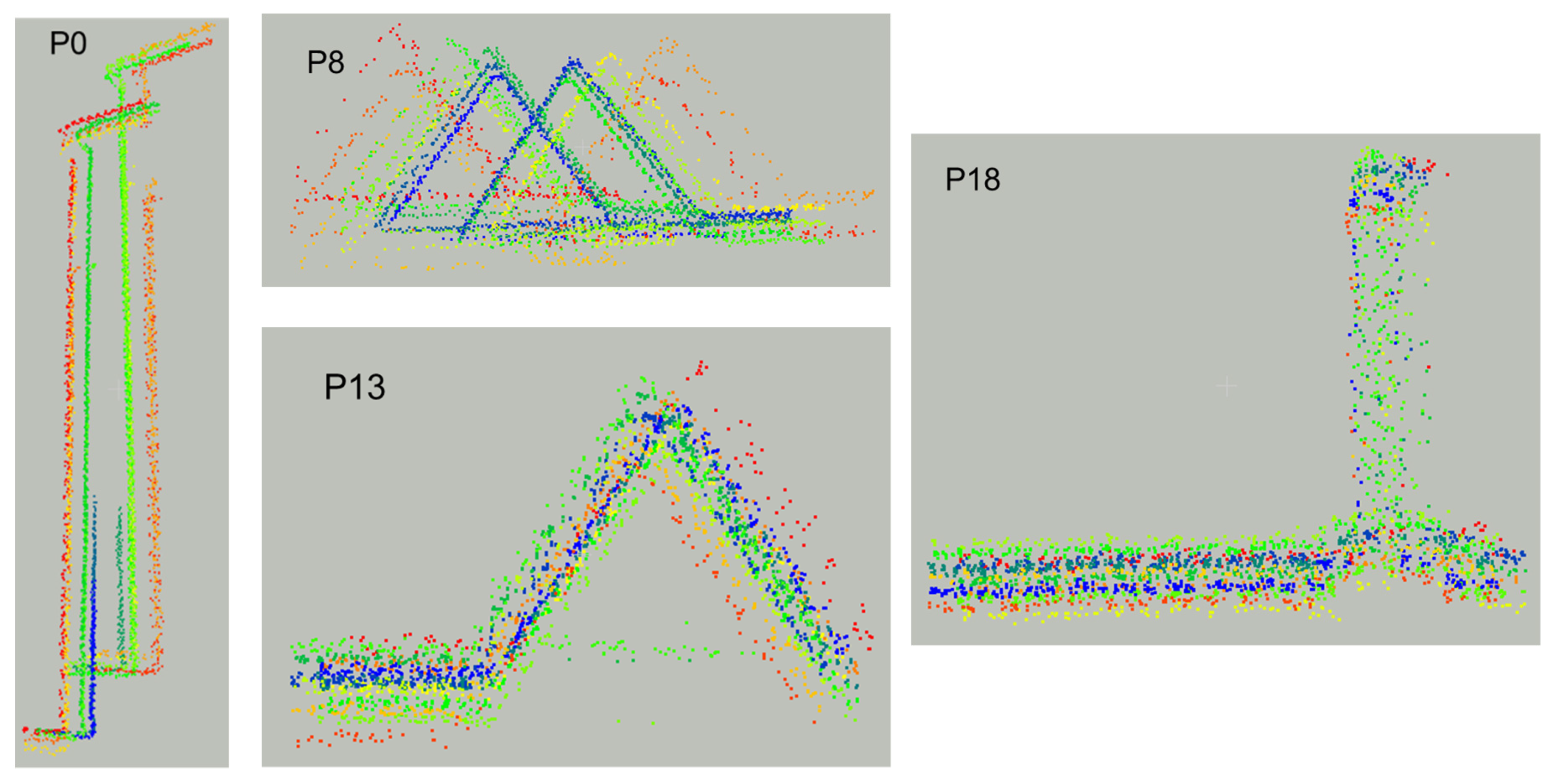
Figure 14.
Airborne MLMS 1: automatically extracted template and matched profiles, where each profile is colored by the track in which it was captured (discrepancy ≈ 2 m).
Figure 14.
Airborne MLMS 1: automatically extracted template and matched profiles, where each profile is colored by the track in which it was captured (discrepancy ≈ 2 m).
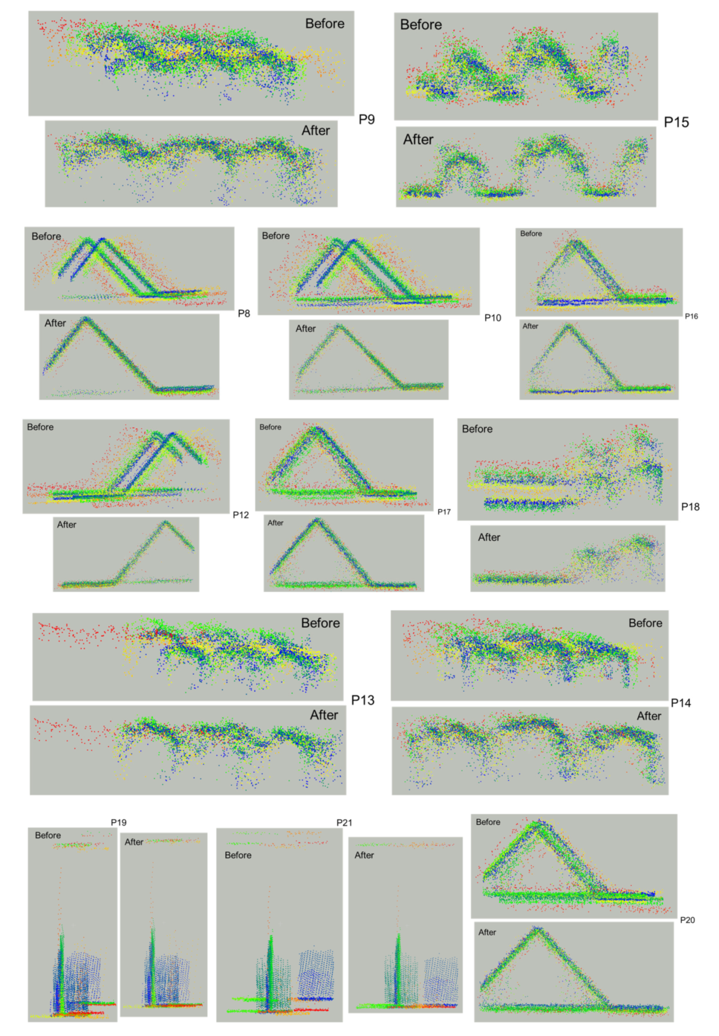
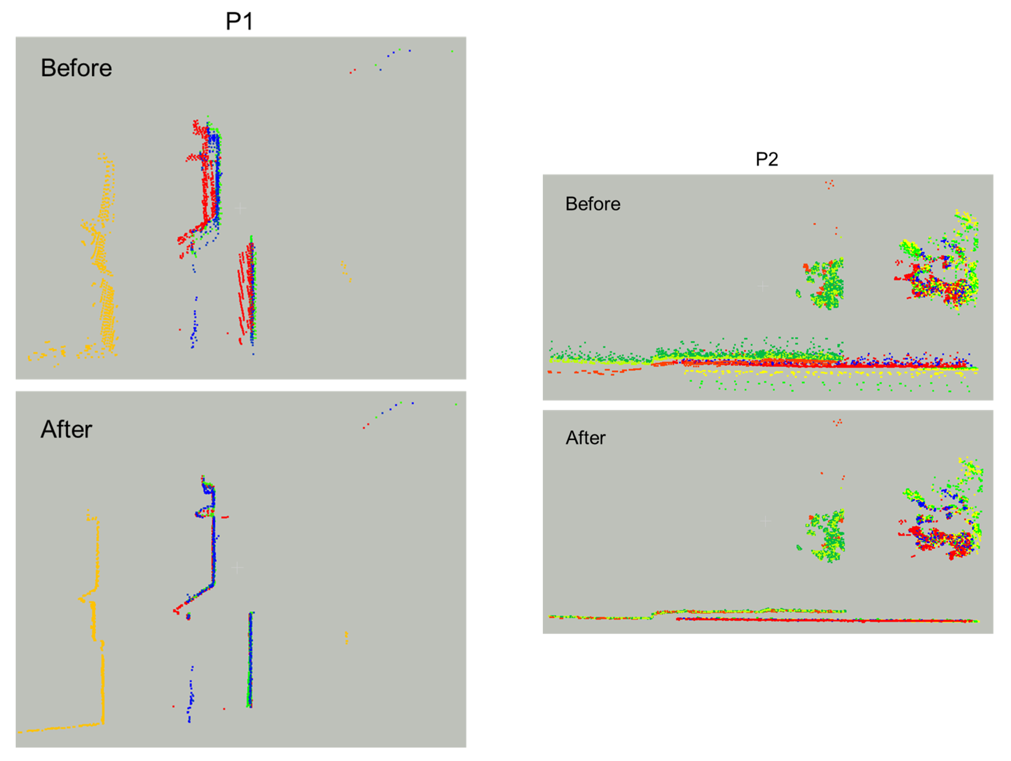
Figure 15.
Airborne MLMS 1: alignment between the profiles (colored by tracks) before and after profile-based calibration .
Figure 15.
Airborne MLMS 1: alignment between the profiles (colored by tracks) before and after profile-based calibration .
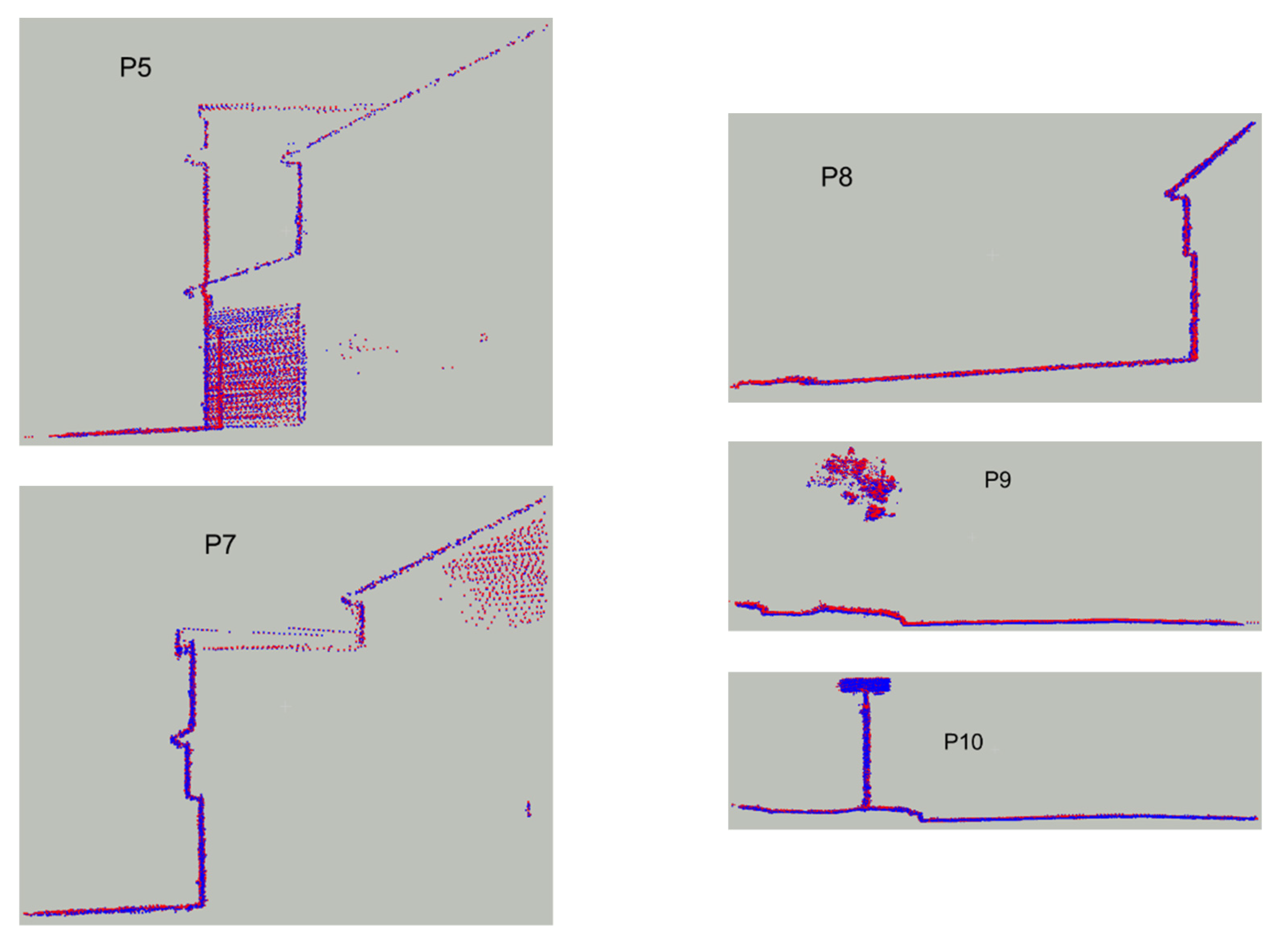
Figure 16.
Airborne MLMS 1: profiles reconstructed from profile-based (blue) and feature-based (red) calibration results.
Figure 16.
Airborne MLMS 1: profiles reconstructed from profile-based (blue) and feature-based (red) calibration results.
Figure 17.
Airborne MLMS 2: sample template profiles colored by individual line segments.
Figure 17.
Airborne MLMS 2: sample template profiles colored by individual line segments.
Figure 18.
Airborne MLMS 2: extracted template and matched profiles with profile IDs and reference track number.
Figure 18.
Airborne MLMS 2: extracted template and matched profiles with profile IDs and reference track number.
Figure 19.
Airborne MLMS 2: automatically extracted template and matched sample profiles, where each profile is colored by the track in which it was captured (discrepancy between tracks ≈ 3 m).
Figure 19.
Airborne MLMS 2: automatically extracted template and matched sample profiles, where each profile is colored by the track in which it was captured (discrepancy between tracks ≈ 3 m).
Figure 20.
Airborne MLMS 2: Alignment between the sample profiles (colored by tracks) before and after profile-based calibration .
Figure 20.
Airborne MLMS 2: Alignment between the sample profiles (colored by tracks) before and after profile-based calibration .
Figure 21.
Airborne MLMS 2: sample profiles reconstructed from profile-based (blue) and feature-based (red) calibration results.
Figure 21.
Airborne MLMS 2: sample profiles reconstructed from profile-based (blue) and feature-based (red) calibration results.
Figure 22.
Terrestrial MLMS: Template profiles colored by individual line segments.
Figure 22.
Terrestrial MLMS: Template profiles colored by individual line segments.
Figure 23.
Terrestrial MLMS: Extracted template and matched profiles with profile IDs and reference track number.
Figure 23.
Terrestrial MLMS: Extracted template and matched profiles with profile IDs and reference track number.
Figure 24.
Terrestrial MLMS: Automatically extracted template and matched sample profiles, where each profile is colored by the track in which it was captured (discrepancy ≈ 1 m).
Figure 24.
Terrestrial MLMS: Automatically extracted template and matched sample profiles, where each profile is colored by the track in which it was captured (discrepancy ≈ 1 m).
Figure 25.
Terrestrial MLMS: Alignment between the profiles (colored by tracks) before and after profile-based calibration .
Figure 25.
Terrestrial MLMS: Alignment between the profiles (colored by tracks) before and after profile-based calibration .
Figure 26.
Terrestrial MLMS: Sample profiles reconstructed from profile-based (blue) and feature-based (red) calibration results.
Figure 26.
Terrestrial MLMS: Sample profiles reconstructed from profile-based (blue) and feature-based (red) calibration results.
Table 1.
Sensor specifications for LiDAR units onboard airborne MLMS: Velodyne VLP32C and VLP16 Puck Lite.
Table 1.
Sensor specifications for LiDAR units onboard airborne MLMS: Velodyne VLP32C and VLP16 Puck Lite.
| | VLP32C | VLP16 Puck Lite |
|---|
| No. of laser beams | 32 | 16 |
| Maximum range | 200 m | 100 m |
| Range accuracy | ±3 cm | ±3 cm |
| Horizontal FOV | 360° | 360° |
| Vertical FOV | 40° (−25° to +15°) | 30° (−15° to +15°) |
| Minimum angular resolution (vertical) | 0.33° | 2.0° |
| Horizontal angular resolution | 0.1° to 0.4° | 0.1° to 0.4° |
| Point capture rate (single return mode) | 600,000 points per second | 300,000 points per second |
Table 2.
Sensor specifications for LiDAR units onboard the terrestrial MLMS: Velodyne HDL32E and VLP16 Puck Hi-Res.
Table 2.
Sensor specifications for LiDAR units onboard the terrestrial MLMS: Velodyne HDL32E and VLP16 Puck Hi-Res.
| | HDL32E | VLP16 Puck Hi-Res |
|---|
| No. of laser beams | 32 | 16 |
| Maximum range | 70 m | 100 m |
| Range accuracy | ± 2 cm | ± 3 cm |
| Horizontal FOV | 360° | 360° |
| Vertical FOV | 41.34° (−30.67° to + 10.67°) | 20° (−10° to +10°) |
| Minimum angular resolution (vertical) | 1.33° | 1.33° |
| Horizontal angular resolution | 0.16° | 0.1° to 0.4° |
| Point capture rate (single return mode) | 700,000 points per second | 300,000 points per second |
Table 3.
Parameters and thresholds used for automated profile extraction.
Table 3.
Parameters and thresholds used for automated profile extraction.
| | Airborne MLMS 1 | Airborne MLMS 2 | Terrestrial MLMS |
|---|
| Template Profile Selection | Tile dimensions | 7 m × 7 m | 20 m × 20 m |
| Profile length | 2 m | 10 m |
| Profile depth | 0.10 m |
| Angular variance threshold | 45° |
| Matching Profile Identification | Height map cell size | 0.20 m × 0.20 m |
| Height map correlation threshold | 90% |
Table 4.
Airborne MLMS 1: angular variation of fitted line segments within selected template profiles.
Table 4.
Airborne MLMS 1: angular variation of fitted line segments within selected template profiles.
| Profile ID | Angular Variance | Profile ID | Angular Variance |
|---|
| P0 | 130° | P12 | 54° |
| P1 | 122° | P13 | 49° |
| P2 | 103° | P14 | 46° |
| P3 | 84° | P15 | 64° |
| P4 | 80° | P16 | 61° |
| P5 | 76° | P17 | 59° |
| P6 | 75° | P18 | 59° |
| P7 | 62° | P19 | 55° |
| P8 | 60° | P20 | 55° |
| P9 | 57° | P21 | 55° |
| P10 | 55° | P22 | 46° |
| P11 | 54° | | |
Table 5.
Airborne MLMS 1: List of tracks (flight lines or sensors) in which each profile was extracted. The track corresponding to template profile is highlighted in yellow
Table 5.
Airborne MLMS 1: List of tracks (flight lines or sensors) in which each profile was extracted. The track corresponding to template profile is highlighted in yellow
| Profile ID | VLP32C |
|---|
| T-1 | T-2 | T-3 | T-4 | T-5 | T-6 | T-7 | T-8 | T-9 | T-10 | T-11 | T-12 | T-13 | T-14 | T-15 | T-16 | T-17 | T-18 |
|---|
| P0 | ✓ | ✓ | ✓ | ✓ | ✓ | | ✓ | ✓ | ✓ | ✓ | | ✓ | ✓ | ✓ | ✓ | ✓ | ✓ | ✓ |
| P1 | ✓ | | ✓ | ✓ | ✓ | ✓ | ✓ | ✓ | ✓ | ✓ | | ✓ | ✓ | ✓ | ✓ | ✓ | ✓ | ✓ |
| P2 | ✓ | ✓ | ✓ | ✓ | ✓ | ✓ | ✓ | ✓ | ✓ | ✓ | | ✓ | ✓ | | ✓ | ✓ | ✓ | ✓ |
| P3 | | ✓ | ✓ | ✓ | ✓ | ✓ | ✓ | ✓ | ✓ | ✓ | | ✓ | ✓ | ✓ | ✓ | ✓ | ✓ | ✓ |
| P4 | ✓ | ✓ | ✓ | ✓ | ✓ | ✓ | ✓ | ✓ | ✓ | ✓ | ✓ | ✓ | ✓ | ✓ | ✓ | ✓ | ✓ | ✓ |
| P5 | ✓ | ✓ | ✓ | ✓ | ✓ | ✓ | ✓ | ✓ | ✓ | ✓ | ✓ | ✓ | ✓ | ✓ | ✓ | ✓ | | ✓ |
| P6 | ✓ | ✓ | ✓ | ✓ | ✓ | ✓ | ✓ | | ✓ | ✓ | ✓ | ✓ | ✓ | | ✓ | | | |
| P7 | | | | | | | ✓ | ✓ | ✓ | | | | | | | | ✓ | ✓ |
| P8 | ✓ | ✓ | ✓ | ✓ | ✓ | ✓ | ✓ | ✓ | ✓ | ✓ | ✓ | ✓ | ✓ | ✓ | ✓ | ✓ | ✓ | |
| P9 | ✓ | ✓ | ✓ | ✓ | ✓ | ✓ | ✓ | ✓ | ✓ | ✓ | ✓ | ✓ | ✓ | ✓ | ✓ | ✓ | | ✓ |
| P10 | ✓ | ✓ | ✓ | ✓ | ✓ | ✓ | ✓ | ✓ | ✓ | ✓ | ✓ | ✓ | ✓ | ✓ | ✓ | ✓ | ✓ | ✓ |
| P11 | | | | | | | ✓ | ✓ | | | | | | | | | ✓ | ✓ |
| P12 | ✓ | ✓ | ✓ | ✓ | ✓ | ✓ | ✓ | ✓ | ✓ | ✓ | ✓ | ✓ | ✓ | ✓ | ✓ | ✓ | ✓ | ✓ |
| P13 | ✓ | ✓ | ✓ | ✓ | ✓ | ✓ | ✓ | ✓ | ✓ | ✓ | ✓ | ✓ | | | | ✓ | | |
| P14 | ✓ | ✓ | ✓ | ✓ | ✓ | ✓ | ✓ | ✓ | ✓ | ✓ | ✓ | ✓ | ✓ | ✓ | | ✓ | ✓ | ✓ |
| P15 | ✓ | ✓ | ✓ | ✓ | ✓ | ✓ | ✓ | ✓ | ✓ | ✓ | ✓ | ✓ | ✓ | ✓ | ✓ | ✓ | ✓ | ✓ |
| P16 | ✓ | ✓ | ✓ | ✓ | ✓ | ✓ | ✓ | ✓ | ✓ | ✓ | ✓ | ✓ | ✓ | ✓ | ✓ | ✓ | | ✓ |
| P17 | ✓ | ✓ | ✓ | ✓ | ✓ | ✓ | ✓ | ✓ | ✓ | ✓ | ✓ | ✓ | ✓ | ✓ | ✓ | ✓ | ✓ | ✓ |
| P18 | ✓ | ✓ | ✓ | ✓ | ✓ | ✓ | ✓ | ✓ | ✓ | ✓ | ✓ | ✓ | ✓ | ✓ | ✓ | ✓ | | ✓ |
| P19 | | ✓ | ✓ | ✓ | | ✓ | ✓ | ✓ | | ✓ | | ✓ | | ✓ | | ✓ | ✓ | ✓ |
| P20 | ✓ | ✓ | ✓ | ✓ | ✓ | ✓ | ✓ | ✓ | ✓ | ✓ | ✓ | ✓ | ✓ | | ✓ | | ✓ | ✓ |
| P21 | ✓ | ✓ | ✓ | ✓ | | ✓ | ✓ | ✓ | ✓ | | | | | ✓ | ✓ | ✓ | | ✓ |
| P22 | ✓ | ✓ | ✓ | ✓ | | | | | ✓ | ✓ | ✓ | ✓ | ✓ | ✓ | ✓ | | | |
Table 6.
Parameters and thresholds used for automated profile extraction.
Table 6.
Parameters and thresholds used for automated profile extraction.
| VLP32C | | | | | | | |
|---|
| Initial Approx. | | 0.06 | 0.03 | 0 | −1 | 0 | 0 |
| Profile-based | Parameters | 0.0177 | 0.0308 | 0.0210 | 0 | −1.5702 | −0.1428 | 0.2371 |
| Std. Dev. | ±0.0105 | ±0.0076 | Fixed | ±0.0102 | ±0.0168 | ±0.0233 |
| Feature-based | Parameters | 0.0220 | 0.0537 | 0.0274 | 0 | −1.5920 | -0.2417 | 0.3372 |
| Std. Dev. | ±0.0122 | ±0.0100 | Fixed | ±0.0135 | ±0.0203 | ±0.0290 |
Table 7.
Airborne MLMS 1: comparison between mapping frame coordinates of profile points derived using profile-based and feature-based calibration parameters (No. of points = 203,163).
Table 7.
Airborne MLMS 1: comparison between mapping frame coordinates of profile points derived using profile-based and feature-based calibration parameters (No. of points = 203,163).
| | | | |
|---|
| Mean | −0.0022 | 0.0213 | −0.0023 |
| Std. Dev. | 0.0180 | 0.0512 | 0.0146 |
| RMSE | 0.0181 | 0.0554 | 0.0148 |
Table 8.
Airborne MLMS 2: angular variation of fitted line segments within selected template profiles.
Table 8.
Airborne MLMS 2: angular variation of fitted line segments within selected template profiles.
| Profile ID | Angular Variance | Profile ID | Angular Variance |
|---|
| P0 | 144° | P10 | 59° |
| P1 | 125° | P11 | 56° |
| P2 | 121° | P12 | 65° |
| P3 | 116° | P13 | 64° |
| P4 | 111° | P14 | 61° |
| P5 | 89° | P15 | 61° |
| P6 | 72° | P16 | 55° |
| P7 | 66° | P17 | 50° |
| P8 | 63° | P18 | 45° |
| P9 | 60° | | |
Table 9.
Airborne MLMS 2: list of tracks (flight lines or sensors) in which each profile has been extracted. The track corresponding to the template profile highlighted in yellow.
Table 9.
Airborne MLMS 2: list of tracks (flight lines or sensors) in which each profile has been extracted. The track corresponding to the template profile highlighted in yellow.
| Profile ID | VLP16 Puck Lite |
|---|
| T-1 | T-2 | T-3 | T-4 | T-5 | T-6 | T-7 | T-8 | T-9 | T-10 | T-11 | T-12 | T-13 | T-14 | T-15 | T-16 | T-17 | T-18 |
|---|
| P0 | | | ✓ | ✓ | ✓ | ✓ | ✓ | ✓ | ✓ | ✓ | ✓ | ✓ | ✓ | ✓ | ✓ | ✓ | ✓ | |
| P1 | | | ✓ | | ✓ | ✓ | ✓ | ✓ | ✓ | ✓ | ✓ | ✓ | ✓ | ✓ | ✓ | ✓ | ✓ | |
| P2 | | | ✓ | ✓ | ✓ | ✓ | ✓ | ✓ | ✓ | ✓ | ✓ | ✓ | ✓ | ✓ | ✓ | ✓ | ✓ | ✓ |
| P3 | | | ✓ | ✓ | ✓ | ✓ | ✓ | ✓ | ✓ | ✓ | ✓ | ✓ | ✓ | ✓ | ✓ | ✓ | ✓ | ✓ |
| P4 | | | ✓ | ✓ | ✓ | ✓ | ✓ | ✓ | ✓ | ✓ | ✓ | ✓ | ✓ | | ✓ | ✓ | ✓ | |
| P5 | ✓ | | ✓ | ✓ | ✓ | ✓ | ✓ | ✓ | ✓ | ✓ | | | | | | | | |
| P6 | ✓ | ✓ | ✓ | ✓ | ✓ | ✓ | ✓ | ✓ | ✓ | ✓ | ✓ | ✓ | ✓ | | ✓ | ✓ | | |
| P7 | | | | | | | ✓ | ✓ | | | | | | | ✓ | | ✓ | ✓ |
| P8 | ✓ | ✓ | ✓ | ✓ | ✓ | ✓ | ✓ | ✓ | ✓ | ✓ | ✓ | ✓ | ✓ | ✓ | ✓ | ✓ | ✓ | |
| P9 | ✓ | ✓ | ✓ | ✓ | ✓ | ✓ | ✓ | ✓ | ✓ | ✓ | ✓ | ✓ | ✓ | | ✓ | | ✓ | |
| P10 | ✓ | ✓ | ✓ | ✓ | ✓ | ✓ | ✓ | ✓ | ✓ | ✓ | ✓ | ✓ | ✓ | | ✓ | | ✓ | |
| P11 | ✓ | ✓ | ✓ | ✓ | ✓ | ✓ | ✓ | ✓ | ✓ | ✓ | | ✓ | | | | | | |
| P12 | | ✓ | ✓ | ✓ | ✓ | ✓ | ✓ | ✓ | ✓ | ✓ | ✓ | ✓ | | | ✓ | | ✓ | |
| P13 | | ✓ | ✓ | ✓ | ✓ | ✓ | ✓ | ✓ | ✓ | ✓ | ✓ | ✓ | ✓ | ✓ | | | | |
| P14 | ✓ | ✓ | ✓ | ✓ | ✓ | ✓ | ✓ | ✓ | ✓ | ✓ | ✓ | ✓ | | | ✓ | ✓ | ✓ | ✓ |
| P15 | ✓ | ✓ | ✓ | ✓ | ✓ | ✓ | ✓ | ✓ | ✓ | ✓ | ✓ | ✓ | | | ✓ | ✓ | ✓ | ✓ |
| P16 | ✓ | ✓ | ✓ | ✓ | ✓ | ✓ | ✓ | ✓ | ✓ | ✓ | ✓ | ✓ | | | ✓ | ✓ | ✓ | |
| P17 | ✓ | ✓ | ✓ | ✓ | ✓ | ✓ | ✓ | ✓ | ✓ | ✓ | ✓ | ✓ | ✓ | ✓ | ✓ | ✓ | ✓ | |
| P18 | ✓ | ✓ | ✓ | ✓ | ✓ | ✓ | ✓ | ✓ | ✓ | ✓ | ✓ | ✓ | | | | | | |
Table 10.
Airborne MLMS 2: manually measured initial approximations, profile-based calibration results, feature-based calibration results, and standard deviation of estimates for the mounting parameters for all the sensors.
Table 10.
Airborne MLMS 2: manually measured initial approximations, profile-based calibration results, feature-based calibration results, and standard deviation of estimates for the mounting parameters for all the sensors.
| VLP16 Puck Lite | | | | | | | |
|---|
| Initial Approx. | | −0.15 | 0.03 | 0 | 0 | 0 | 0 |
| Profile-based | Parameters | 0.0198 | −0.1382 | 0.0263 | 0 | 1.0421 | 0.1130 | −0.0229 |
| Std. Dev. | ±0.0119 | ±0.0092 | Fixed | ±0.0132 | ±0.0206 | ±0.0253 |
| Feature-based | Parameters | 0.0233 | −0.1245 | 0.0478 | 0 | 1.1148 | 0.0746 | −0.0176 |
| Std. Dev. | ±0.0122 | ±0.0079 | Fixed | ±0.0112 | ±0.0196 | ±0.0215 |
Table 11.
Airborne MLMS 2: comparison between mapping frame coordinates of profile points derived using profile-based and feature-based calibration parameters (No. of points = 166,604).
Table 11.
Airborne MLMS 2: comparison between mapping frame coordinates of profile points derived using profile-based and feature-based calibration parameters (No. of points = 166,604).
| | | | |
|---|
| Mean | −0.0006 | 0.0011 | 0.0018 |
| Std. Dev. | 0.0127 | 0.0063 | 0.0291 |
| RMSE | 0.0127 | 0.0064 | 0.0292 |
Table 12.
Terrestrial MLMS: Angular variation of fitted line segments within selected template profiles.
Table 12.
Terrestrial MLMS: Angular variation of fitted line segments within selected template profiles.
| Profile ID | Angular Variance | Profile ID | Angular Variance |
|---|
| P1 | 88° | P7 | 88° |
| P2 | 63° | P8 | 79° |
| P3 | 55° | P9 | 79° |
| P4 | 110° | P10 | 56° |
| P5 | 90° | P11 | 46° |
| P6 | 89° | P15 | 61° |
Table 13.
Terrestrial MLMS: List of tracks (drive-runs or sensors) in which each profile has been extracted. All the tracks in which each profile was identified and extracted with the track corresponding to template profile highlighted in yellow.
Table 13.
Terrestrial MLMS: List of tracks (drive-runs or sensors) in which each profile has been extracted. All the tracks in which each profile was identified and extracted with the track corresponding to template profile highlighted in yellow.
| Profile ID | HDL32E1R | HDL32E2L | HDL32E3F | VLP161F |
|---|
| T-1 | T-2 | T-3 | T-4 | T-1 | T-2 | T-3 | T-4 | T-1 | T-2 | T-3 | T-4 | T-1 | T-2 | T-3 | T-4 |
|---|
| P1 | | | | ✓ | ✓ | | | ✓ | ✓ | | | | ✓ | | | ✓ |
| P2 | | | ✓ | | | ✓ | ✓ | | | ✓ | ✓ | | | ✓ | ✓ | |
| P3 | ✓ | | | ✓ | ✓ | | | ✓ | ✓ | | | ✓ | ✓ | | | ✓’ |
| P4 | | ✓ | ✓ | | | ✓ | ✓ | | | ✓ | ✓ | | | ✓ | ✓ | |
| P5 | | ✓ | ✓ | | | ✓ | ✓ | | | ✓ | ✓ | | | ✓ | ✓ | |
| P6 | | ✓ | ✓ | | | ✓ | ✓ | | | ✓ | ✓ | | | ✓ | ✓ | |
| P7 | | ✓ | ✓ | | | ✓ | ✓ | | | ✓ | ✓ | | | ✓ | ✓ | |
| P8 | | ✓ | ✓ | | | ✓ | ✓ | ✓ | ✓ | ✓ | ✓ | ✓ | ✓ | ✓ | ✓ | ✓ |
| P9 | | ✓ | ✓ | | | ✓ | ✓ | | | ✓ | ✓ | | | ✓ | ✓ | |
| P10 | | ✓ | | | | ✓ | ✓ | | | ✓ | ✓ | | | ✓ | ✓ | |
| P11 | ✓ | | | ✓ | ✓ | | | ✓ | ✓ | | | ✓ | ✓ | | | ✓ |
Table 14.
Terrestrial MLMS: Manually measured initial approximations, profile-based calibration results, feature-based calibration results, and standard deviation of estimates for the mounting parameters for all the sensors.
Table 14.
Terrestrial MLMS: Manually measured initial approximations, profile-based calibration results, feature-based calibration results, and standard deviation of estimates for the mounting parameters for all the sensors.
| HDL32E1R | | | | | | | |
| Initial Approx. | | −1.05 | 0.65 | −0.5657 | 180 | −15 | 0 |
| Profile-based | Parameters | 0.0172 | −1.0517 | 0.6410 | −0.5657 | 180.3183 | −16.7342 | −0.1322 |
| Std. Dev. | ±0.0127 | ±0.0100 | Fixed | ±0.0237 | ±0.0250 | ±0.0268 |
| Feature-based | Parameters | 0.0157 | −1.0567 | 0.6451 | −0.5657 | 180.3146 | −16.7151 | −0.1063 |
| Std. Dev. | ±0.0070 | ±0.0060 | Fixed | ±0.0105 | ±0.0130 | ±0.0118 |
| HDL32E2L | | | | | | | |
| Initial Approx. | | −1.05 | −0.45 | −0.55 | 180 | −18 | 0 |
| Profile-based | Parameters | 0.0172 | −1.0436 | −0.4532 | −0.5615 | 180.1114 | −18.7331 | −0.2844 |
| Std. Dev. | ±0.0125 | ±0.0092 | ±0.0094 | ±0.0234 | ±0.0247 | ±0.0259 |
| Feature-based | Parameters | 0.0157 | −1.0562 | −0.4632 | −0.5638 | 180.1021 | −18.7421 | −0.2645 |
| Std. Dev. | ±0.0065 | ±0.0053 | ±0.0051 | ±0.0100 | ±0.0121 | ±0.0112 |
| HDL32E3F | | | | | | | |
| Initial Approx. | | 1.30 | −0.25 | −0.60 | 180 | 6 | 180 |
| Profile-based | Parameters | 0.0172 | 1.3156 | −0.2703 | −0.5654 | 179.9672 | 7.0761 | 181.0636 |
| Std. Dev. | ±0.0105 | ±0.0089 | ±0.0100 | ±0.0204 | ±0.0202 | ±0.0239 |
| Feature-based | Parameters | 0.0157 | 1.2871 | −0.2727 | −0.5759 | 179.9660 | 7.1094 | 181.0750 |
| Std. Dev. | ±0.0069 | ±0.0057 | ±0.0054 | ±0.0106 | ±0.0123 | ±0.0112 |
| VLP161F | | | | | | | |
| Initial Approx. | | 1.30 | 0.45 | −0.50 | 180 | 10 | -90 |
| Profile-based | Parameters | 0.0172 | 1.3210 | 0.4333 | −0.4915 | 180.0491 | 11.0617 | −90.1805 |
| Std. Dev. | ±0.0181 | ±0.0134 | ±0.0131 | ±0.0279 | ±0.0322 | ±0.0340 |
| Feature-based | Parameters | 0.0157 | 1.3014 | 0.4317 | −0.4887 | 180.0534 | 11.0231 | −90.1349 |
| Std. Dev. | ±0.0087 | ±0.0058 | ±0.0059 | ±0.0117 | ±0.1137 | ±0.0123 |
Table 15.
Terrestrial MLMS: Comparison between mapping frame coordinates of profile points derived using profile-based and feature-based calibration parameters (No. of points = 131,591).
Table 15.
Terrestrial MLMS: Comparison between mapping frame coordinates of profile points derived using profile-based and feature-based calibration parameters (No. of points = 131,591).
| | | | |
|---|
| Mean | −0.0010 | −0.0017 | −0.0040 |
| Std. Dev. | 0.0163 | 0.0128 | 0.0061 |
| RMSE | 0.0163 | 0.0129 | 0.0073 |


