Abstract
In many tropical areas, evapotranspiration is the most important but least known component of the water cycle. An innovative method, named E3S (for EVASPA S-SEBI Sahel), was developed to provide spatially-distributed estimates of daily actual evapotranspiration (ETd) from remote sensing data in the Sahel. This new method combines the strengths of a contextual approach that is used to estimate the evaporative fraction (EF) from surface temperature vs. albedo scatterograms and of an ensemble approach that derives ETd estimates from a weighted average of evapotranspiration estimated from several EF methods. In this work, the two combined approaches were derived from the simplified surface energy balance index (S-SEBI) model and the EVapotranspiration Assessment from SPAce (EVASPA) tool. Main innovative aspects concern (i) ensemble predictions of ETd through the implementation of a dynamic weighting scheme of several evapotranspiration estimations, (ii) epistemic uncertainty of the estimation of ETd from the analysis of the variability of evapotranspiration estimates, and (iii) a new cloud filtering method that significantly improves the detection of cloud edges that negatively affect EF determination. E3S was applied to MODIS/TERRA and AQUA datasets acquired during the 2005–2008 period over the mesoscale AMMA-CATCH (Analyse Multidisciplinaire de la Mousson Africaine—Couplage de l’Atmosphère Tropicale et du Cycle Hydrologique) observatory in South-West Niger. E3S estimates of instantaneous and daily available energy, evaporative fraction, and evapotranspiration were evaluated at a local scale based on two field-monitored plots representing the two main ecosystem types in the area—a millet crop and a fallow savannah bush. In addition to these ground-based observations, the local scale evaluation was performed against continuous simulations by a locally-calibrated soil-vegetation-atmosphere transfer model for the two plots. The RMSE (root mean square error) from this comparison for E3S’s ETd estimates from combined AQUA/TERRA sources was 0.5 mm·day−1, and the determination coefficient was 0.90. E3S significantly improved representation of the evapotranspiration seasonality, compared with a classical implementation of S-SEBI or with the original EVASPA’s non-weighted ensemble scheme. At the mesoscale, ETd estimates were obtained with an average epistemic uncertainty of 0.4 mm·day−1. Comparisons with the reference 0.25°-resolution GLEAM (global land evaporation Amsterdam model) product showed good agreement. These results suggested that E3S could be used to produce reliable continuous regional estimations at a kilometric resolution, consistent with land and water management requirements in the Sahel. Moreover, all these innovations could be easily transposed to other contextual approaches.
1. Introduction
Evapotranspiration (ET), or latent heat flux (LE = λ.ET, where λ is the latent heat of vaporization), is a pivotal surface process that couples the earth’s water and energy cycles. In the tropics, particularly, it plays a major role in surface-atmosphere interactions—a key component of the West African monsoon [1,2] and for vegetation processes. It is strongly related to water stress and to photosynthetic activity, and it is of prime interest to plant productivity management [3]. In typical farm plots of the semiarid West African Sahel, over 80% of the rainwater was estimated to be returned directly to the atmosphere [4], thereby putting a major strain on critical water resources. Yet, ET’s space-time variability and response to environmental changes are still largely poorly captured [5]. This is particularly true in the Sahel [6], where sensitivity to ET of a fast-growing population, relying on rainfed cropping essentially, is very high [7]. Field instruments, such as eddy covariance (EC) systems, are scarce in this area (e.g., the AMMA-CATCH observatory; [8]) and provide only small-scale local estimates, whereas ET may be highly variable in space. The considerable spatial variability in Sahelian rainfall [9] calls for methods, allowing for both large spatial extent and fine resolution. Given its spatial coverage and affordability, remote sensing (RS) in the thermal domain has great potential that remains to be fully harnessed [10]. Over the last two decades, a number of ET estimation techniques, based on remotely sensed land surface temperature (Ts), were proposed with different complexity levels, geographic applicability, and ancillary data requirements. Comprehensive reviews can be found in Kalma et al. [11]; Liou and Kar [12]; Wang and Dickinson [13], and K. Zhang et al. [14]. Among these techniques, the so-called contextual methods, such as the Ts-VI triangle [15,16] and S-SEBI (simplified surface energy balance index; [17]) methods, provide simple ways to derive the evaporative fraction (EF, the ratio of LE to available energy for turbulent fluxes). They are based on cross-scattering of surface temperature and vegetation index (VI) or albedo over a sufficiently flat area with contrasted moisture status. These methods do not require many ancillary data, such as meteorological variables or surface roughness, thereby facilitating their application at the regional scale. As an example, S-SEBI has been applied to a large range of climate conditions and sensors (see e.g., [18,19,20,21,22,23] and Appendix A1); however, to our knowledge, it has never been evaluated in the Sahelian context.
The success of contextual methods in estimating EF and ET mainly depends on the correct determination of the true boundaries of the Ts-VI or Ts-albedo domain [24]. These are the so-called wet and dry edges, corresponding to fully wet or fully dry surfaces, which serve to bound EF values. A variety of algorithms were progressively introduced by S-SEBI or other contextual method users, although rarely fully documented. For the lack of comprehensive and homogeneous evaluation of these techniques, which would require abundant field data in a large variety of situations, no hierarchy can be established between the different algorithms. Hence, they may all be considered as providing a priori equally plausible estimates, suggesting the use of a multi-model approach. Multi-model ensembles have been found to perform significantly better than any single-model in such varied fields as weather and seasonal climate forecast [25,26,27], crop production forecast [28,29], soil moisture simulation [30], or hydrologic prediction [31]. Regarding ET specifically, Ershadi et al. [32] showed that ensemble model estimation was performing better than any individual model in estimating ET across 20 different studied sites. Mueller et al. [33] used a multi-model approach to provide multi-decadal trends in global ET. On the same grounds, the EVASPA (EVapotranspiration Assessment from SPAce; [34]) tool was recently developed to produce ensemble daily ET maps from a combination of several RS-based models (including S-SEBI), RS sources, and edge determination methods [35]. While the ensemble median or mean can be used as the best ET estimate, the range or standard deviation can be considered as expressing the epistemic uncertainty in this estimation. EVASPA was successfully applied over several years to pilot sites in the Crau-Camargue area of Southeast France and in semi-arid areas in Argentina, using MODIS data [34,35,36,37].
When estimating ET over a given area and period, additional information, such as field data, may evidence that all candidate models/methods should not, in fact, be considered as equally reliable estimators. For instance, Garcia et al. [38] evaluated seven edge determination algorithms against ground measurements at two contrasted sites. Rankings differed with type of site and with the season, depending on whether ET was either water- or energy-limited. When considering the multi-model ensemble, such information can be introduced in the estimation procedure through the weighting of ensemble members. Ideally, available observations allow developing a statistical framework to derive weighting coefficients (≥ 0) from the relative performance of each model. For example, Bayesian model averaging (BMA) has been used for continental or global estimation of ET [39,40,41]. However, training BMA against ground observations requires sufficient data to reflect the diversity of situations possibly encountered in the application domain. When these are not available, as in the present case, weighting coefficients may be derived from more empirical approaches that take advantage of background knowledge on processes and model principles. In a situation such as that described by Garcia et al. [38], for instance, weights could be assigned heuristically depending on surface moisture status, seasonal stage, and/or vegetation development, based on each model’s hypotheses and theoretical validity domain. Another difficulty with RS-based ET estimation lies in the frequent uncertainties in key RS variables, such as surface temperature. Contextual methods are considered to be less sensitive to error in Ts than any other method [42,43]. This is true when Ts errors are rather spatially homogeneous due, for example, to sensor calibration or viewing angle. However, it becomes false when Ts errors are due to atmospheric perturbations caused by heterogeneous aerosol content, thin clouds, or cloud edges. A resulting cold Ts bias in contaminated pixels [44] hinders the correct determination of the wet edge. Hence, an additional objective of the E3S (EVASPA S-SEBI Sahel) tool is to further filter MODIS Ts in order to minimize these adverse effects for ET estimation.
In this paper, we proposed an adaptation of EVASPA’s S-SEBI model, denoted as E3S (for EVASPA S-SEBI Sahel), in which edge determination methods were both augmented and time-dependently weighted prior to map daily ET with corresponding epistemic uncertainty. The objective was to substantially improve the estimation of evapotranspiration in the Sahel in comparison to the application of the original S-SEBI contextual method. The new E3S procedure was tested at 1 km-resolution over a 4-year period for an agropastoral Sahelian area of Southwest Niger, using MODIS AQUA and TERRA data. The objectives were to evaluate (i) the potential of the S-SEBI contextual method in the context of the Sahel and (ii) the benefits of the new weighted ensemble scheme compared to a simple mean or to individual members. Among the latter, the Verstraeten et al. [23]’s landmark implementation of S-SEBI (known as the SPLIT method) was singled out as, to our knowledge, it is the only Ts-albedo edge determination algorithm fully described in the literature. The evaluation was performed both at the local pixel scale and over the whole study area (mesoscale, ~104 km2). The local-scale evaluation used EC measurements from two flux towers, as well as reference simulations with the SiSPAT (Simple Soil-Plant-Atmosphere Transfer) detailed land surface model [45], previously calibrated/validated with these measurements [4]. These simulations provided continuous ground-based estimates of available energy—EF and ET—allowing to extend substantially the evaluation. At the mesoscale, E3S was compared with the GLEAM data [46,47], one of the very few spatial ET products with daily availability, and currently, the most recognized for Africa [48], albeit with a lower spatial resolution (0.25°). The benefit of E3S in reducing epistemic uncertainty, compared with the original EVASPA’s S-SEBI method, was also evaluated.
Compared with previous S-SEBI and/or MODIS Ts–based studies, the main novel aspects presented here include:
- (i)
- exploring the potential of the S-SEBI method for the West African Sahel with marked climate seasonality;
- (ii)
- improving the contextual method using an enriched time-variedly weighted ensemble approach and including uncertainty estimation related to wet/dry edges determination;
- (iii)
- enhancing MODIS Ts data for ET estimation through a better assessment of cloud impact.
2. Materials and Methods
2.1. Study Area and Nested Sites
The study area is the 20,800 km2, rectangle meso-site of the AMMA-CATCH observatory in the southwest of the Republic of Niger (1.55°–3.15°E; 12.85–14.15°N; Figure 1a,b), encompassing the capital city of Niamey [8,49]. It is characterized by a tropical semi-arid climate with average annual rainfall decreasing from 570 mm to 470 mm from South to North (1990–2007 average) and a mean temperature of ~30 °C. The West African monsoon brings precipitation within a single wet season from June to September essentially, followed by a long dry season.
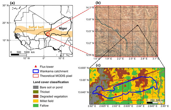
Figure 1.
(a) Location of study area in South West Niger, West Africa; (b) Satellite view of the study mesosite (Google Earth, Image Landsat/Copernicus, image©2017 DigitalGlobe, image©2017 CNES/Airbus); (c) Local-scale Wankama catchment with location of two eddy covariance (EC) flux towers and of corresponding theoretical MODIS pixels, with land cover map derived from a 2005 SPOT image.
The meso-site is crossed in its western part by the Niger River valley and to the east by the large Dallol Bosso fossil valley (Figure 1b). Elevations range from 177 to 274 m above mean sea level. The soils are sandy and poor in nutrients in most of the study area. To the North and East of the Niger River, hydrology is essentially endoreic, whereas the entire South-West bank drains to the river. The main ecosystems are rainfed millet crop and fallow of shrubby savannah, alternating in an agropastoral rotation system. Two single-ecosystem plots in the ~2 km2 Wankama pilot catchment—located in between the two alluvial valleys—were used as local-scale references for the study (Figure 1c). These 15-ha plots have been equipped for EC measurements by the AMMA-CATCH observatory since 2005. During the study period, ecosystems were millet crop and shrubby fallow savannah, respectively. A detailed description of the study area and nested sites can be found in Cappelaere et al. [49].
2.2. Data
2.2.1. Satellite and Other Mesoscale Data
Table 1 describes the 1-km resolution MODIS TERRA and AQUA products used as E3S inputs, for remotely-sensed leaf area index (LAI), normalized difference vegetation index (NDVI), albedo (α), surface temperature (Ts), and emissivity (ε) of land surface (Version 5.5, from the Land Processes Distributed Active Archive Center, https://lpdaac.usgs.gov). Temperature and emissivity were acquired every day at satellite overpass time, but they were subject to many temporal gaps due to cloud cover. To match that resolution, 4-day LAI was daily interpolated by cubic interpolation. The 8-day albedo and 16-day NDVI composites were taken as daytime values over each day within the 8-day or 16-day period.

Table 1.
Description of MODIS data used in this study.
Additional information was required for the E3S method. Rainfall occurrence was obtained from the daily rainfields produced by the AMMA-CATCH observatory from its mesoscale raingauge network [50]. Short and longwave incoming radiations were taken from the ground data at the two Wankama EC stations (next section) and applied uniformly over the mesosite. This upscaling was made possible by the limited spatial variability of incoming radiation under the predominantly clear sky conditions required for image usability. Note that the ground-based information used here could be replaced with alternative sources, such as RS or global or regional modeling. The terrain was described using the DEM GTOPO30 (http://earthexplorer.usgs.gov/). It was used to filter out MODIS pixels based on maximum slope and elevation criteria, albeit with no effect in this study area.
Finally, the global land evaporation Amsterdam model (GLEAM) global ET products were used for mesoscale comparison with E3S results [47]. GLEAM was chosen for this comparison as it is one of the very few RS-ET products available daily and performing well in semi-arid African areas at a regional scale [48]. It is based on a modified Priestley–Taylor formulation with a stress factor based on soil moisture and vegetation water content, coupled with the Gash interception model [51]. In this study, both versions 3.1a and 3.1b were considered [46]. Both versions were available at a native resolution of 0.25° and a daily timestep. They were downloaded in January 2018 from the GLEAM server (https://www.gleam.eu/).
2.2.2. Local Scale Data
The two reference local plots in Wankama are equipped with EC systems, measuring in particular high frequency (20Hz) 3D wind, air temperature, and water vapor, as well as four-component radiation and soil heat flux (Table 2). A full description of all sensors, setup, and other measured variables can be found in Ramier et al. [52] or Velluet et al. [4]. Turbulent fluxes, including ET, were derived as described by Ramier et al. [52], using EdiRe software (R. Clement, University of Edinburgh) and following CarboEurope recommendations [53]. All water and heat fluxes were aggregated to 30-min timestep. Mean energy balance residuals for raw daily daytime fluxes were 3.6 and 14.2 W·m−2 at the fallow and millet sites, respectively [52]. They were attributed, at least, in part to unaccounted-for positive daytime storage in the shallow soil, for lack of shallow soil temperature measurements. EC measurements were not corrected for energy balance closure as residuals were reasonably small and could be attributed to a variety of sources.
Table 2.
Main observations used from the AMMA-CATCH eddy covariance (EC)-stations at Wankama, Niger.
Because these field measurements inevitably included a significant fraction of gaps in the various time series, using the datasets directly for comparison with the RS-based estimates had limitations. This was especially true for daily-integrated fluxes because of the high dependency of the EC method upon aerologic conditions over the day, which seriously reduced the number of days available for direct comparison. Therefore, to allow for a more complete evaluation, the results of the E3S method were also compared with simulations by the physically-based SiSPAT land surface model over 2005–2008. These simulations might be considered as reliable proxies of the local plots fluxes, as the model was thoroughly calibrated and validated by Velluet et al. [4] against the multi-variable dataset from the two EC plots for the 7 years 2005–2012. The model was shown to perform very well against the observations over the wide range of conditions encountered during those 7 years, whether in the calibration or the validation sub-period. Table 3 displays the model’s skill scores calculated for the present study period (2005–2008), for 30-min net radiation, soil heat, and latent heat fluxes. All these values were highly similar to those obtained for the entire model calibration and validation periods (see Table B1 in Velluet et al. [4]). The excellent performance of the model for the very complete set of water and energy variables supported its use as a trustworthy extrapolator of field data for E3S evaluation. Further, the model was suggested as providing a reliable alternative to measurement correction techniques (such as energy balance closure enforcement), or estimation of non-directly measured variables, such as evaporative fraction and surface soil heat flux (at zero depth). Model outputs were also aggregated to the 30-min timestep. While both field-measured and modeled net radiation and evapotranspiration were used for E3S evaluation at satellite overpass, only model outputs were used for day-integrated fluxes.
Table 3.
Skill scores—bias, root mean square error (RMSE), and correlation coefficient (R) of SiSPAT-modeled 30-min net radiation (Rn), soil heat flux at 5-cm depth (G5cm), and latent heat flux (LE), against field observations for this study period (2005–2008) and the two Wankama plots.
2.3. The S-SEBI Method
The S-SEBI model [17] was developed to solve the surface energy balance from RS data. Neglecting canopy storage, the instantaneous energy balance equation, at satellite overpass, could be written as:
where Rn is the net radiation, G the surface soil heat flux, H the sensible heat flux, and LE the latent heat flux (all in W·m−2).
In ordinary daytime situations (e.g., no rain, no oasis effect), H and LE are positive (upward flux) or nil. This and Equation (1) imply that the evaporative fraction EF (-), defined as LE relative to available energy Rn-G (Equation (2)), varies between 0 and 1 from very dry to very wet soil conditions [54].
In the S-SEBI method, LE is derived from Equation (2) by estimating Rn, G, and EF from RS data, given this above property for EF.
Rn is calculated from the radiation balance for incoming and outgoing radiation at the satellite overpass time:
where α is the surface albedo, Ts is the surface temperature, ε is the emissivity, σ = 5.67 × 10⁻⁸ W·m−2·K−4 is the Steffan–Boltzmann constant, and Rg and Ra are the incoming shortwave and longwave radiation, respectively. Used for the derivation of instantaneous but not daily ET, the instantaneous soil heat flux was approximated with an empirical relationship to Rn and the NDVI [55]:
EF was derived from surface temperature Ts and surface albedo α. For each pixel “i” of a satellite scene associated with a given αi albedo value and Tsi surface temperature value, EF was assumed to vary linearly with Ts between two extreme temperatures Tsdry and Tswet, corresponding to dry (EF = 0) and wet (EF = 1) areas respectively (Figure 2):

Figure 2.
Principles of S-SEBI representation of the relationship between surface albedo, surface temperature, and an evaporative fraction (adapted from Roerink et al. [17]).
Tsdry(αi) and Tswet(αi) were inferred from the upper and lower edges of the scatterplot in the (α, Ts) space for that scene, denoted as dry and wet edges, by assuming linear relationships to αi (Figure 2):
where adry, awet, bdry, and bwet are the linear fitting coefficients.
For a given scatterplot, however, there are many different ways of setting these linear edges, yielding as many different implementations of the S-SEBI method.
Note that application of the S-SEBI method is based on three main assumptions: (i) uniformity of atmospheric conditions over each image; (ii) any variation in surface temperature for a given albedo is related to surface water status; (iii) simultaneous presence of a large range of wet and dry areas in each image. In comparison with other evapotranspiration mapping approaches, such as SEBAL [56] or its derivative METRIC [57], S-SEBI does not account for variations in aerodynamic behavior driven by roughness length, wind speed, and air temperature (in relation to the two first hypotheses).
2.4. Implementation in the EVASPA Tool and Adaptation to the Sahel Context: EVASPA S-SEBI Sahel (E3S)
The S-SEBI method is implemented in the EVASPA tool among several RS-based ET estimation methods. EVASPA was developed by Gallego Elvira et al. [34] and Olioso et al. [35] for continuous estimation of daily ET from RS data in the visible and thermal infrared spectral domains, for hydrological and agronomical applications. It was designed for computing an ensemble estimation of ET with an associated uncertainty from the combination of several surface energy balance models and input data from different space sensors. MODIS products were the first ones to be used as inputs in EVASPA, for models based on the derivation of the evaporative fraction from the combination of either albedo and surface temperature (as done in S-SEBI) or of NDVI or vegetation cover fraction and surface temperature (as done in the triangle approach). For each model, several methods for deriving the wet and dry edges have been implemented, and additional methods could be easily included in the EVASPA ensemble.
In this study, only S-SEBI was considered. To improve estimations in the Sahelian conditions, two significant modifications were introduced in the EVASPA processing. The first one concerns the handling of the wet and dry edge determination algorithms (Section 2.4.1): in the new E3S version, twelve additional algorithms were included for a total of seventeen (Appendix A2), and prior ensemble member weighting was introduced. This weighting was set to depend on the stage in the seasonal cycle (Section 2.4.1). The second modification was the introduction of a cloud edge filtering step in the processing chain, to avoid outlier pixels that could distort the Ts-α scatterplot shape (Section 2.4.2). Additionally, a field-calibrated relationship was established to allow for flux upscaling from instant to day values (Section 2.4.3), as proposed by EVASPA. Figure 3 displays a comprehensive flowchart of E3S, showing the main processing steps, with MODIS input data used. In this study, all input variables required by E3S were taken from RS data except incoming radiation and rainfall fields, which were ground-based (Section 2.2.2).
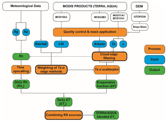
Figure 3.
Flowchart of the E3S (EVASPA S-SEBI Sahel) method. Processes indicated in bold highlight the main modifications brought by E3S compared to EVapotranspiration Assessment from SPAce (EVASPA).
2.4.1. Ensemble Enrichment and Weighting of Edges Determination Methods
A major assumption of the S-SEBI method is that at any time of year, sufficient fully wet and dry pixels would coexist in the same image to allow for the correct determination of the true wet and dry edges. Because of the strong seasonal contrast in the Sahel climate, only one of the two edges can generally be correctly identified, namely the dry edge during the dry season and the wet edge during the wet season. For lack of sufficient informative pixels, application of the standard edge determination algorithms generally leads to a too high wet edge in the dry season and to a too low dry edge in the wet season (denoted as “observed wet edge” and “observed dry edge” in Figure 4a,b, respectively), through undue removal of seeming outliers. Only during the short transition between the wet season and the next dry season, the two extreme conditions coexist in sufficient numbers to allow for reliable determination of both limits with the existing algorithms (Figure 4c). To improve edge determination during the dry or the wet season, new sets of algorithms were introduced, denoted as “dry” and “wet” methods, respectively. “Dry methods” associate the standard dry edge determination algorithms with a simplified wet edge definition consisting of a constant Tswet equal to the absolute minimum observed Ts in the domain (denoted as “observed Tsmin” in Figure 4a). Similarly, “wet methods” associate the standard wet edge algorithms with a constant Tsdry equal to the absolute maximum observed Ts for dry edge definition (denoted as “observed Tsmax” in Figure 4b). Initial methods with the existing standard wet and dry edge determination algorithms are called “transition methods”. Appendix A2 details the list of 17 edge determination algorithms used in this study. Note that despite this large number, this set does not strictly cover all existing methods in the current literature (e.g., [58]).
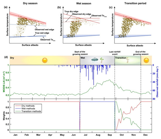
Figure 4.
Typical configurations of the Ts-α scatterplot during (a) the dry season, (b) the wet season, and (c) the transition period. (d) Partitioning of the year 2007 into the three periods, based on leaf area index (LAI) and rainfall (top), and variations of weights for the three classes of associated edges determination methods (bottom).
To reflect the varying degree of suitability of the different algorithms with the seasonal stage, a seasonally-variable weighting procedure was applied. Through the dry season, only the six “dry methods” were given a weight of 1, all eleven others having a weight of 0 (Figure 4d). Conversely, during the wet season, a weight of 1 was assigned to the five “wet methods”, and the twelve other methods being assigned a weight of 0 (Figure 4d). Whereas the shift from the dry to the wet season could be rather precisely dated to the onset of mesoscale rainfall, the presence of significant water storage in the root zone for several weeks after the last rainfall required to handle specifically the wet-dry transition, until the end of the vegetation cycle. At the beginning of this transition period, the concomitant presence of sufficient wet and dry pixels, due to differences in drying rate between vegetated and bare areas, allowed assigning a weight of 1 to the transition methods. Then, as vegetation gets sparser and wet pixels regress, the weight of the transition methods was gradually lowered based on mesoscale average MODIS LAI (Figure 4d). Symmetrically, the weight of the dry methods was gradually raised from 0 to 1 over the transition period based on the same index, and the wet methods were weighted 0.
Accordingly, E3S best estimates were obtained as weighted averages of ensemble members. To express the associated epistemic uncertainty estimates, the range of ensemble members was used in this study, restricted to those members with non-zero weights only and denoted as “conditional ensemble range”, i.e., Range (ETk | weightk > 0), where k designates the kth member in the ensemble.
2.4.2. Cloud Edge Filtering
The contextual methods require efficient outlier filtering, especially due to clouds. Unidentified cloudy pixels can generate false wet pixels and distort the Ts-albedo scatterplot (see Figure A1a,d in Appendix A3), causing systematic biases in EF estimations. We, thus, developed two levels of cloud edge filtering:
- (i)
- The first level filter was based on the quality flag provided by the MOD11A1 and MYD11A1 Ts products for TERRA and AQUA, respectively. A preliminary study showed that cloud edges often corresponded to pixels flagged with a Ts error higher than 1 K, in agreement with Williamson et al. [44]. Thus, all pixels bordering clouds and associated with a Ts error >1 K were removed (see Figure A1b,e in Appendix A3);
- (ii)
- The first level filter was not always sufficient to eliminate all pixels potentially contaminated by clouds, especially during the dry season (Figure A1b in Appendix A3). A second level filter was thus introduced, extending the first level filter to cloud-bordering pixels with Ts below the first Ts quartile in the entire image (Figure A1c,f in Appendix A3). This quantile level selection was calibrated on all the available images outside the rainy seasons in 2005–2008, and we suggested that this could be site- and climate-specific.
Both filter levels needed to be implemented at a scale larger than the study area since pixels flagged as cloudy could be outside the study area. At least, doubling the size of the study area is advisable. The second level filter was only applied outside the rainy period to avoid underestimating wet-season Ts variability, as it was difficult to differentiate between true wet pixels and cloud contaminated pixels passing the first-level filter. After cloud edge filtering, images with less than 8% of remaining pixels (corresponding roughly to 2400 pixels found necessary for the convergence of all edge methods) were eliminated.
2.4.3. Upscaling from Instantaneous to Day-Integrated Fluxes
From the estimation of instantaneous EF and ET at satellite overpass, EVASPA provides time-integrated evapotranspiration for the corresponding day by assuming conservation of the evaporative fraction over the whole day [59]. Neglecting the ground heat flux relative to net radiation at daily scale, the mean daily evapotranspiration (ETd) was then computed as scaled by the ratio Cdi (-) between mean daily net radiation (Rnd) and instantaneous net radiation at satellite overpass (Rn):
where λ is the latent heat of vaporization (λ = 2.45 MJ.kg−1). The Cdi coefficient varies with the day of the year (DOY) and the solar time at a given location according to Wassenaar et al. [60]:
where a1, a2, and a3 are parameters that depend on geographical location and solar time of satellite acquisition. In this study, these parameters were obtained by calibrating Equation (9) on the net radiation averaged from the two EC sites in Wankama from 20 April 2005 to 1 May 2013. Half-hourly and daily observed radiations were used for Rn and Rnd, respectively. Calibrated values and R2 scores are shown for each half-hour of interest in Appendix A4.
2.4.4. Minimizing Gaps in ETd by Combining RS Sources
In order to increase the number of days with available ETd estimates, the AQUA- and TERRA- based, ensemble space-time ETd distributions were merged into a single, blended ensemble ETd product. When and where both sources were available the same day, the two estimates were simply averaged for each ensemble member. This fusion of sources reduced gaps not only in time but also in space on bi-source days. Ensemble ETd estimates were retrieved at 398 dates from 535 MODIS images, including 99 from AQUA only, 162 from TERRA only, and 137 from both satellites. Time coverage by the blended product was 29%, for an average spatial coverage of 79%.
2.4.5. Evaluation Strategy of E3S Estimates
To compare E3S results with available series at the Wankama field plots, and in order to minimize the problem of footprint discrepancy between satellite pixels and EC footprints, it was decided to compare averages of the two adjacent MODIS pixels containing the flux towers with averages of either the measurements at the two plots or of the SISPAT simulations for the two plots. The rationale behind this choice is discussed in detail in Section 4.1.
As a first step, the benefit of the prior weighting of ensemble members introduced in E3S was evaluated. To do so, the E3S estimation was compared both to the use of a single edge determination algorithm, namely the ensemble member denoted as SPLIT, and to the original unweighted ensemble average of EVASPA, hereafter denoted as “EVASPA S-SEBI”. The SPLIT algorithm of Verstraeten et al. [23] (see Appendix A1) was used as a benchmark method as it is the most fully described method for the determination of the wet and the dry edges in the literature.
Estimations of blended ETd were finally compared with the GLEAM products, which might be considered as a reference ETd product at coarse resolution (0.25°) (Section 2.2.1). To this end, E3S estimations were first upscaled at a 0.25° spatial resolution, considering a minimum threshold of 25% of available MODIS pixels in a GLEAM pixel to perform the upscaling by averaging available pixels. Available upscaled ETd was then compared to the corresponding values from the two latest versions of GLEAM (v3.1a and v3.1b).
3. Results
3.1. Local Scale Analysis
3.1.1. Impact of Edge Determination Approach
Figure 5 compares the values of the evaporative fraction (EF) obtained with the SPLIT algorithm, EVASPA S-SEBI, and E3S to those simulated by the SiSPAT model, as scatterplots for the whole study period (left) and as time series for the year 2008 (right). The single wet and dry edge determination algorithm of SPLIT systematically overestimated EF during the dry season (red dots in Figure 5a,b). This was induced by the difficulty in isolating sufficient wet pixels and, as a consequence, to determine the wet edge of the Ts-α scatterplot (Section 2.4.1). Conversely, underestimated EF was obtained during the wet season (blue dots in Figure 5a,b), reflecting the difficulty of the SPLIT approach to identify sufficient dry pixels during this period to determine the dry edge. During the transition period, although conditions of the application were better fulfilled, SPLIT was not able to provide a more accurate EF estimation. In general, the original EVASPA provided slightly better results than SPLIT, even if large EF overestimation in dry and transition periods and large underestimation in the wet period were still observed. Moreover, the uncertainty generated by the use of the unweighted 17 methods (ensemble range, represented as vertical bars, Figure 5d) was usually very large, close to the full 0–1 EF range in many cases. Such large uncertainties suggested that the two approaches were unsuitable to describe the seasonality of EF in the Sahel context.
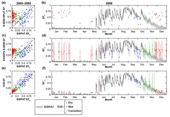
Figure 5.
Evaporative fraction EF estimated with TERRA data by three different edge determination approaches (top to bottom) versus SiSPAT daily EF, for the whole study period (left) and for 2008 (right). (a,b): non-ensemble SPLIT algorithm, Verstraeten et al., 2005; (c,d): original EVASPA S-SEBI unweighted ensemble method; (e,f): E3S weighted ensemble. Uncertainty bars (d,f) correspond to ensemble ranges, conditioned to weighting scheme for E3S (f).
In comparison, E3S provided much better results. The seasonality of EF was well represented, and the weighted mean EF was close to SiSPAT simulations most of the time (Figure 5e,f). Very low EF was observed during the dry season, revealing the efficiency of the newly introduced “dry methods”, with wet edge determination adapted to the lack of wet pixels, in strongly reducing EF overestimation compared with SPLIT and EVASPA. Similarly, E3S significantly reduced EF underestimation in the wet period by the introduction of “wet methods” adapted to the lack of dry pixels. Estimation was also significantly improved during the transition period, showing that the weighted averaging allowed minimizing the impact of seasonally less suitable methods in this period as well. E3S uncertainty, defined as the conditional ensemble range, i.e., the difference between the maximum and the minimum of all those ensemble members whose weight is non-zero (Section 2.4.1.), is shown as vertical bars in Figure 5f. During both the dry and the wet season, uncertainty was considerably reduced, providing much more confidence in the estimation. The uncertainty was still important during the transition period. This was, at least, partly explained by the larger proportion (>2/3) of ensemble members in the conditioned ensemble in that period than in each other period (~1/3), reflecting a larger intrinsic uncertainty (see also discussion in Section 4.3).
The E3S weighted mean of blended ensemble ETd estimates always showed better agreement with the SiSPAT reference than any single ensemble member whatever the period considered. ETd skill scores of each ensemble member are given in Appendix A5, together with those of unweighted (EVASPA) and weighted (E3S) ensemble means. In the rest of this paper, members are no longer considered individually, and the expression “E3S estimates” refers to the weighted ensemble means.
3.1.2. Performance of E3S Estimates over the Study Period
Table 4 displays skill scores of instantaneous and daily fluxes obtained with the new E3S method against both SiSPAT simulations and local plot observations for the 4-year study period, separately for TERRA and AQUA satellite sources. For more detail on E3S performance for daily ET, an analysis of the variations of residual ETd errors (estimated versus SiSPAT-simulated) with the main input variables, is provided in Supplementary Material S1.
Table 4.
Skill scores of E3S (EVASPA S-SEBI Sahel) flux estimates versus SiSPAT simulations or plot observations (when available, in brackets), for instantaneous fluxes at satellite overpass (top five lines) and day-integrated fluxes (last three lines), with TERRA and AQUA satellite sources, over 2005–2008. Determination coefficient (R2) is given without unit whereas Bias and root mean square error (RSME) are given in W·m−2 or in mm·day−1 or without unit according the variable.
Instantaneous Fluxes
In general, the satisfying performance was obtained for instantaneous net radiation estimated with E3S against both ground observations and SiSPAT simulations, at TERRA as at AQUA overpass times. No significant differences were observed between TERRA and AQUA-based estimations, with RMSE (root mean square error) between 35 Wm−2 and 40 Wm−2. A large part of the RMSE was produced by significant positive bias in E3S, in particular for the comparison to ground measurements. This significant Rn overestimation was mainly explained by a negative bias (~−0.01) and relatively high RMSE (~0.02) in MODIS albedo compared to ground observations and SiSPAT simulations from both local plots (not shown). E3S estimations of instantaneous latent heat flux were also in good agreement with observations (Figure 6a,b), with an RMSE value of 43 W·m−2 for AQUA-based estimations. Similar comparisons with SiSPAT simulations showed only very slightly larger values in bias and RMSE (Figure 6c,d), but correlation remained particularly good (R2 of 0.81 and 0.86 for TERRA and AQUA-based estimations, respectively). Better estimation with AQUA, particularly against observations, was mainly due to more underestimation of instantaneous soil heat flux and hence larger overestimation of the available energy at TERRA overpass (bias of 43 W·m−2 in Rn-G). Note that poor correlation was obtained for both TERRA and AQUA-based instantaneous G estimates, showing the limitations of the empirical formulation used in this study.

Figure 6.
Comparing instantaneous latent heat flux (LE) estimated by E3S with plot observations (a,b) and SiSPAT simulations (c,d) at TERRA (a,c) and AQUA (b,d) overpass times.
Evaporative Fraction (EF and EFd)
Instantaneous E3S estimation of EF showed good performance in comparison with SiSPAT-simulated instantaneous EF for the two MODIS satellites (Figure 7a,b), with maximum bias and RMSE of 0.12 and 0.16, respectively, and an R2 of 0.83. No significant differences were obtained between the two satellite sources: both provided an overestimation of instantaneous EF, in relation to the overestimation of LE. The better agreement was observed with daily EFd simulated by SiSPAT (Figure 7d), with a large reduction in this overestimation. This might suggest that the hypothesis of conservation of EF over the daytime might not be fully satisfied (see discussion in Section 4.2, Subsection “Daily fluxes”). This observation was valid whatever the overpass time considered, as a comparison of AQUA and TERRA-based EF estimates (when both were available) showed low bias (−0.02) and RMSE (0.10).

Figure 7.
Comparing evaporative fraction EF estimated by E3S with SiSPAT-simulated instantaneous EF (a,b) and daily EFd (c,d) at TERRA (a,c) and AQUA (b,d) overpass times.
Daily Fluxes
E3S estimations of daily net radiation Rnd (Table 4) were well correlated to SiSPAT simulations (R2 = 0.87), with a slight and similar overestimation for AQUA and TERRA (bias of 6 and 5 W·m−2, respectively), and similar RMSE (13–14 W·m−2). Similar behavior was observed for daily evapotranspiration ETd, with an R2 value of up to 0.89 for the TERRA source (Figure 8). No significant difference in E3S skill scores was obtained between TERRA and AQUA, which was in agreement with results for the other variables used for ETd estimation, namely Rnd and EF. The RMSE of 0.5 mm·day−1 for ETd was equivalent to that for Rnd (converted into water evaporation). RMSE and R2 scores obtained with the AQUA/TERRA blended ETd product against SiSPAT simulations were 0.5 mm·day−1 and 0.90, respectively, with virtually no bias. Quite similar results were obtained when considering each of the two Wankama plots with their corresponding satellite pixel individually (RMSE = 0.5–0.7 mm·day-1, R2 = 0.83–0.87, and absolute bias ≤ 0.1 mm·day-−1). The annual time series of the blended ETd product with its associated epistemic uncertainty is shown in Figure 9 for the period 2005 to 2008. Patterns of variation of ETd errors with albedo, surface temperature, global or atmospheric radiation, and ETd magnitude are described in Supplementary Material S1.
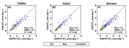
Figure 8.
Daily ETd estimated by E3S from TERRA data (a), AQUA data (b), and combined TERRA/AQUA data (c) versus simulated by SiSPAT.

Figure 9.
E3S blended daily ETd for (a) 2005, (b) 2006, (c) 2007, and (d) 2008 from MODIS combined TERRA-AQUA data versus SiSPAT-simulated ETd. Error bars represent the conditional ensemble range. The shaded grey area represents the variation between the two simulated sites (millet and fallow plots).
3.2. Mesoscale Analysis
3.2.1. E3S Daily ETd
Figure 10a–c shows sample ETd maps produced by E3S (weighted ensemble mean) with the TERRA source over the study meso-site, in the dry season, in the wet season, and the transition period of 2007, respectively. During all dry seasons and for both RS sources, ETd remained very low over most of the study area, with the exception of the Niger River floodplain where ETd remained substantial throughout the year (see, e.g., Figure 10a). Conversely, during the wet seasons and transition periods, patterns of high ETd values were obtained over the whole study area, but never covering its entirety (e.g., Figure 10b,c). Maximum values were observed for the exoreic subarea (right bank of the Niger River) and in the southern part of the left bank of the Niger River, which is characterized by a shrub layer interspersed with bare soil and grass patches. The Dallol Bosso fossil valley, near the east edge of the mesosite, appeared as a dry area whatever the season considered (e.g., Figure 10b), in relation to high albedo values observed in this area. Corresponding albedo and Ts maps are provided in Appendix A6 for broader understanding. A North-South general positive gradient was also observed, especially during the transition period (Figure 10c), which is consistent with the latitudinal gradient of rainfall and vegetation cover fraction (not shown). In the wet season (Figure 10b), the high local-scale variability—with particularly sharp gradients on short distances—over large areas that shift in time, confirmed the need for at least the moderate spatial resolution used in this study.

Figure 10.
Examples of daily ETd maps from E3S with TERRA data (a) on a dry day, 22 January 2007, (b) a wet day, 12 September 2007, and (c) a transition day, 05 October 2007. White pixels mean non-available data.
3.2.2. ETd Uncertainty
For each E3S estimation date, a map of associated uncertainty, defined as the conditional ensemble range, was also produced. Figure 11 displays, for each period of the year, the spatial distribution of temporal mean uncertainty over the study period, for the AQUA/TERRA blended ETd product. It revealed patterns of highest uncertainty for ecosystems associated with the highest ET values, in particular, in the Niger River floodplain, the exoreic subarea on the Niger River’s West bank, and the southern part of the East bank. Largest uncertainty contrasts were obtained in the transition period (Figure 11c).
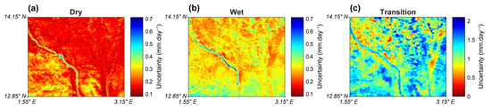
Figure 11.
Spatial distribution of temporal mean uncertainty on E3S daily blended ETd estimates over the study period for (a) the dry season, (b) the wet season, and (c) the transition period. E3S uncertainty is defined as the conditional ensemble range. Please note the different color scale in (c).
Figure 12 displays the distributions of temporal mean uncertainty on ETd as boxplots per period, distinguishing the satellite sources (TERRA, AQUA, and combined TERRA/AQUA). As already reported in Section 3.1.1, uncertainties were significantly greater during the transition period. No significant differences were observed between uncertainties associated with TERRA- and AQUA-based estimates, with only slightly larger values for TERRA during the wet season. Uncertainties on the blended AQUA/TERRA ETd product were logically also very similar to those for the separate sources, with overall means of 0.2 mm·day-1 for the dry season, 0.3 mm·day−1 for the wet season, 1.2 mm·day−1 for the transition period, and 0.4 mm·day−1 for the whole-year period. Uncertainty estimates are discussed in Section 4.3.
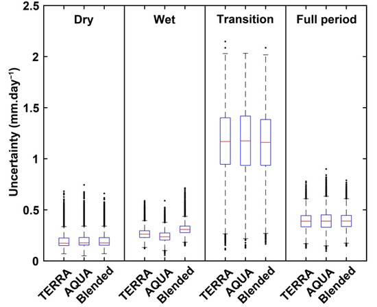
Figure 12.
Boxplots of spatial distributions of temporal mean uncertainty on E3S ETd estimates, for each period of the year (top) and each satellite source (bottom).
3.2.3. Comparing with GLEAM ETd
Figure 13 compares maps of mean seasonal ETd from E3S, GLEAMv3.1a, and GLEAMv3.1b homogenized products (see Section 2.4.5), for the dry season, the wet season, and the transition period. In all three products, spatial patterns were dominated by the regional North-South gradient, whatever the period. Despite the coarse resolution, the presence of the Niger River valley could also be detected, at least, in its northwestern part, in the dry season (Figure 13a,c). During the wet season, spatial variability was quite comparable between upscaled E3S and GLEAMv3.1b, but lower in GLEAMv3.1a. Conversely, upscaled E3S showed substantially lower spatial variability than both GLEAM products during the dry season and the transition period.
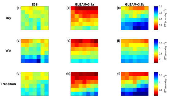
Figure 13.
Maps of mean seasonal ETd at 0.25° resolution, from upscaled E3S (a,d,g), GLEAMv3.1a (b,e,h), and GLEAMv3.1b (c,f,i), for the dry season (a,b,c), the wet season (d,e,f), and the transition period (g,h,i) over 2005–2008. GLEAM: global land evaporation Amsterdam model.
Figure 14 compares the mesoscale-averaged, homogenized E3S, and GLEAM estimations of daily ETd, for all available days in the study. Good agreement was obtained for both GLEAM versions, with R2 higher than 0.90 and RMSE around 0.4 mm·day−1. A slight positive bias of 0.3 mm·day−1 was observed only with the GLEAM version v3.1a. Altogether (Figure 14), E3S appeared to agree particularly well both spatially and temporally with GLEAMv3.1b during the wet season, when evapotranspiration was most important.

Figure 14.
Comparing mesoscale-averaged daily ETd from blended E3S and GLEAM versions (a) 3.1a and (b) 3.1b.
4. Discussion
4.1. Limitations of Satellite-Versus-Field Estimates Comparison
A general difficulty for ground validation of RS products lies in the rarely sufficient availability of reliably-estimated, comparable field variables. Section 2.2.2 explains and justifies why both station data and process model simulations were used here to address this difficulty. In any case and as in any similar study, skill scores have to be interpreted with some caution. Uncertainty in field-measured or even more so, in model-simulated fluxes have to be kept in mind. Discrepancies in footprints between satellite pixels and flux tower footprints, both of which vary over time, may blur the direct comparison of these two sources of flux estimates [61,62]. Given the subkilometric scale of the fields mosaic in the study area (Figure 1b), MODIS pixels could hardly be expected to sample as homogeneous ecosystems as ground stations do. This is all the more true as the contributing area of a MODIS pixel is actually larger than the “theoretical” 1 km2 area, and as its actual position may be somewhat different [63,64]. Hence, rather than comparing directly and separately the estimations for a MODIS pixel, supposedly including a flux station, with those derived from this specific station, it was decided for the comparison to lump estimates from the two stations on one hand and the two corresponding, theoretical MODIS pixels on the other hand, by simple averaging (Section 3.1). The two flux stations sample, respectively, the two main ecosystems (millet crop and shrubby fallow savannah) in the catchment [65] as in the study area. These ecosystems fill most of the surface area covered by the two MODIS pixels, in relatively similar fractions. The sensitivity of this distribution to possible errors in the delineation of these two pixels appears to be rather small. Furthermore, surface response contrasts between cover types are mild enough [4] to dampen possible differences in upscaling performance between averaging schemes of EC stations [66]. Hence, this simple averaging strategy, applied to both the satellite pixels and the EC stations, is expected to minimize possible biases that could arise with respect to lack of colocation or underlying ecosystem similarity in the compared satellite and ground series. Note, however, that E3S estimation performance for daily ETd was essentially conserved when measured individually for each pixel against its corresponding field plot (Section 3.1.2, Subsection Daily fluxes).
4.2. Quality of E3S-Estimated Flux Distributions
To our knowledge, previous applications of the S-SEBI method generally dealt with forests or well-watered croplands in higher latitudes, and this study was the first to test the method in the Sahelian context. In comparison with previous studies, the evaluation was performed over a larger number of dates (~400 days) distributed over a longer period (4 years).
4.2.1. Instantaneous Fluxes
E3S was found to provide acceptable performance for instantaneous net radiation (overall RMSE of 35–40 W·m−2, Table 4), better than usually reported in the literature for RS estimates [67,68,69]. However, direct comparison is difficult as ground data were used here for incoming shortwave and longwave radiation, for which variables generally bring substantial uncertainty to Rn estimation [70]. Using this ground forcing, entailed a loss of spatial variability information relative to satellite-derived inputs, but this loss should be small (Section 2.2.1) and avoid the RS biases. Either source could be used for E3S implementation. The significant overestimation in Rn estimates from both TERRA and AQUA sources was mainly explained by the negative bias (~−1%) in MODIS albedo compared to albedo simulated by SiSPAT, as incoming radiation was the same. Bias and RMSE values estimated here for MODIS albedo (not shown) were similar to those reported for other Sahelian areas [71].
The instantaneous soil heat flux was always poorly estimated (Table 4). Other empirical G formulas, based on vegetation cover fraction [72], LAI [73], or evaporative fraction [74], were tested against SiSPAT simulations, showing a similar performance (not shown). In general, these empirical formulas were calibrated for specific eco-climatic conditions and specific overpass times, causing their lack of transferability. Large differences were observed in G estimates between TERRA and AQUA sources, with opposite bias and quite a good correlation for AQUA. This was due to the phase shift between G and Rn cycles that make the efficiency of empirical parameterizations, such as Equation (4), depend on the overpass time [75].
E3S estimates of evaporative fraction EF showed positive bias (Table 4), occurring in the dry season essentially (Figure 5). In this period, soil moisture is very low in most of the area, except for the irrigated Niger River floodplain (also around ponds, but these areas are not significant within ~1 km2 MODIS pixels), and the wet edge is the most difficult to identify precisely. EF should be predominantly nil or close to, including in the Wankama evaluation pixels; consequently, errors tended mechanically to be generally positive, leading to this bias. However, error magnitudes were comparatively generally low (Figure 5e) because (i) the above few wet pixels, with appropriate EF values of 1 or near to (unstressed conditions, allowing evapotranspiration at potential rate), were relatively informative of wet edge location and (ii) the relative proximity of most pixels to the dry edge (Figure 4a) attenuated EF sensitivity to wet edge determination.
Oppositely, in the wet season, totally dry pixels rarely existed at MODIS resolution, leading to false zero EF values and an imprecise dry edge. Soil moisture and hence dependent Ts being more widely distributed between the two edges (Figure 4b), sensitivity to dry edge determination might be greater than in the dry season, leading to some more significant error magnitudes (Figure 5e). However, there no longer was any determinism on error signs, leading to smaller bias than in the dry season. This also generally applied to the transition period.
RS-based EF estimates are rarely evaluated in the literature, limiting possible comparison with results for similar eco-climatic and sensor conditions. RMSE values obtained here (0.15–0.16, Table 4) were higher than those reported by Verstraeten et al. [23] for European forests (in the ~ 0.06–0.09 range depending on the site, using the S-SEBI approach and the SPLIT edge determination method). Applying S-SEBI with MODIS data to five contrasted sites in India, Eswar et al. [76] reported an RMSE value of 0.14, similar to the one obtained here.
The significant positive bias found in instantaneous latent heat flux (LE, Table 4) was mainly explained by the overestimation of both EF and available energy (Rn-G). Differences between TERRA and AQUA-based estimates (lower bias and RMSE values for AQUA than for TERRA) came from the above-mentioned difference in efficiency on G. RMSE values (43–56 W·m−2) fell in the range reported in the literature with the S-SEBI method (see Appendix A1).
4.2.2. Daily Fluxes
Better evaporative fraction estimates were obtained when upscaling to daily EFd, with both the positive bias and the RMSE being reduced. This behavior should be related to the observation that the upscaling hypothesis of EF daytime invariance was not fully verified in SiSPAT simulation outputs: generally, higher modeled daily EFd than overpass-time EF (not shown, also reported by Delogu et al. [77] or Gentine et al. [78]) was thus less overestimated by E3S. Figure 7 shows that improvements were mainly obtained in the wet season (blue dots) and not in the dry season (red dots). This was in agreement with the reported better daytime conservation of EF in drier situations [77,78,79], water becoming then a stronger constraint than insolation.
Accuracy of Rnd estimates depends in part on the efficiency of the Cdi approximation (Equation (9)). One source of error is the temporal difference between instant Rn and discrete, time-integrated Cdi. A sensitivity analysis showed that accuracy sharply increased with Cdi resolution at times away from noon (RMSE of 14 and 32 W·m−2 for TERRA-based Rnd estimation at half-hourly and hourly resolution, respectively, but little impact on AQUA-based estimation). The Cdi polynomial formulation of [22] was also tested, showing poorer calibration than the sinusoidal formulation of [60] used here. Overall, E3S performance for Rnd was quite satisfying (Table 4), with better correlation (R2 = 0.87) than for Rn, and low RMSE and bias (14 and 6 W·m−2 for TERRA, slightly better for AQUA).
Finally, ETd estimates showed an RMSE value (0.5 mm·day−1; ~14 W·m−2) in the range of values reported in the literature for the S-SEBI method (see Appendix A1). Remarkably, quasi unbiased ETd (Table 4) resulted from the product of both slightly positively biased EFd and Rnd. At the mesoscale, the good agreement of E3S with the reference GLEAM product, together with its much finer spatial resolution, strongly encourages to extend its application to larger scales and to other settings in West Africa.
4.2.3. Benefits of Weighted Ensemble Approach
As documented in Appendix A5 and illustrated by Figure 5a,b, no single edge determination method did as well as E3S for estimation of instantaneous or daily EF or ET. Further, Figure 5c,d highlighted limitations of the unweighted ensemble approach, as the resulting estimate appeared to be strongly biased most of the year and the uncertainty to be quite large (Section 3.1.1). Allocating dynamic weights to ensemble members, depending on method suitability to prevailing conditions, allowed to enhance estimation accuracy and to reduce uncertainty drastically. The seasonal weighting approach proposed in this study always outperformed both non-ensemble and unweighted ensemble approaches, including in transition periods through gradually-varying weights.
Beyond this study case, weighted ensemble RS estimation of ET should be preferred to single estimation as it seems impossible to determine a “best method” for a sufficiently large range of eco-climatic contexts and for most conditions possibly encountered in a given context. We suggested that the seasonal weighting approach introduced here could be transposed to any other climatic region with marked seasonality, for ensemble RS-based ET estimation using any contextual method. It could be easily applied, for instance, with the Ts-VI Triangle method [16]. When possible, weight allocation might be performed through objective statistical techniques, such as BMA (e.g., [40]). However, the frequent lack of ground ET measurements is usually very limiting for the training of such statistical methods over a sufficient range of conditions, especially in data-poor regions like most of the African continent. In this respect, more empirical approaches for assigning weights heuristically according to prior knowledge on methods characteristics and behaviors, as introduced in this study, have great potential.
4.3. Uncertainty
During the dry and wet seasons, estimated uncertainty rarely exceeded E3S error computed from ground estimates (Figure 9). Oppositely, during the transition period, the uncertainty was generally much larger than the error. These observations highlighted the limitations of the current estimation of uncertainty by E3S and underlined that E3S uncertainty, as expressed by the conditional ensemble range, should by no means be interpreted as some sort of confidence interval. Indeed, Ts-α edge determination methods are not the only source of uncertainty in ET estimation, even though they are likely to be one of the largest [24]. Other sources, such as uncertainties in input data or on the degree of satisfaction of the method’s underlying hypotheses, should also be accounted for. For epistemic uncertainty itself, contributions from the other component parameterizations (e.g., Equations (4), (5), (8) and (9)) should also be considered.
Regarding the satisfaction of hypotheses, window choice is an important uncertainty factor for contextual methods [80,81]. This choice must arise from a compromise between conflicting requirements for both meteorological uniformity and sufficient diversity in soil moisture status at all application times. Both are affected oppositely by window size, but the second one depends primarily on landscape configuration, as well as on-sensor spatial resolution. Interactions between these three factors would make it a heavy task to quantify effects on estimation accuracy.
If one sticks to uncertainty in Ts-α domain edges, as focused on here, using as a criterion the ensemble range certainly is a simple, convenient, and expressive way to convey the information; however, the range’s drawback is to statistically increase with sample size. This contributes to the higher E3S uncertainty in the transition period (Figure 6f and Figure 10); the conditional ensemble range accounting then for more non-zero weighted members (12) than in the two other periods (5 and 6 members). Another limitation of the conditional range criterion is that it only partially reflects the weighting scheme, assimilating all fractional weights to 1. This affects the transition period, during which all non-zero weights vary between 0 and 1: corresponding members, even with tiny weights, turn out always fully accounted for in the conditional range. This probably further unduly increases the estimated uncertainty in that period. Given these various limitations, better criteria should be investigated to more faithfully reflect the epistemic uncertainty associated with a weighted ensemble scheme, even if less readily interpretable than the range.
Whatever the statistical criterion, larger uncertainties in the transition period probably largely come from the fact that for half the non-zero weighted members, the algorithms vary for both edges, whereas, in the other periods, only one edge is member-dependent (Section 3.2.1 and Appendix A1). This probably largely reflects an intrinsic uncertainty difference between periods. However, it would be interesting to introduce uncertainty also on the forced, non-member-dependent edge location in the wet and dry seasons, even if the sensitivity to that location should be smaller, particularly in the dry season (see discussion of instantaneous EF in Section 4.2).
In spite of all above-discussed limitations of the uncertainty definition used here, a more detailed error-versus-uncertainty analysis of E3S daily ETd (Figure S2) showed that outside the transition period, the error range increased rather linearly with the estimated uncertainty, suggesting that during most of the year, the latter could be used as a meaningful indicator of the risk of error associated with a given ETd estimation.
5. Conclusions
E3S was developed as an adaptation of the EVASPA S-SEBI method of RS-based ETd estimation to the Sahel context. The original EVASPA ensemble was enriched with new Ts-α scatterplot edge determination methods. Prior, season- and time-dependent weighting of the ensemble members was introduced. The conditional range of ensemble estimates was used to provide an expression of epistemic uncertainty. Quality filters on Ts were included to remove residual cloudy pixels that could distort the Ts-α scatterplot and cause systematic EF biases. E3S was evaluated at local and mesoscale in South-West Niger from 2005 to 2008. ETd maps were produced for 398 days using MODIS images from TERRA and/or AQUA satellites. Local evaluation against SiSPAT model simulations showed RMSE values of 0.5 mm·day−1, R2 of 0.90, and no bias for the ETd “best estimate”, combining the two satellite sources, even though there was some bias at instantaneous scale. The proposed ensemble weighting scheme improved restitution of ETd seasonality compared to the reference version of S-SEBI with the single-member SPLIT method, and to the original EVASPA method with unweighted ensemble averaging. It also strongly reduced epistemic uncertainty in ETd estimates, except in the short transition period. On average, uncertainty on E3S ETd estimates, expressed by the conditional ensemble range, was 0.4 mm·day-1. Comparison to the GLEAM global evapotranspiration products showed good agreement in terms of mesoscale mean, as well as of wet season spatial patterns with the 3.1b version. These results (i) revealed the high potential of the S-SEBI approach for the Sahel region, and (ii) suggested that E3S could be used in the production of continuous long-term regional ETd estimates, with the important benefit of a finer resolution compared to the current continental reference that is GLEAM. In that perspective, interpolation schemes are being introduced in the E3S algorithm to provide a continuous ETd product that should prove useful for many applications, such as assimilation in spatially-distributed hydrological models. Evaluation of E3S is also being extended both South and North to a wetter and a drier site under Sudanian and Sahelo-Saharan climates, respectively; these three sites ensuring a good sampling of the West African eco-climatic gradient.
Supplementary Materials
The following are available online at https://www.mdpi.com/2072-4292/12/3/380/s1, Figure S1: Distributions of errors in E3S-derived daily ETd (εETd) from TERRA (left) and AQUA (right) in relation to surface albedo (a, b), surface temperature (c, d), incoming shortwave radiation (e, f), incoming longwave radiation (g, h), and SiSPAT-modeled ET (i, j). Errors are taken with respect to corresponding SiSPAT ETd; Figure S2: Scatterplot of residual error versus epistemic uncertainty in E3S-estimated daily evapotranspiration (ETd). Errors are taken with respect to SiSPAT-modeled ETd. Uncertainty is defined as the conditional ensemble range. Colors are relative to the three defined periods (dry season, wet season, transition period).
Author Contributions
J.D., B.C., and A.O. proposed original ideas and found financial supports for its development; A.A. was the PI of the study, in terms of satellite data collection, main processing, analysis, and manuscript writing, with the support of J.D., B.C., and A.O.; B.C., J.D., I.M., M.O., J.-P.C., H.B.-A.I., and I.B.M. provided and processed in situ measurements; C.V., J.D., and B.C. provided and processed SiSPAT simulations; A.O. was the PI of the original EVASPA toolbox, with the help of M.B. and C.V.; All authors played a significant role in manuscript preparation, final writing, and proofreading. All authors have read and agreed to the published version of the manuscript.
Funding
The first author’s Ph.D. was financed by a student research grant from the GAIA Doctoral School at the University of Montpellier (https://gaia.umontpellier.fr/). This study also received support from the PNTS program of the French Centre National de Recherche Scientifique (PRETAO project—PRoduits d’EvapoTranspiration en Afrique de l’Ouest), as well as from CNES (French Centre National d’Études Spatiales) through the TOSCA projects EVASPA V3.0 and PITEAS (Production par Interpolation Temporelle de l’Evapotranspiration journalière issue de l’infrarouge thermique à l’Aide de données auxiliaireS), and from the CRITEX program of the Agence Nationale de la Recherche (grant ANR-11-EQPX-0011).
Acknowledgments
The ground data set was obtained in the framework of the AMMA (African Monsoon Multidisciplinary Analysis) Program and the AMMA-CATCH observatory (www.amma-catch.org), with funding from IRD, CNRS-INSU, OREME, and HSM. Special thanks are due to the local IRD team in Niger as well as to F. Arpin-Pont, H. Barral, N. Boulain, G. Charvet, and D. Ramier for the ground data acquisition and processing. Provision of the MODIS products by the Land Processes Distributed Active Archive Center (LP DAAC) and of the GLEAM evapotranspiration products by the Global Land Evaporation Amsterdam Model team is gratefully acknowledged. The authors also wish to thank the three anonymous reviewers for their valuable comments.
Conflicts of Interest
The authors declare no conflict of interest. The funders had no role in the design of the study; in the collection, analyses, or interpretation of data; in the writing of the manuscript, and in the decision to publish the results.
Appendix A1
Table A1.
Non-exhaustive review of evaluation studies of S-SEBI-based estimations of instantaneous LE and/or daily ETd.
Table A1.
Non-exhaustive review of evaluation studies of S-SEBI-based estimations of instantaneous LE and/or daily ETd.
| Reference | Resolution (Sensor) | Precision on LE (ETd) in W·m−2 (mm·day−1) | Validation Dataset | ||
|---|---|---|---|---|---|
| R2 | RMSE | Bias | |||
| [20] | 20 m (aircraft) | 90 (1) | 2 (0.2) | 7 stations (crops) on 1 site (France), 19 dates | |
| [23] | 1.1 km (NOAA-AVHRR) | 0.77 (-) | 34.30 (-) | - | 13 stations (forests) on 13 sites (Europe), AVHRR series |
| [82] | 60 m (Landsat-7 ETM+) | 0.85 (-) | 64 (-) | - | 3 stations (forests), 1 site (Algeria), 1 date |
| [19] | 90 m (ASTER) | - (0.82) | - (0.48) | - | 2 stations (rainfed vinyards), 1 site (France), 11 dates |
| [18] | 90 m (ASTER) | - | - | 28.8 (-) | 6 stations (crops), 1 site (Mexico), 6 dates |
| [76] | 1 km (MODIS) | - ([1;1.8]) | - ([−1.4;1]) | 5 stations (pine forest, irrigated and non-irrigated crops), 5 sites (India), between 35 and 59 dates | |
| [58] | 60 m (Landsat 5 TM and 7 ETM+) | - (0.75) | - (0.92) | 4 stations (marsh, citrus, grass, open water), 4 sites (Florida), 149 images | |
| [83] | 60 m (Landsat 7 ETM+ and 8) | - (0.77) | - (0.90) | - | 1 station (sorghum field), 1 site (Oklahoma), 19 dates |
Appendix A2
Table A2.
Methods of Ts-albedo edges determination used in this study. Methods marked with an asterisk are those already included in the EVASPA v2.0 tool.
Table A2.
Methods of Ts-albedo edges determination used in this study. Methods marked with an asterisk are those already included in the EVASPA v2.0 tool.
| Method Name | Domain Division | Dry Edge Calculation | Wet Edge Calculation | Weights by Period | Reference | ||||
|---|---|---|---|---|---|---|---|---|---|
| Dry | Wet | Transition | |||||||
| EF_1* | 20 intervals of the same pixels density | For each interval, the selection of a maximum point coordinates the median of Ts values of the 5% superior of interval pixels and the median of albedo values of the interval. Linear regression for obtained 20 dry points | For each interval, the selection of a minimum point coordinates the median of Ts values of the 5% superior of interval pixels and the median of albedo values of the interval. Linear regression for obtained 20 dry points | 0 | 0 | Linearly decreasing from 1 to 0 with LAI decrease | [34] | ||
| EF_2* | 10,000 equal squares; all points, for which dots density is less than 5% of the density of the square with the maximum density, are removed from the data. Ts-albedo domain is divided into 20 intervals of same pixels density | Each interval is divided into 5 sub-intervals of the same pixels density. For each sub-interval, the selection of a maximum point coordinates the maximum Ts value and the median of the albedo values. For each interval, the selection of a maximum point coordinates the mean of sub-intervals maximum Ts values and mean of sub-intervals median albedo values. Linear regression for obtained 20 dry points | Each interval is divided into 5 sub-intervals of the same pixels density. For each sub-interval, the selection of a minimum point coordinates the minimum Ts value and the median of the albedo values. For each interval, the selection of a minimum point coordinates the mean of sub-intervals minimum Ts values and mean of sub-intervals median albedo values. Linear regression for obtained 20 wet points | [34] adapted from [84] | |||||
| EF_3* | N intervals of 0.05 albedo value between 0.05 and the first multiple superior to the observed maximum albedo value | For each interval, selection of a maximum point coordinates the Ts value of the pixel corresponding to the cumulative percentage of total interval pixels number of 97.5% and the median of albedo values | Linear regression for obtained N dry points | For each interval, the selection of a minimum point coordinates the Ts value of the pixel corresponding to the cumulative percentage of total interval pixels number of 2.5% and the median of albedo values | Linear regression for obtained N wet points | [34] | |||
| EF_4 | 2nd-degree polynomial regression for obtained N dry points | 2nd-degree polynomial regression for obtained N wet points | This study adapted from [34] | ||||||
| SPLIT* | N intervals of 0.01 albedo value between the minimum and the maximum albedo values in the image | For each interval, the selection of a maximum point coordinates the median of 5% unique maximum Ts values and the median of albedo class. Linear regression for obtained N dry points | For each interval, the selection of a minimum point coordinates the median of 5% unique maximum Ts values and the median of albedo class. Linear regression for obtained N wet points | [23] | |||||
| EF_6 | For each interval, the selection of a maximum point coordinates the median of 5% unique maximum Ts values and the median of albedo class. Selection among these N points of the point with the maximum Ts value with coordinates {αi, Tsmax}. Linear regression for the N points with α > αi. A horizontal line defined by the Tsmax value completes the left part of the dry edge for pixels with α < αi | This study adapted from [23] | |||||||
| EF_7 | EF_1 | EF_1 | Minimum Ts value in the image | 1 | 0 | Linearly increasing from 0 to 1 with LAI decrease | This study adapted from [34] | ||
| EF_8 | EF_2 | EF_2 | This study adapted from [84] | ||||||
| EF_9 | EF_3 | EF_3 | This study adapted from [34] | ||||||
| EF_10 | EF_4 | EF_4 | This study adapted from [34] | ||||||
| EF_11 | SPLIT | SPLIT | This study adapted from [23] | ||||||
| EF_12 | EF_6 | EF_6 | This study adapted from [23] | ||||||
| EF_13 | EF_1 | Maximum Ts value in the image | EF_1 | 0 | 1 | 0 | This study adapted from [34] | ||
| EF_14 | EF_2 | EF_2 | This study adapted from [84] | ||||||
| EF_15 | EF_3 | EF_3 | This study adapted from [34] | ||||||
| EF_16 | EF_4 | EF_4 | This study adapted from [34] | ||||||
| EF_17 | SPLIT | SPLIT | This study adapted from [23] | ||||||
Appendix A3

Figure A1.
Ts maps obtained with different levels of cloud filtering for 17 May 2005 (a−c), and corresponding Ts-albedo scatterplots (d–f). (a) and (d): no cloud edge filter but the MODIS cloud mask (masked areas in white); (b) and (e): application of the first level Ts filter; (c) and (f): application of the first and second level Ts filters.
Appendix A4
Table A3.
Calibrated values of the parameters of the Cdi formulation used in this study.
Table A3.
Calibrated values of the parameters of the Cdi formulation used in this study.
| Middle Time | a1 | a2 | a3 | R2 |
|---|---|---|---|---|
| 9:15 | 0.2355 | −0.0738 | 74.3499 | 0.64 |
| 9:45 | 0.2077 | −0.0705 | 73.1802 | 0.70 |
| 10:15 | 0.1902 | −0.0672 | 71.8528 | 0.73 |
| 10:45 | 0.1803 | −0.0650 | 71.6402 | 0.75 |
| 11:15 | 0.1760 | −0.0645 | 71.2384 | 0.77 |
| 11:45 | 0.1752 | −0.0639 | 71.6699 | 0.77 |
| 12:15 | 0.1787 | −0.0650 | 70.6030 | 0.77 |
| 12:45 | 0.1868 | −0.0666 | 69.5250 | 0.74 |
| 13:15 | 0.1999 | −0.0689 | 69.5558 | 0.72 |
| 13:45 | 0.2204 | −0.0725 | 67.5379 | 0.68 |
| 14:15 | 0.2528 | −0.0763 | 64.4536 | 0.61 |
Appendix A5
Table A4.
Skill scores (Bias and RMSE in mm·day−1 and R2 adimensional) of each E3S Ts-α scatterplot edges determination method, EVASPA (unweighted) and E3S (weighted) ensemble mean for blended ETd estimates compared to SiSPAT simulations by seasons.
Table A4.
Skill scores (Bias and RMSE in mm·day−1 and R2 adimensional) of each E3S Ts-α scatterplot edges determination method, EVASPA (unweighted) and E3S (weighted) ensemble mean for blended ETd estimates compared to SiSPAT simulations by seasons.
| Method Name | Dry Seasons | Wet Seasons | Transition Periods | Full Period | ||||||||
|---|---|---|---|---|---|---|---|---|---|---|---|---|
| Bias | RMSE | R2 | Bias | RMSE | R2 | Bias | RMSE | R2 | Bias | RMSE | R2 | |
| EF_1 | 1.0 | 1.0 | 0.34 | −0.5 | 0.9 | 0.66 | 0.6 | 0.8 | 0.11 | 0.5 | 1.0 | 0.65 |
| EF_2 | 0.8 | 0.9 | 0.5 | −0.5 | 1.0 | 0.68 | 0.4 | 0.5 | 0.42 | 0.3 | 0.9 | 0.77 |
| EF_3 | 1.1 | 1.2 | 0.21 | −0.6 | 1.0 | 0.67 | 0.7 | 0.9 | 0.01 | 0.5 | 1.1 | 0.53 |
| EF_4 | 0.8 | 0.9 | 0.45 | −0.7 | 1.0 | 0.67 | 0.3 | 0.5 | 0.22 | 0.3 | 0.9 | 0.68 |
| SPLIT | 0.8 | 0.9 | 0.4 | −0.7 | 1.1 | 0.66 | 0.3 | 0.6 | 0.15 | 0.3 | 0.9 | 0.63 |
| EF_6 | 0.7 | 0.8 | 0.41 | −0.6 | 1.0 | 0.67 | 0.3 | 0.5 | 0.25 | 0.3 | 0.8 | 0.70 |
| EF_7 | 0.1 | 0.3 | 0.74 | −1.4 | 1.6 | 0.59 | −0.5 | 0.6 | 0.56 | –0.4 | 0.9 | 0.75 |
| EF_8 | 0.2 | 0.3 | 0.71 | −1.2 | 1.5 | 0.60 | −0.4 | 0.6 | 0.60 | –0.3 | 0.9 | 0.77 |
| EF_9 | 0.1 | 0.3 | 0.70 | −1.5 | 1.8 | 0.58 | −0.5 | 0.7 | 0.27 | –0.5 | 1.0 | 0.68 |
| EF_10 | 0.1 | 0.3 | 0.74 | −1.4 | 1.6 | 0.61 | −0.5 | 0.66 | 0.54 | –0.4 | 1.0 | 0.74 |
| EF_11 | 0.1 | 0.3 | 0.74 | −1.5 | 1.8 | 0.58 | −0.5 | 0.7 | 0.46 | –0.5 | 1.0 | 0.70 |
| EF_12 | 0.0 | 0.3 | 0.75 | −1.4 | 1.6 | 0.62 | −0.6 | 0.7 | 0.56 | –0.5 | 1.0 | 0.77 |
| EF_13 | 1.3 | 1.4 | 0.33 | −0.1 | 0.7 | 0.72 | 0.9 | 1.0 | 0.32 | 0.83 | 1.1 | 0.73 |
| EF_14 | 1.1 | 1.2 | 0.38 | −0.2 | 0.7 | 0.72 | 0.7 | 0.8 | 0.50 | 0.7 | 1.0 | 0.76 |
| EF_15 | 1.3 | 1.4 | 0.28 | −0.1 | 0.7 | 0.73 | 0.9 | 1.0 | 0.22 | 0.8 | 1.2 | 0.72 |
| EF_16 | 1.1 | 1.2 | 0.38 | −0.2 | 0.8 | 0.71 | 0.7 | 0.8 | 0.42 | 0.7 | 1.0 | 0.74 |
| EF_17 | 1.2 | 1.3 | 0.41 | −0.0 | 0.7 | 0.73 | 0.7 | 0.8 | 0.47 | 0.7 | 1.1 | 0.77 |
| EVASPA | 0.7 | 0.8 | 0.55 | −0.7 | 1.1 | 0.70 | 0.2 | 0.4 | 0.34 | 0.2 | 0.8 | 0.76 |
| E3S | 0.1 | 0.3 | 0.74 | −0.1 | 0.7 | 0.73 | −0.01 | 0.2 | 0.76 | 0.02 | 0.5 | 0.90 |
Appendix A6

Figure A2.
Maps of MODIS TERRA albedo (top) and Ts (bottom) corresponding to ETd maps of Figure 10 on a dry day (22 January 2007; a,d), a wet day (12 September 2007; b,e), and a transition day (05 October 2007; c,f). White pixels mean non-available data.
References
- Koster, R.D.; Dirmeyer, P.A.; Guo, Z.; Bonan, G.; Chan, E.; Cox, P.; Gordon, C.T.; Kanae, S.; Kowalczyk, E.; Lawrence, D.; et al. Regions of Strong Coupling Between Soil Moisture and Precipitation. Science 2004, 305, 1138–1140. [Google Scholar] [CrossRef] [PubMed]
- Taylor, C.M.; Gounou, A.; Guichard, F.; Harris, P.P.; Ellis, R.J.; Couvreux, F.; De Kauwe, M. Frequency of Sahelian storm initiation enhanced over mesoscale soil-moisture patterns. Nat. Geosci. 2011, 4, 430–433. [Google Scholar] [CrossRef]
- Boulain, N.; Cappelaere, B.; Ramier, D.; Issoufou, H.B.A.; Halilou, O.; Seghieri, J.; Guillemin, F.; Oï, M.; Gignoux, J.; Timouk, F. Towards an understanding of coupled physical and biological processes in the cultivated Sahel—2. Vegetation and carbon dynamics. J. Hydrol. 2009, 375, 190–203. [Google Scholar] [CrossRef]
- Velluet, C.; Demarty, J.; Cappelaere, B.; Braud, I.; Issoufou, H.B.A.; Boulain, N.; Ramier, D.; Mainassara, I.; Charvet, G.; Boucher, M.; et al. Building a field- and model-based climatology of surface energy and water cycles for dominant land cover types in the cultivated Sahel. Annual budgets and seasonality. Hydrol. Earth Syst. Sci. 2014, 18, 5001–5024. [Google Scholar] [CrossRef]
- Mao, J.; Fu, W.; Shi, X.; Ricciuto, D.M.; Fisher, J.B.; Dickinson, R.E.; Yaxing, W.; Shem, W.; Piao, S.; Wang, K.; et al. Disentangling climatic and anthropogenic controls on global terrestrial evapotranspiration trends. Environ. Res. Lett. 2015, 10, 094008. [Google Scholar] [CrossRef]
- Leauthaud, C.; Cappelaere, B.; Demarty, J.; Guichard, F.; Velluet, C.; Kergoat, L.; Vischel, T.; Grippa, M.; Mouhaimouni, M.; Bouzou Moussa, I.; et al. A 60-year reconstructed high-resolution local meteorological data set in Central Sahel (1950–2009): Evaluation, analysis and application to land surface modelling. Int. J. Climatol. 2017, 37, 2699–2718. [Google Scholar] [CrossRef]
- Leauthaud, C.; Demarty, J.; Cappelaere, B.; Grippa, M.; Kergoat, L.; Velluet, C.; Guichard, F.; Mougin, E.; Chelbi, S.; Sultan, B. Revisiting historical climatic signals to better explore the future: Prospects of water cycle changes in Central Sahel. Proc. Int. Assoc. Hydrol. Sci. 2015, 371, 195–201. [Google Scholar] [CrossRef]
- Lebel, T.; Cappelaere, B.; Galle, S.; Hanan, N.; Kergoat, L.; Levis, S.; Vieux, B.; Descroix, L.; Gosset, M.; Mougin, E.; et al. AMMA-CATCH studies in the Sahelian region of West-Africa: An overview. J. Hydrol. 2009, 375, 3–13. [Google Scholar] [CrossRef]
- Vischel, T.; Lebel, T.; Massuel, S.; Cappelaere, B. Conditional simulation schemes of rain fields and their application to rainfall–runoff modeling studies in the Sahel. J. Hydrol. 2009, 375, 273–286. [Google Scholar] [CrossRef]
- Petropoulos, G.P.; Ireland, G.; Lamine, S.; Griffiths, H.M.; Ghilain, N.; Anagnostopoulos, V.; North, M.R.; Srivastava, P.K.; Georgopoulou, H. Operational evapotranspiration estimates from SEVIRI in support of sustainable water management. Int. J. Appl. Earth Obs. Geoinf. 2016, 49, 175–187. [Google Scholar] [CrossRef]
- Kalma, J.D.; McVicar, T.R.; McCabe, M.F. Estimating Land Surface Evaporation: A Review of Methods Using Remotely Sensed Surface Temperature Data. Surv. Geophys. 2008, 29, 421–469. [Google Scholar] [CrossRef]
- Liou, Y.-A.; Kar, S.K. Evapotranspiration Estimation with Remote Sensing and Various Surface Energy Balance Algorithms—A Review. Energies 2014, 7, 2821–2849. [Google Scholar] [CrossRef]
- Wang, K.; Dickinson, R.E. A review of global terrestrial evapotranspiration: Observation, modeling, climatology, and climatic variability. Rev. Geophys. 2012, 50. [Google Scholar] [CrossRef]
- Zhang, K.; Kimball, J.S.; Running, S.W. A review of remote sensing based actual evapotranspiration estimation. Wiley Interdiscip. Rev. Water 2016, 3, 834–853. [Google Scholar] [CrossRef]
- Carlson, T. An Overview of the “Triangle Method” for Estimating Surface Evapotranspiration and Soil Moisture from Satellite Imagery. Sensors 2007, 7, 1612–1629. [Google Scholar] [CrossRef]
- Jiang, L.; Islam, S. A methodology for estimation of surface evapotranspiration over large areas using remote sensing observations. Geophys. Res. Lett. 1999, 26, 2773–2776. [Google Scholar] [CrossRef]
- Roerink, G.J.; Su, Z.; Menenti, M. S-SEBI: A simple remote sensing algorithm to estimate the surface energy balance. Phys. Chem. Earth Part B Hydrol. Oceans Atmos. 2000, 25, 147–157. [Google Scholar] [CrossRef]
- Chirouze, J.; Boulet, G.; Jarlan, L.; Fieuzal, R.; Rodriguez, J.C.; Ezzahar, J.; Er-Raki, S.; Bigeard, G.; Merlin, O.; Garatuza-Payan, J.; et al. Intercomparison of four remote-sensing-based energy balance methods to retrieve surface evapotranspiration and water stress of irrigated fields in semi-arid climate. Hydrol. Earth Syst. Sci. 2014, 18, 1165–1188. [Google Scholar] [CrossRef]
- Galleguillos, M.; Jacob, F.; Prevot, L.; Lagacherie, P.; Liang, S. Mapping Daily Evapotranspiration Over a Mediterranean Vineyard Watershed. IEEE Geosci. Remote Sens. Lett. 2011, 8, 168–172. [Google Scholar] [CrossRef]
- Gómez, M.; Olioso, A.; Sobrino, J.A.; Jacob, F. Retrieval of evapotranspiration over the Alpilles/ReSeDA experimental site using airborne POLDER sensor and a thermal camera. Remote Sens. Environ. 2005, 96, 399–408. [Google Scholar] [CrossRef]
- Montes, C.; Jacob, F. Comparing Landsat-7 ETM+ and ASTER Imageries to Estimate Daily Evapotranspiration Within a Mediterranean Vineyard Watershed. IEEE Geosci. Remote Sens. Lett. 2017, 14, 459–463. [Google Scholar] [CrossRef]
- Sobrino, J.A.; Gómez, M.; Jiménez-Muñoz, J.C.; Olioso, A. Application of a simple algorithm to estimate daily evapotranspiration from NOAA–AVHRR images for the Iberian Peninsula. Remote Sens. Environ. 2007, 110, 139–148. [Google Scholar] [CrossRef]
- Verstraeten, W.W.; Veroustraete, F.; Feyen, J. Estimating evapotranspiration of European forests from NOAA-imagery at satellite overpass time: Towards an operational processing chain for integrated optical and thermal sensor data products. Remote Sens. Environ. 2005, 96, 256–276. [Google Scholar] [CrossRef]
- Long, D.; Singh, V.P. Assessing the impact of end-member selection on the accuracy of satellite-based spatial variability models for actual evapotranspiration estimation. Water Resour. Res. 2013, 49, 2601–2618. [Google Scholar] [CrossRef]
- Duan, Q.; Phillips, T.J. Bayesian estimation of local signal and noise in multimodel simulations of climate change. J. Geophys. Res. Atmos. 2010, 115, D18123. [Google Scholar] [CrossRef]
- Hagedorn, R.; Doblas-Reyes, F.J.; Palmer, T.N. The rationale behind the success of multi-model ensembles in seasonal forecasting—I. Basic concept. Tellus A 2005, 57, 219–233. [Google Scholar] [CrossRef]
- Räisänen, J.; Palmer, T.N. A Probability and Decision-Model Analysis of a Multimodel Ensemble of Climate Change Simulations. J. Clim. 2001, 14, 3212–3226. [Google Scholar] [CrossRef]
- Martre, P.; Wallach, D.; Asseng, S.; Ewert, F.; Jones, J.W.; Rötter, R.P.; Boote, K.J.; Ruane, A.C.; Thorburn, P.J.; Cammarano, D.; et al. Multimodel ensembles of wheat growth: Many models are better than one. Glob. Chang. Biol. 2015, 21, 911–925. [Google Scholar] [CrossRef]
- Rötter, R.P.; Palosuo, T.; Kersebaum, K.C.; Angulo, C.; Bindi, M.; Ewert, F.; Ferrise, R.; Hlavinka, P.; Moriondo, M.; Nendel, C.; et al. Simulation of spring barley yield in different climatic zones of Northern and Central Europe: A comparison of nine crop models. Field Crops Res. 2012, 133, 23–36. [Google Scholar] [CrossRef]
- Guo, Z.; Dirmeyer, P.A.; Gao, X.; Zhao, M. Improving the quality of simulated soil moisture with a multi-model ensemble approach. Q. J. R. Meteorol. Soc. 2007, 133, 731–747. [Google Scholar] [CrossRef]
- Duan, Q.; Ajami, N.K.; Gao, X.; Sorooshian, S. Multi-model ensemble hydrologic prediction using Bayesian model averaging. Adv. Water Resour. 2007, 30, 1371–1386. [Google Scholar] [CrossRef]
- Ershadi, A.; McCabe, M.F.; Evans, J.P.; Chaney, N.W.; Wood, E.F. Multi-site evaluation of terrestrial evaporation models using FLUXNET data. Agric. For. Meteorol. 2014, 187, 46–61. [Google Scholar] [CrossRef]
- Mueller, B.; Hirschi, M.; Jimenez, C.; Ciais, P.; Dirmeyer, P.A.; Dolman, A.J.; Fisher, J.B.; Jung, M.; Ludwig, F.; Maignan, F.; et al. Benchmark products for land evapotranspiration: LandFlux-EVAL multi-data set synthesis. Hydrol. Earth Syst. Sci. 2013. [CrossRef]
- Gallego-Elvira, B.; Olioso, A.; Mira, M.; Castillo, S.R.; Boulet, G.; Marloie, O.; Garrigues, S.; Courault, D.; Weiss, M.; Chauvelon, P.; et al. EVASPA (EVapotranspiration Assessment from SPAce) Tool: An overview. Procedia Environ. Sci. 2013, 19, 303–310. [Google Scholar] [CrossRef]
- Olioso, A.; Gallego-Elvira, B.; Bahir, M.; Garcia, A.G.; Hunink, J.; Baille, A.; Boulet, G.; Boutron, O.; Chauvelon, P.; Courault, D.; et al. Evaluation of EVASPA, a tool for mapping evapotranspiration from space. In Proceedings of the International Symposium “Evapotranspiration: Challenges in Measurements and Modeling from a Leaf to Landscape Scale and Beyond”, Raleigh, NC, USA, 7–10 April 2014. [Google Scholar]
- García, A.G.; Gallego-Elvira, B.; Campos, A.N.; Di Bella, C.M.; Olioso, A.; Posse, G. Evaluation of remote sensing based evapotranspiration products over three dominant Argentinean ecosystem types. In Proceedings of the Final Conference of the COST Action ES0903 “EUROSPEC”, Trento, Italy, 6–8 November 2013. [Google Scholar]
- Olioso, A.; Bahir, M.; Gallego-Elvira, B.; Garrigues, S.; Mira, M.; Chanzy, A.; Weiss, M.; Marloie, O.; Boulet, G. Monitoring evapotranspiration over the Crau Aquifer from remote sensing and flux tower data. In Proceedings of the International Conference MISTRALS “Environment in the Mediterranean Statements and Prospects for Research and Society”, Marseille, France, 20–22 October 2015. [Google Scholar]
- Garcia, M.; Fernández, N.; Villagarcía, L.; Domingo, F.; Puigdefábregas, J.; Sandholt, I. Accuracy of the Temperature–Vegetation Dryness Index using MODIS under water-limited vs. energy-limited evapotranspiration conditions. Remote Sens. Environ. 2014, 149, 100–117. [Google Scholar] [CrossRef]
- Chen, Y.; Yuan, W.; Xia, J.; Fisher, J.B.; Dong, W.; Zhang, X.; Liang, S.; Ye, A.; Cai, W.; Feng, J. Using Bayesian model averaging to estimate terrestrial evapotranspiration in China. J. Hydrol. 2015, 528, 537–549. [Google Scholar] [CrossRef]
- Yao, Y.; Liang, S.; Li, X.; Hong, Y.; Fisher, J.B.; Zhang, N.; Chen, J.; Cheng, J.; Zhao, S.; Zhang, X.; et al. Bayesian multimodel estimation of global terrestrial latent heat flux from eddy covariance, meteorological, and satellite observations. J. Geophys. Res. Atmos. 2014, 119, 4521–4545. [Google Scholar] [CrossRef]
- Zhu, G.; Li, X.; Zhang, K.; Ding, Z.; Han, T.; Ma, J.; Huang, C.; He, J.; Ma, T. Multi-model ensemble prediction of terrestrial evapotranspiration across north China using Bayesian model averaging. Hydrol. Process. 2016, 30, 2861–2879. [Google Scholar] [CrossRef]
- Jiang, L.; Islam, S. An intercomparison of regional latent heat flux estimation using remote sensing data. Int. J. Remote Sens. 2003, 24, 2221–2236. [Google Scholar] [CrossRef]
- Tasumi, M.; Trezza, R.; Allen, R.G.; Wright, J.L. Operational aspects of satellite-based energy balance models for irrigated crops in the semi-arid U.S. Irrig. Drain. Syst. 2005, 19, 355–376. [Google Scholar] [CrossRef]
- Williamson, S.N.; Hik, D.S.; Gamon, J.A.; Kavanaugh, J.L.; Koh, S. Evaluating Cloud Contamination in Clear-Sky MODIS Terra Daytime Land Surface Temperatures Using Ground-Based Meteorology Station Observations. J. Clim. 2012, 26, 1551–1560. [Google Scholar] [CrossRef]
- Braud, I.; Dantas-Antonino, A.C.; Vauclin, M.; Thony, J.L.; Ruelle, P. A simple soil-plant-atmosphere transfer model (SiSPAT) development and field verification. J. Hydrol. 1995, 166, 213–250. [Google Scholar] [CrossRef]
- Martens, B.; Miralles, D.G.; Lievens, H.; van der Schalie, R.; de Jeu, R.A.M.; Fernández-Prieto, D.; Beck, H.E.; Dorigo, W.A.; Verhoest, N.E.C. GLEAM v3: Satellite-based land evaporation and root-zone soil moisture. Geosci. Model Dev. 2017, 10, 1903–1925. [Google Scholar] [CrossRef]
- Miralles, D.G.; Holmes, T.R.H.; De Jeu, R.A.M.; Gash, J.H.; Meesters, A.G.C.A.; Dolman, A.J. Global land-surface evaporation estimated from satellite-based observations. Hydrol. Earth Syst. Sci. 2011, 15, 453–469. [Google Scholar] [CrossRef]
- Trambauer, P.; Dutra, E.; Maskey, S.; Werner, M.; Pappenberger, F.; Beek, V.; Van Beek, L.P.H.; Uhlenbrook, S. Comparison of different evaporation estimates over the African continent. Hydrol. Earth Syst. Sci. 2014, 18, 193–212. [Google Scholar] [CrossRef]
- Cappelaere, B.; Descroix, L.; Lebel, T.; Boulain, N.; Ramier, D.; Laurent, J.-P.; Favreau, G.; Boubkraoui, S.; Boucher, M.; Bouzou Moussa, I.; et al. The AMMA-CATCH experiment in the cultivated Sahelian area of south-west Niger—Investigating water cycle response to a fluctuating climate and changing environment. J. Hydrol. 2009, 375, 34–51. [Google Scholar] [CrossRef]
- Vischel, T.; Quantin, G.; Lebel, T.; Viarre, J.; Gosset, M.; Cazenave, F.; Panthou, G. Generation of High-Resolution Rain Fields in West Africa: Evaluation of Dynamic Interpolation Methods. J. Hydrometeorol. 2011, 12, 1465–1482. [Google Scholar] [CrossRef]
- Miralles, D.G.; Gash, J.H.; Holmes, T.R.H.; de Jeu, R.A.M.; Dolman, A.J. Global canopy interception from satellite observations. J. Geophys. Res. Atmos. 2010, 115, D16122. [Google Scholar] [CrossRef]
- Ramier, D.; Boulain, N.; Cappelaere, B.; Timouk, F.; Rabanit, M.; Lloyd, C.R.; Boubkraoui, S.; Métayer, F.; Descroix, L.; Wawrzyniak, V. Towards an understanding of coupled physical and biological processes in the cultivated Sahel—1. Energy and water. J. Hydrol. 2009, 375, 204–216. [Google Scholar] [CrossRef]
- Mauder, M.; Foken, T. Documentation and Instruction Manual of the Eddy Covariance Software Package TK2; Abt. Mikrometeorologie, Arbeitsergebnisse, 26; University of Bayreuth: Bayreuth, Germany, 2004; p. 42. ISSN 1614-8916. [Google Scholar]
- Lohou, F.; Kergoat, L.; Guichard, F.; Boone, A.; Cappelaere, B.; Cohard, J.-M.; Demarty, J.; Galle, S.; Grippa, M.; Peugeot, C.; et al. Surface response to rain events throughout the West African monsoon. Atmos. Chem. Phys. 2014, 14, 3883–3898. [Google Scholar] [CrossRef]
- Kustas, W.P.; Daughtry, C.S.T.; Van Oevelen, P.J. Analytical treatment of the relationships between soil heat flux/net radiation ratio and vegetation indices. Remote Sens. Environ. 1993, 46, 319–330. [Google Scholar] [CrossRef]
- Bastiaanssen, W.G.M.; Menenti, M.; Feddes, R.A.; Holtslag, A.A.M. A remote sensing surface energy balance algorithm for land (SEBAL). 1. Formulation. J. Hydrol. 1998, 212–213, 198–212. [Google Scholar] [CrossRef]
- Allen, R.G.; Tasumi, M.; Trezza, R. Satellite-Based Energy Balance for Mapping Evapotranspiration with Internalized Calibration (METRIC)—Model. J. Irrig. Drain. Eng. 2007, 133, 380–394. [Google Scholar] [CrossRef]
- Bhattarai, N.; Shaw, S.B.; Quackenbush, L.J.; Im, J.; Niraula, R. Evaluating five remote sensing based single-source surface energy balance models for estimating daily evapotranspiration in a humid subtropical climate. Int. J. Appl. Earth Obs. Geoinf. 2016, 49, 75–86. [Google Scholar] [CrossRef]
- Crago, R.; Brutsaert, W. Daytime evaporation and the self-preservation of the evaporative fraction and the Bowen ratio. J. Hydrol. 1996, 178, 241–255. [Google Scholar] [CrossRef]
- Wassenaar, T.; Olioso, A.; Hasager, A.; Jacob, F.; Chehbouni, A. Estimation of evapotranspiration on heterogeneous pixels. Proc. First Int. Symp. Recent Adv. Quant. Remote Sens. 2002, 458–465. Available online: https://www.researchgate.net/publication/229000914_Estimation_of_evapotranspiration_on_heterogeneous_pixels (accessed on 20 January 2020).
- Chen, B.; Black, T.A.; Coops, N.C.; Hilker, T.; Trofymow, J.A.T.; Morgenstern, K. Assessing Tower Flux Footprint Climatology and Scaling Between Remotely Sensed and Eddy Covariance Measurements. Bound. Layer Meteorol. 2009, 130, 137–167. [Google Scholar] [CrossRef]
- Li, F.; Kustas, W.P.; Anderson, M.C.; Prueger, J.H.; Scott, R.L. Effect of remote sensing spatial resolution on interpreting tower-based flux observations. Remote Sens. Environ. 2008, 112, 337–349. [Google Scholar] [CrossRef]
- Duveiller, G.; Defourny, P. A conceptual framework to define the spatial resolution requirements for agricultural monitoring using remote sensing. Remote Sens. Environ. 2010, 114, 2637–2650. [Google Scholar] [CrossRef]
- Mira, M.; Weiss, M.; Baret, F.; Courault, D.; Hagolle, O.; Gallego-Elvira, B.; Olioso, A. The MODIS (collection V006) BRDF/albedo product MCD43D: Temporal course evaluated over agricultural landscape. Remote Sens. Environ. 2015, 170, 216–228. [Google Scholar] [CrossRef]
- Boulain, N.; Cappelaere, B.; Séguis, L.; Favreau, G.; Gignoux, J. Water balance and vegetation change in the Sahel: A case study at the watershed scale with an eco-hydrological model. J. Arid Environ. 2009, 73, 1125–1135. [Google Scholar] [CrossRef]
- Liu, S.; Xu, Z.; Song, L.; Zhao, Q.; Ge, Y.; Xu, T.; Ma, Y.; Zhu, Z.; Jia, Z.; Zhang, F. Upscaling evapotranspiration measurements from multi-site to the satellite pixel scale over heterogeneous land surfaces. Agric. For. Meteorol. 2016, 230–231, 97–113. [Google Scholar] [CrossRef]
- Bisht, G.; Bras, R.L. Estimation of Net Radiation from the Moderate Resolution Imaging Spectroradiometer Over the Continental United States. IEEE Trans. Geosci. Remote Sens. 2011, 49, 2448–2462. [Google Scholar] [CrossRef]
- Kim, J.; Hogue, T.S. Evaluation of a MODIS-Based Potential Evapotranspiration Product at the Point Scale. J. Hydrometeorol. 2008, 9, 444–460. [Google Scholar] [CrossRef]
- Lacaze, R.; Donier, S.; Lacarrère, P.; Roujean, J.-L. AVHRR-Derived Land Surface Conditions for Flux Simulations with a Mesoscale Model over the HAPEX-Sahel Study Area. J. Appl. Meteorol. 2003, 42, 686–700. [Google Scholar] [CrossRef]
- Mira, M.; Olioso, A.; Gallego-Elvira, B.; Courault, D.; Garrigues, S.; Marloie, O.; Hagolle, O.; Guillevic, P.; Boulet, G. Uncertainty assessment of surface net radiation derived from Landsat images. Remote Sens. Environ. 2016, 175, 251–270. [Google Scholar] [CrossRef]
- Samain, O.; Kergoat, L.; Hiernaux, P.; Guichard, F.; Mougin, E.; Timouk, F.; Lavenu, F. Analysis of the in situ and MODIS albedo variability at multiple timescales in the Sahel. J. Geophys. Res. Atmos. 2008, 113, D14119. [Google Scholar] [CrossRef]
- Su, Z. The Surface Energy Balance System (SEBS) for estimation of turbulent heat fluxes. Hydrol. Earth Syst. Sci. 2002, 6, 85–100. [Google Scholar] [CrossRef]
- Choudhury, B.J.; Idso, S.B.; Reginato, R.J. Analysis of an empirical model for soil heat flux under a growing wheat crop for estimating evaporation by an infrared-temperature based energy balance equation. Agric. For. Meteorol. 1987, 39, 283–297. [Google Scholar] [CrossRef]
- Tanguy, M.; Baille, A.; González-Real, M.M.; Lloyd, C.; Cappelaere, B.; Kergoat, L.; Cohard, J.-M. A new parameterisation scheme of ground heat flux for land surface flux retrieval from remote sensing information. J. Hydrol. 2012, 454–455, 113–122. [Google Scholar] [CrossRef]
- Santanello, J.A.; Friedl, M.A. Diurnal Covariation in Soil Heat Flux and Net Radiation. J. Appl. Meteorol. 2003, 42, 851–862. [Google Scholar] [CrossRef]
- Eswar, R.; Sekhar, M.; Bhattacharya, B.K. Comparison of three remote sensing based models for the estimation of latent heat flux over India. Hydrol. Sci. J. 2017, 62, 2705–2719. [Google Scholar] [CrossRef]
- Delogu, E.; Boulet, G.; Olioso, A.; Coudert, B.; Chirouze, J.; Ceschia, E.; Dantec, V.L.; Marloie, O.; Chehbouni, G.; Lagouarde, J.-P. Reconstruction of temporal variations of evapotranspiration using instantaneous estimates at the time of satellite overpass. Hydrol. Earth Syst. Sci. 2012, 16, 2995–3010. [Google Scholar] [CrossRef]
- Gentine, P.; Entekhabi, D.; Chehbouni, A.; Boulet, G.; Duchemin, B. Analysis of evaporative fraction diurnal behaviour. Agric. For. Meteorol. 2007, 143, 13–29. [Google Scholar] [CrossRef]
- Hoedjes, J.; Chehbouni, A.; Jacob, F.; Ezzahar, J.; Boulet, G. Deriving daily evapotranspiration from remotely sensed instantaneous evaporative fraction over olive orchard in semi-arid Morocco. J. Hydrol. 2008, 354, 53–64. [Google Scholar] [CrossRef]
- De Tomás, A.; Nieto, H.; Guzinski, R.; Salas, J.; Sandholt, I.; Berliner, P. Validation and scale dependencies of the triangle method for the evaporative fraction estimation over heterogeneous areas. Remote Sens. Environ. 2014, 152, 493–511. [Google Scholar] [CrossRef]
- Tian, J.; Su, H.; Sun, X.; Chen, S.; He, H.; Zhao, L. Impact of the Spatial Domain Size on the Performance of the Ts-VI Triangle Method in Terrestrial Evapotranspiration Estimation. Remote Sens. 2013, 5, 1998–2013. [Google Scholar] [CrossRef]
- Zahira, S.; Abderrahmane, H.; Mederbal, K.; Frederic, D. Mapping Latent Heat Flux in the Western Forest Covered Regions of Algeria Using Remote Sensing Data and a Spatialized Model. Remote Sens. 2009, 1, 795–817. [Google Scholar] [CrossRef]
- Wagle, P.; Bhattarai, N.; Gowda, P.H.; Kakani, V.G. Performance of five surface energy balance models for estimating daily evapotranspiration in high biomass sorghum. ISPRS J. Photogramm. Remote Sens. 2017, 128, 192–203. [Google Scholar] [CrossRef]
- Tang, R.; Li, Z.-L.; Tang, B. An application of the Ts–VI triangle method with enhanced edges determination for evapotranspiration estimation from MODIS data in arid and semi-arid regions: Implementation and validation. Remote Sens. Environ. 2010, 114, 540–551. [Google Scholar] [CrossRef]
© 2020 by the authors. Licensee MDPI, Basel, Switzerland. This article is an open access article distributed under the terms and conditions of the Creative Commons Attribution (CC BY) license (http://creativecommons.org/licenses/by/4.0/).