An Efficient Ground Manoeuvring Target Refocusing Method Based on Principal Component Analysis and Motion Parameter Estimation

Abstract

Refocusing ground manoeuvring targets with complex motions in synthetic aperture radar (SAR) remains a challenging objective because of the large range of cell migration (RCM) and time-varying Doppler frequency modulation (DFM). By exploiting the geometric information of RCM and two-dimensional (2-D) coherently integrated gain, a fast ground manoeuvring target refocusing method using principal component analysis (PCA) and high-order motion parameter estimation is proposed. First, an efficient phase difference (PD) method and PCA are utilized to correct the RCM, and then, the energy of the ground manoeuvring target is concentrated into the same range bin. Second, by utilizing the coherently integrated cubic phase function (CICPF) that was developed in our previous work, the motion parameters are obtained accurately, and the manoeuvring target is thus well refocused into a sharp peak point based on the estimated motion parameters. The proposed method is of low computational complexity because it avoids time-consuming search and interpolation operations and demonstrates an improved anti-noise performance due to fully exploiting the 2-D coherent accumulation characteristics for estimating motion parameters and enhanced refocused imaging results for manoeuvring targets due to adopting the high-order motion model. Finally, experiments are conducted using simulated and real SAR data to show the performance of the proposed method.

1. Introduction

Since the introduction of synthetic aperture radar (SAR), it has found wide applications in many civilian and military applications due to its ability to generate high-resolution microwave images of observed scenes [1,2,3]. To meet increasing demands, the detection, identification, and tracking of ground-moving targets (GMTs) are of great significance for surveillance systems [4,5,6]. Reports have shown that a long synthetic aperture time is needed to produce a high-quality GMT imaging result, which is helpful to recognize a GMT. For ground moving targets with complex motions, defocusing occurs because of the large range of cell migration (RCM) and time-varying Doppler frequency migration (DFM) produced by the longer dwell time and complex motions. Moreover, for a single-phase centre SAR, it is actually not just hard but impossible to uniquely determine the complicated motion of a target. There is a degeneracy in phase contributions for different types of motion. For the purpose of generating a clear SAR image of the manoeuvring target, the RCM and DFM must be compensated with high accuracy.

RCM correction, which generally includes range curvature and range walk correction, is an essential step in ground manoeuvring target refocusing. The purpose of RCM correction is to concentrate the energy of the moving target into the same range bin without using any a priori knowledge, which is the prerequisite to obtain a satisfactory performance of the subsequent DFM compensation. Over the years, many techniques have been developed to realize RCM correction, and RCM correction approaches are generally categorized into four groups. Keystone-based methods are the first category, where the first-order Keystone transform (KT) is well-known [7,8,9]. A beat frequency coherent accumulation and KT (BFCA-KT) method was proposed in [10] to correct the RCM, where the slow time axis of KT is readjusted by interpolation to remove the interaction between the slow time and the range frequency. Currently, improved versions of this method are often used to remove RMs without using any prior information. To further improve the performance of this method, the second-order KT (SOKT) [11,12] and Doppler Keystone [13] were also developed. However, because of interpolation, all KT-based methods suffer from large computational loads and accuracy loss. Radon transform (RT)- and Hough transform (HT)-based approaches belong to the second group and include the Radon-Fourier transform (RFT) [14], Radon-fractional Fourier transform (RFRFT) [15], HT-fractional Fourier transform (HT-FRFT) [16], Radon–Wigner–Ville distribution (WVD) [17], and Radon ambiguity function [18]. However, although these methods are effective, they suffer from a large computational load due to the multidimensional search used. For the third group, to explore the prior knowledge in the SAR system, a stationary phase, a two-dimensional (2-D) matched filtering method [19] was used, and subsequently, a geometry-information-aided method [20] and symmetric Doppler view-based approaches [21] were also proposed. These approaches are conducted based on the assumption that no a priori information of motion parameters is available. However, these approaches only consider a moderate manoeuvring target. In modern applications, a long synthetic aperture time is usually needed to generate a high-resolution image, and at the same time, a large RCM and a high-order DFM phase are generated as a result. Hence, the abovementioned approaches may no longer be suitable for such a situation. Utilizing time-frequency tools, short-time Fourier transform [22,23], WVD transform [24], high-order ambiguity function (HAF) [25], and 2-D product HAF (PHAF) [26] have been developed to represent the fourth group. Reports have indicated that, in the case of the signal to clutter and noise ratio (SCNR), time-frequency analysis-based methods produce a good performance. Even so, the cross-term interferences caused by the nonlinear transformation remain an issue. It has been concluded that these discussed methods are no longer considered because of their heavy computational burden and inferior imaging performance in the low signal-to-noise ratio (SNR) circumstance. Therefore, when using these methods to correct the RCM, the accuracy and computational load must be carefully considered for ground manoeuvring targets.

After correcting the RCM, azimuth time-varying DFM compensation should be conducted, for which many algorithms have been developed. In [27], based on HT and the polynomial Fourier transformation (PFT), a moving target imaging algorithm was developed, termed HT-PFT, but it failed to consider the range curvature effect. In [28], using the third-order motion formulation for manoeuvring targets and the pseudo-WVD approach, a low complex motion parameter estimation approach was developed via simple polynomial fitting. However, when the SCNR is low, the estimation error is unavoidable because it is not easy to extract the trajectories of the target in the time-frequency plane. Furthermore, similar to the polynomial phase signal (PPS)-based approaches, its performance is still not satisfactory because the RM is not considered. In [29], using the SOKT, a method was proposed to generate the image of a ground manoeuvring target by using the SAR technique based on the Hough-generalized high-order ambiguity function (Hough-GHAF). However, the performance of SOKT degrades when Doppler ambiguity occurs. It was also noted that the performance of the GHAF deteriorates when the SCNR is low since it utilizes a non-coherent accumulation and a high-order multilinear function. In [30], a generalized Radon-Fourier transform (GRFT) was described in which the coherent accumulation and third-order phase model are utilized to process a manoeuvring target. However, a 3-D search was used, which indicates a high computational complexity. Similarly, in [30], a generalized Keystone transform (KT) and generalized dechirp process (GKTGDP) method [31] was proposed in which a third-order Keystone transform is conducted, and then, to obtain the estimation of the third-order phase, a 2-D search is performed in each range frequency bin. This search process is obviously not efficient.

To address the aforementioned issues, a fast ground manoeuvring target refocusing approach based on principal component analysis (PCA) and the estimation of high-order motion parameters is proposed in this paper. First, the phase difference (PD) operation is applied to mitigate the effects of RCM and DFM by reducing their order, and the Doppler ambiguity is overcome simultaneously. Subsequently, by exploiting the geometric information of the RCM, an efficient PCA operation is explored to correct the residual RCM, and the energy of the target is thus concentrated into one range bin. Second, using the motion parameter estimation by the coherently integrated cubic phase function (CICPF), the high-order DFM is compensated and a well-refocused image of the manoeuvring target is obtained. In comparison with the current methods, the proposed approach presents a low computational complexity because it avoids the search and interpolation operation, an enhanced anti-noise performance because it exploits the 2-D coherent accumulation characteristics in estimating motion parameters, and well-refocused imaging results for manoeuvring targets because it adopts a high-order motion model. Finally, both simulated and real airborne SAR data processing results are provided to demonstrate the performance of the proposed method. To be specific, the real airborne SAR used in this work is a C-band radar working in the broadside mode.

The organization of this paper is as follows. In Section 2, the geometry of the airborne SAR manoeuvring target and echo formulation are provided. The detailed development process of the proposed approach and the computational complexity analysis are introduced in Section 3. Section 4 presents the experimental results of the simulation and real data to show the viability of the proposed method. In Section 5, the work is concluded.

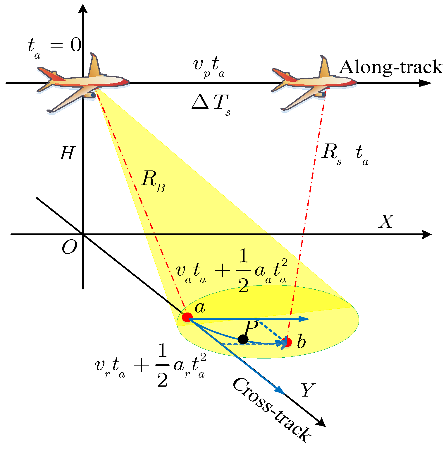
2. Geometric and Signal Model for Ground Manoeuvring Target

The geometric configuration between an airborne platform with velocity $v_p$ at a height of $H$ and a ground manoeuvring target is given in Figure 1. In the slow time $\Delta T_s$, the ground manoeuvring target $P\left(x_{p },y_{p }, z_{p }\right)$ moves from point $a$ to point $b$, where $v_a, a_a$ are the along-track velocity and acceleration, respectively, and $v_r, a_r$ denote the cross-track velocity and acceleration, respectively, as shown in Figure 1, $R_B$ and $R_s\left(t_a\right)$ represent the closest slant range and instantaneous slant range from the radar platform to the ground manoeuvring target, respectively, and $t_a$ denotes the azimuth slow time.

According to Figure 1, for azimuth time $t_a$, the instantaneous coordinates of the radar platform and the ground manoeuvring target can be written as $\left(v_p{t}_a,0,H\right)$ and $\left(v_a{t}_a+a_a{t}_a^2/2, y_p+v_r{t}_a+a_r{t}_a^2/2,0\right)$, respectively. After applying the third-order Taylor series expansion, the instantaneous range $R_s\left(t_a\right)$ is [27]

$$\begin{array}{ll}{R}_s\left(t_a\right)& =\sqrt{{\left(v_p{t}_a-v_a{t}_a-\frac{1}{2}{a}_a{t}_a^2\right)}^2+{\left( y_p+v_r{t}_a+\frac{1}{2}{a}_r{t}_a^2\right)}^2+H^2}\\ & \approx R_B+b_1{t}_a+b_2{t}_a^2+b_3{t}_a^3\end{array}$$

(1)

where $b_1$, $b_2$ and $b_3$ denote the first-, second-, and third-order coefficients of the instantaneous slant, respectively, under the assumption of $\left(v_p-v_a\right)\Delta T_s\ll R_B$ [27], [32,33]. In Equation (1), the detailed expressions of each variable are

$$\begin{array}{c}{R}_B=\sqrt{{\left(y_p\right)}^2+H^2},b_1=\frac{y_p{v}_r}{R_B},b_2=\frac{v_r^2+{\left(v_p-v_a\right)}^2+y_p{a}_r}{2R_B}-\frac{{\left(y_p\right)}^2{v}_r^2}{2R_B^3}\\ b_3=\frac{-a_a\left(v_p-v_a\right)+v_r{a}_r}{2R_B}-\frac{ y_p{v}_r\left[v_r^2+{\left(v_p-v_a\right)}^2+y_p{a}_r\right]}{2R_B^3}+\frac{{\left(y_p\right)}^3{v}_r^3}{2R_B^5}\end{array}$$

(2)

It is interesting to note that the third-order coefficient is considered in the signal model in Equation (2). This term is important to generate clear images because of the increased aperture time in the current SAR systems [27], [32]. The conventional approaches using the second-order signal model are invalid. In what follows, a novel approach for SAR ground manoeuvring target imaging and motion parameter estimation is introduced where the high-order phase signal model is necessary.

Suppose the radar transmits a linear frequency modulated (LFM) signal [7], which is

$${\mathrm{s}}_t\left(t_r\right)=w_r\left(t_r\right)exp\left[j2\pi \left(f_c{t}_r+K_r{t}_r^2/2\right)\right]$$

(3)

where $t_r$ is the range fast-time variable, $f_c$ is the carrier frequency, $K_r$ is the chirp rate of the LFM signal, and, $w_r\left(t_r\right)$ is the range envelope function.

After conducting the Fourier transform (FT) for the variable $t_r$ in Equation (3) and removing the range modulation term, the received echo of the ground manoeuvring target is

$$\begin{array}{c}\text{s}\left(f_r;t_a\right)={\sigma }_s{W}_r\left(f_r\right)w_a\left(t_a\right)exp\left[-j\frac{4\pi \left(f_r+f_c\right)R_s\left(t_a\right)}{c}\right]\\ ={\sigma }_s{W}_r\left(f_r\right)w_a\left(t_a\right)exp\left[-j\frac{4\pi \left(f_r+f_c\right)\left(R_B+b_1{t}_a+b_2{t}_a^2+b_3{t}_a^3\right)}{c}\right] \end{array}$$

(4)

where $f_r$ is the range frequency variable, ${\sigma }_s$ denotes the complex reflective coefficient of the manoeuvring target, $c$ is the speed of light, and $W_r(·)$ and $w_a(·)$ are the range and azimuth envelope functions in the range frequency domain and azimuth time domain, respectively.

Inspecting Equation (4) reveals that the RCM contains three terms: the range walk, range curvature, and high-order $\left(\ge 3\right)$ range migration, and because of their existence, the trajectory of the manoeuvring target spans across different range cells. Therefore, to obtain a well-refocused imaging result of the manoeuvring target, the large RCM and nonstationary DFM must be corrected and compensated in advance.

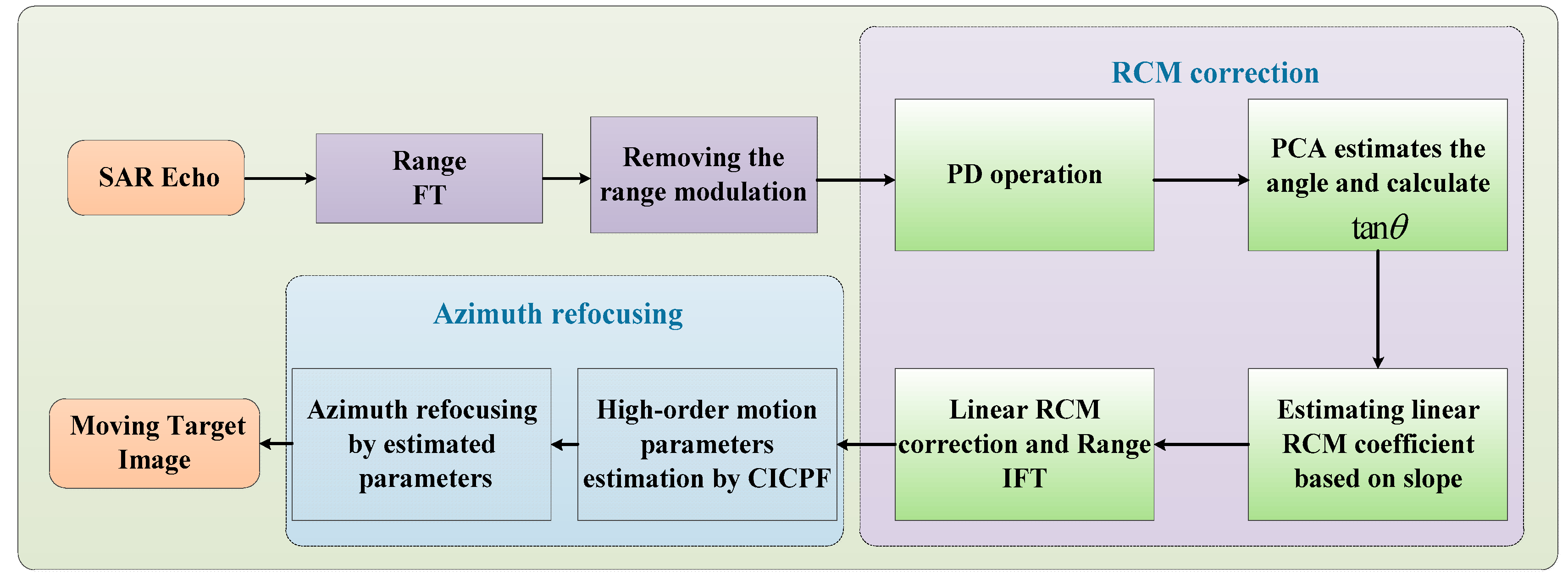
3. Description of the Proposed Method

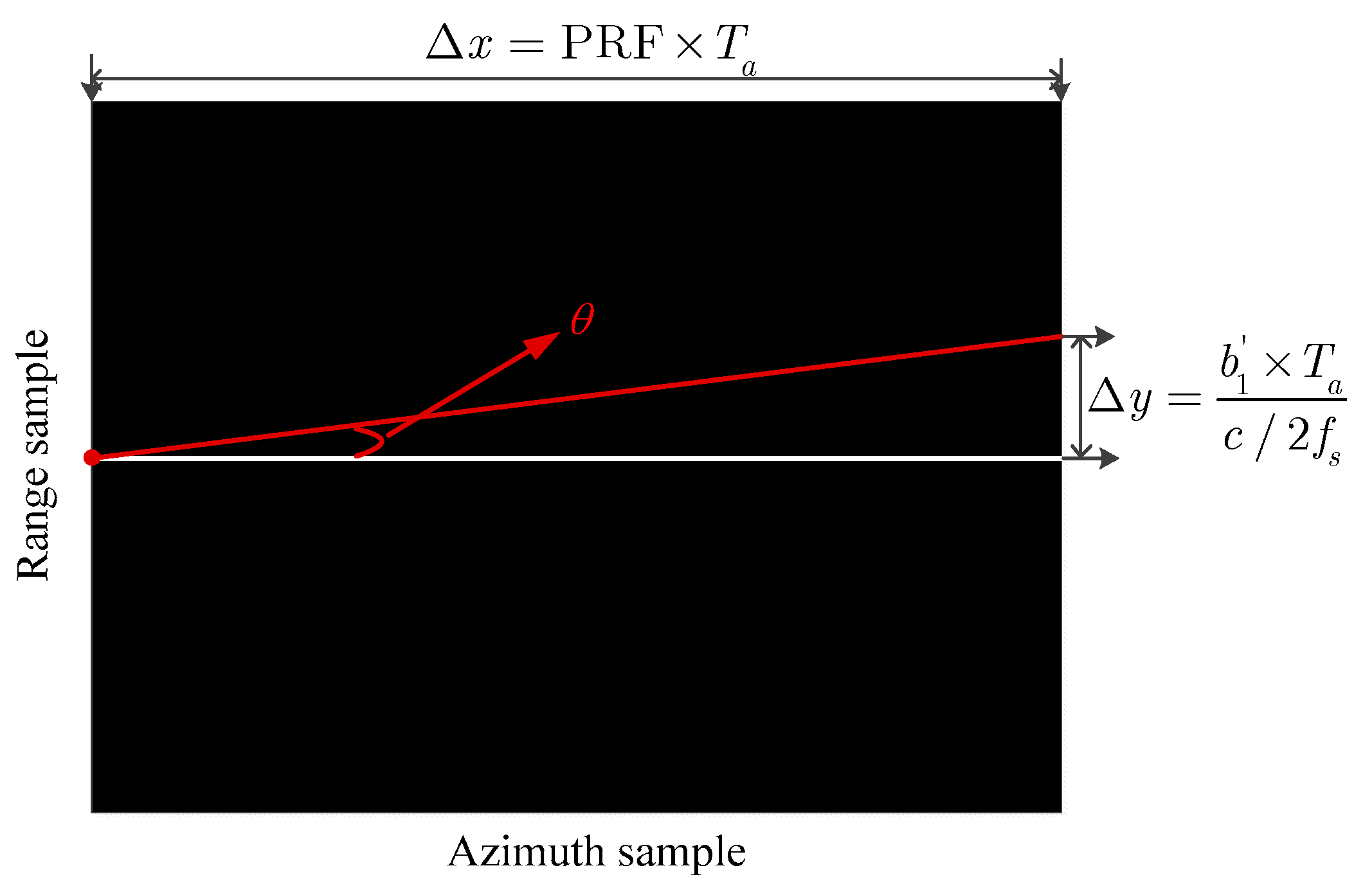
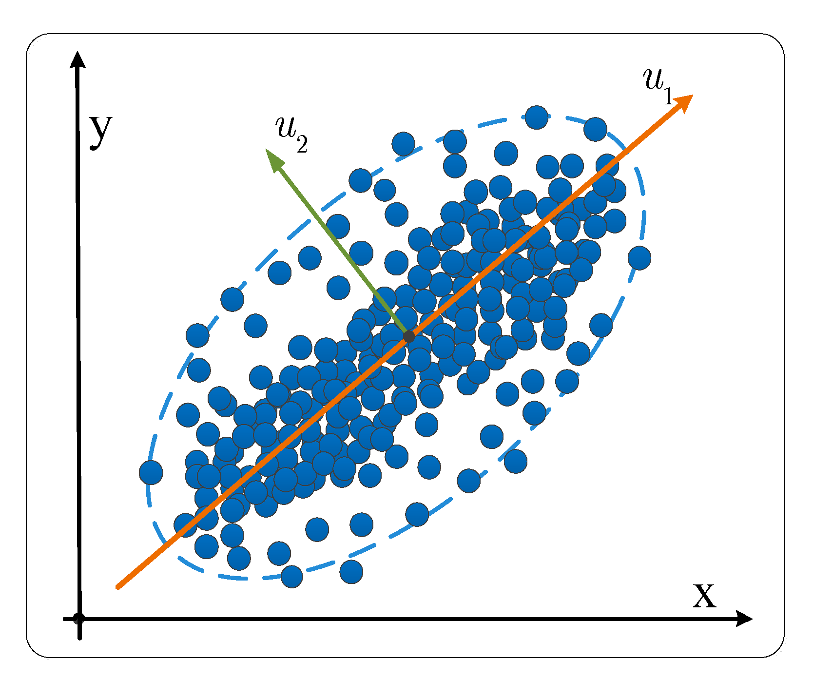
In this section, on the basis of the geometric and signal configuration presented in Section 2, an effective ground manoeuvring target refocusing approach combined with PCA and high-order motion parameter estimation is proposed. Before the time-varying DFM parameter estimation, the RCM correction is introduced.

3.1. RCM Correction

From Equation (4), in each range cell, the signal in terms of the slow-time variable $t_a$ axis can be modelled as a polynomial phase signal (PPS) that is obtained at $f_r=f_r^{\prime }$ as

$$\begin{array}{cc}\hfill s\left(t_a\right)& =s_r\left(f_r=f_r^{\prime };t_a\right)\hfill \\ & ={\sigma }_s{W}_r\left(f_r\right)w_a\left(t_a\right)exp\left[-j\frac{4\pi \left(f_r^{\prime }+f_c\right)\left(R_B+b_1{t}_a+b_2{t}_a^2+b_3{t}_a^3\right)}{c}\right]\hfill \\ & ={\sigma }_s{W}_r\left(f_r\right)w_a\left(t_a\right)exp\left(-j2\pi \left(a_0+a_1{t}_a+a_2{t}_a^2+a_3{t}_a^3\right)\right)\hfill \end{array}$$

(5)

where $a_0=2\left(f_r^{\prime }+f_c\right)R_B/c$, $a_i=2\left(f_r^{\prime }+f_c\right)b_i/c$, and $i=1,2,3$ are the coefficients of the PPS. In Equation (5), the coefficients $a_i,i=0,1,2,3$ are responsible for the RCM and DFM of the ground maneuvering target. This indicates that if we can lower the order in the PPS signal, the RCM and azimuth DFM can be corrected effectively.

From estimation theory, the PD method is widely used to reduce the order in PPS, and the PD is defined by [34,35]

$$\begin{array}{l}{\mathrm{PD}}^1\left[n;{\tau }_1\right]=x\left(n+{\tau }_1\right)x^{*}\left(n-{\tau }_1\right)\\ {\mathrm{PD}}^2\left[n;{\tau }_1,{\tau }_2\right]={\mathrm{PD}}^1\left[n+{\tau }_2;{\tau }_1\right]{\left[{\mathrm{PD}}^1\left[n-{\tau }_2;{\tau }_1\right]\right]}^{*}\\ ⋮\\ {\mathrm{PD}}^Q\left[n;{\tau }_1,{\tau }_2,\cdots ,{\tau }_Q\right]={\mathrm{PD}}^{Q-1}\left[n+{\tau }_Q;{\tau }_1,{\tau }_2,\cdots ,{\tau }_{Q-1}\right]\\ \times {\left[{\mathrm{PD}}^{Q-1}\left[n-{\tau }_Q;{\tau }_1,{\tau }_2,\cdots ,{\tau }_{Q-1}\right]\right]}^{*}\end{array}$$

(6)

where ${\tau }_i,i=1,2\cdots Q$ is the lag variable and $(*)$ is the complex conjugate. The rule of selecting the lag variable ${\tau }_i$ needs to satisfy the constraint of ${\tau }_i=m\mathrm{PRT},m=1,2,3\cdots N$.

After applying Equation (6), the result using the PD technique is

$$\begin{array}{cc}\hfill s_{\mathrm{PD}}\left(f_r;t_a\right)& ={\mathrm{PD}}^1\left[s\left(f_r;t_a\right)\right]=s\left(f_r;t_a+{\tau }_1\right)s{\left(f_r;t_a-{\tau }_1\right)}^{*}\hfill \\ & ={\sigma }_s^{\prime }exp\left[-j\frac{4\pi \left(f_r+f_c\right)}{c}\left(2b_1{\tau }_1+2b_3{\tau }_1^3+4b_2{\tau }_1{t}_a+6b_3{\tau }_1{t}_a^2\right)\right]+\underset{cross-term}{\underbrace{{\mathrm{PD}}_{l,c-terms}\left(f_r;t_a\right)}}\hfill \\ & ={\sigma }_s^{\prime }{\left[W_r\left(f_r\right)\right]}^2{w}_a\left(t_a+{\tau }_1\right)w_a\left(t_a-{\tau }_1\right)\hfill \\ & \times exp\left[\frac{-j4\pi f_r}{c}\left(2b_1{\tau }_1+2b_3{\tau }_1^3+4b_2{\tau }_1{t}_a+6b_3{\tau }_1{t}_a^2\right)\right]\hfill \\ & \times exp\left[\frac{-j4\pi }{\lambda }\left(2b_1{\tau }_1+2b_3{\tau }_1^3+4b_2{\tau }_1{t}_a+6b_3{\tau }_1{t}_a^2\right)\right] +\underset{cross-term}{\underbrace{{\mathrm{PD}}_{l,c-terms}\left(f_r;t_a\right)}}\hfill \end{array}$$

(7)

where ${\sigma }_s^{\prime }={\sigma }_s^2{\left[W_r\left(f_r\right)\right]}^2{w}_a\left(t_a+{\tau }_1\right)w_a\left(t_a-{\tau }_1\right)$ and ${\mathrm{PD}}_{l,c-terms}\left(f_r;t_a\right)$ denotes the cross-term after the PD operation. The terms, $2b_1{\tau }_1+2b_3{\tau }_1^3$, $4b_2{\tau }_1{t}_a$ and $6b_3{\tau }_1{t}_a^2$ are now the RCM and DFM coefficients.

From Equation (7), after PD operation, the RCM is migrated, and the order of the azimuth time-varying DFM is now two. Moreover, the new range curvature $R_{\mathrm{qrcm}}=6b_3{\tau }_1{t}_a^2$ is determined by the coefficient $b_3$. Using the simulation settings in

Table 1. SAR system and target motion parameters.

Parameter	Value
Carrier frequency	10 GHz
Nearest slant range	400 m
Range bandwidth	1 GHz
Pulse repetition frequency	1500 Hz
SAR platform velocity	200 m/s
Along-track velocity	10 m/s
Cross-track velocity	6 m/s
Along-track acceleration	$3\mathrm{m}/s^2$
Cross-track acceleration	$4\mathrm{m}/s^2$

, the maximum value of $R_{\mathrm{qrcm}}$ during the synthesis aperture time is $\max \left\{R_{\mathrm{qrcm}}\left(t_a\right)\right\}={\left|6b_3{\tau }_1{t}_a^2\right|}_{\left|t_a=\pm \frac{T_a}{2},{\tau }_1=8\mathrm{PRT}\right|}=0.002786,$ where the delay variable ${\tau }_1$ is selected as $8\mathrm{PRT}$. Therefore, the range curvature after PD operation can be omitted since it does not exceed half of the range resolution cell of ${\rho }_r=c/B_r=0.15m$, where $B_r$ denotes the transmitted signal bandwidth.

Although the range curvature can be ignored, the linear RCM (that is, the range walk term) determined by $4b_2{\tau }_1{t}_a$ is still out of the range that is allowed and needs to be compensated. There are many approaches that can be utilized to remove the linear RCM term, such as the RT method [14,15,17,18], HT method [16,27], and information entropy [36]. It is well known that these methods can be used to estimate the slope of the linear RCM, which is the basis for its compensation. Another approach uses KT-based methods [7,8,9,10], which are readjusted by interpolation to remove the coupling between the range frequency and the slow time to correct the linear RCM. However, these methods suffer from large computational loads and accuracy loss because of the interpolation used and multidimensional search steps required, which is not suitable for real-time implementation. To overcome the difficulties mentioned above, in this work, an efficient linear RCM correction method based on PCA is proposed by exploiting the geometric information of RCM.

After PD implementation, the energy trajectory of the manoeuvring target is transformed into a straight line in the two-dimensional time domain, and the interaction between the slope and linear RCM is illustrated in Figure 2, where $b_1^{\prime }=4b_2{\tau }_1$ is the linear RCM coefficient in Equation (7), $T_a$ is the moving target time of duration, $f_s$ is the range sample frequency, and $\mathrm{PRF}$ represents the pulse repetition frequency. From Figure 2, the slope of the straight line can be estimated as

$$\tan \widehat{\theta }=\frac{\Delta y}{\Delta x}=\frac{2f_s\times b_1^{\prime }}{\mathrm{PRF}\times c}$$

(8)

where $\widehat{\theta }$ represents the estimation of the angle between the trajectory and the horizontal line. From Equation (8), the linear RCM coefficient $b_1^{\prime }$ can be estimated with the known trajectory slope. That is,

$$b_1^{\prime }=\frac{\mathrm{PRF}\times \tan \widehat{\theta }\times c}{2f_s}.$$

(9)

It is apparent that the estimation for the trajectory slope is the key step. To obtain the slope, the RT method [14,15,17,18], HT method [16,27], and information entropy [36] can be used to obtain the slope. However, all these methods have a heavy computing load, which limits their applications in real-time systems. Therefore, in this work, an efficient linear RCM correction method based on PCA is developed.

PCA is generally used in determining the maximum variance direction of a given data set [37,38], which maps a data set into another one in a new coordinate system, where the first coordinate represents the largest variance of the data set. As depicted in Figure 3, based on this property, the largest variance is represented by the first principal component $u_1$ in the PCA method (the largest variance indicates the maximum dispersion and represents the largest amount of information contained), and the main energy direction of the data set is then determined. It is also interesting to note that targets (military aircraft and ships) in SAR systems always present a unique direction with the largest variance because of their elliptical geometric shapes. Based on this reason, in this work, PCA is utilized to estimate the direction of the main energy of linear RCM, which is one of the main innovations.

Generally, for the target detection problem in SAR systems, the energy of the target is stronger than that of the background after clutter rejection, which means that the SCNR is relatively high. Therefore, the position of the strong scatterer in the target can be obtained by using the energy threshold of the signal. In this work, the threshold $R_{\mathrm{threshold}}$ is set as half of the strongest scatterer energy. Then, by choosing the coordinates of energy points that are greater than $R_{\mathrm{threshold}}$, the database $P$ is formed as

$$P=\left[p_1,p_2,\cdots ,p_L\right]$$

(10)

where $p_i={\left[m_i,n_i\right]}^T$ indicates the range and azimuth coordinate of the $ith$ energy point, and $L$ denotes the number of data points that satisfy the condition.

The mean vector $A\left(M_x,N_y\right)$ for database $P$ is defined as

$$\{\begin{array}{c}{M}_x=\frac{1}{L}{\displaystyle \sum _{i=1}^L}{m}_i\\ N_y=\frac{1}{L}{\displaystyle \sum _{i=1}^L}{n}_i\end{array}$$

(11)

where $M_x$ and $N_y$ denote the mean values of the range and azimuth coordinates, respectively.

The new database $\overline{P}$ is produced by subtracting the mean vector $A$ from the matrix $P$ as

$$\overline{P}=P-A$$

(12)

Constructing a covariance matrix with the database $\overline{P}$ yields

$$C_p=\frac{1}{L}\left(\overline{P}\right){\left(\overline{P}\right)}^T$$

(13)

In particular, $C_p$ is a real symmetric matrix, and the eigenvalue decomposition of $C_p$ can be expressed as

$$C_p=Q\Lambda Q^T$$

(14)

where $\Lambda$ denotes a diagonal matrix with two eigenvalues and $Q$ denotes the corresponding eigenvectors for $\Lambda$. According to the previous analysis and Figure 3, it is known that the eigenvector $\left(m_x,n_y\right)$ corresponding to the largest eigenvalue is the direction of the main axis. Thus, the slope of the trajectory is then calculated as

$$\tan \widehat{\theta }=\frac{n_y}{m_x}$$

(15)

From Equations (9) and (15), the linear RCM coefficient can be accurately estimated, and then, the linear RCM term can be corrected by using the following compensation function $H_{\mathrm{RWM}}$.

$$H_{\mathrm{RWM}}=exp\left(j\frac{4\mathsf{\pi }{b}_1^{\prime }}{c}{f}_r{t}_a\right)$$

(16)

Multiplying Equations (7) and (16) and conducting IFT along the range frequency variable $f_r$, the echo signal can be represented as

$$\begin{array}{cc}\hfill s_2\left(t_a\right)& ={\sigma }_s^{\prime }\sin \mathrm{c}\left\{B_r\left[t_r-\frac{2\left(2b_1{\tau }_1+2b_3{\tau }_1^3\right)}{c}\right]\right\}\hfill \\ & \times exp\left[\frac{-j4\pi }{\lambda }\left(2b_1{\tau }_1+2b_3{\tau }_1^3+4b_2{\tau }_1{t}_a+6b_3{\tau }_1{t}_a^2\right)\right]+\underset{cross-term}{\underbrace{{\mathrm{PD}}_{l,c-terms}\left(t_r;t_a\right)}}.\hfill \end{array}$$

(17)

From Equation (17), after the aforementioned operation, the energy of the ground manoeuvring target is concentrated into the same range gate $R\left(t_a\right)=2b_1{\tau }_1+2b_3{\tau }_1^3$. By doing so, the RCM has been corrected efficiently. In the next section, the CICPF method is introduced to estimate the coefficients of nonstationary DFM.

3.2. Motion Parameter Estimation Using CICPF

From Equation (17), after the RCM correction with efficient PD and PCA operation, the non-stationary DFM signal is expressed as an LFM signal, given by

$$s_3\left(t_m\right)=Aexp\left[j2\pi \left(c_0+c_1{t}_m+c_2{t}_m^2\right)\right]+n\left(t_m\right)$$

(18)

where $A={\sigma }_s^{\prime }$ denotes the signal amplitude, and $c_0=-2\left(2b_1{\tau }_1+2b_3{\tau }_1^3\right)/\lambda$, $c_1=-2\left(4b_2{\tau }_1\right)/\lambda$, $c_2=-2\left(6b_3{\tau }_1\right)/\lambda$, and $n\left(t_m\right)$ denote the interference signal and noise. The key step is to estimate the coefficients of the LFM signal in Equation (18), which is related to the DFM.

For an LFM signal, the cubic phase function (CPF) is defined as [39]

$$\begin{array}{cc}\hfill \mathrm{CPF}\left(t_m;f_{{\tau }_m^2}\right)& ={{\displaystyle \int }}^{}{s}_3\left(t_m+{\tau }_m\right)s_3\left(t_m-{\tau }_m\right)exp\left(-j2\pi f_{{\tau }_m^2}{\tau }_m^2\right)d{\tau }_m^2\hfill \\ & =\underset{auto-terms}{\underbrace{A^{2}exp\left[j4\pi \left(c_0+c_1{t}_m+c_2{t}_m^2\right)\right]{\delta }_{{\tau }_m^2}\left(f_{{\tau }_m^2}-2c_2\right)}} \hfill \\ & \underset{cross-terms}{+\underbrace{{\mathrm{CPF}}_{s,c-terms}\left(t_m;f_{{\tau }_m^2}\right)+{\mathrm{CPF}}_{s,n-terms}\left(t_m;f_{{\tau }_m^2}\right)}}\hfill \end{array}$$

(19)

where ${\tau }_m$ represents the lag-time variable, $f_{{\tau }_m^2}$ denotes the frequency variable in terms of the lag-time variable, and $\delta (\Delta )$ denotes the Dirac delta function. ${\mathrm{CPF}}_{s,c-terms}\left(t_m;f_{{\tau }_m^2}\right)$ and ${\mathrm{CPF}}_{s,n-terms}\left(t_m;f_{{\tau }_m^2}\right)$ represent the cross-terms and the noise term after CPF operation. From Equation (19), it can be seen that the LFM signal is now accumulated in the straight line of $f_{{\tau }_m^2}=2c_2$ in the time–frequency $\left(t_m;f_{{\tau }_m^2}\right)$ domain.

Using the characteristics of the self-term energy distribution along the time axis, the product CPF (PCPF) and integral CPF (ICPF) [40,41] are adopted to perform cross-term and spurious peak suppression. However, these two methods only use partial autoterm energy, and both are noncoherent integrations. In view of the shortcomings of the above two algorithms, we propose to utilize the coherently integrated CPF (CICPF) transform [42] by further exploiting the amplitude and phase information of the signal. With the CICPF, Equation (19) is

$$\begin{array}{cc}\hfill \mathrm{CICPF}\left(f_{t_m};f_{{\tau }_m^2}\right)& ={\mathsf{\Gamma }}_{t_m}\left[\mathrm{CPF}\left(t_m;f_{{\tau }_m^2}\right)\right]\hfill \\ & ={{\displaystyle \int }}^{}\mathrm{CPF}\left(t_m;f_{{\tau }_m^2}\right)exp\left(-j2\pi f_{{\tau }_m^2}{t}_m^2-j2\pi f_{t_m}{t}_m\right)\hfill \\ & =\underset{auto-terms}{\underbrace{\mathrm{g}\left(f_{{\tau }_m^2}=2c_2\right)A^{2}exp\left(4\pi c_0\right){\delta }_{{\tau }_m^2}\left(f_{{\tau }_m^2}-2c_2\right){\delta }_{t_m}\left(f_{t_m}-2c_1\right)}}\hfill \\ & +\underset{cross-terms}{\underbrace{{\mathrm{CICPF}}_{s,c-terms}\left(f_{t_m};f_{{\tau }_m^2}\right)+{\mathrm{CICPF}}_{s,n-terms}\left(f_{t_m};f_{{\tau }_m^2}\right)}}\hfill \end{array}$$

(20)

where ${\mathsf{\Gamma }}_{t_m}$ denotes the CICPF operation, $f_{t_m}$ is the frequency variable about $t_m$, and $\mathrm{g}\left(f_{{\tau }_m^2}=2c_2\right)=exp\left[-j2\pi \left(f_{{\tau }_m^2}-2c_2\right)t_m^2\right]$. It can be seen from Equation (20) that after the CICPF operation, the energy of autoterms accumulates into the peak point of $\left(2c_1,2c_2\right)$ in the $\left(f_{t_m};f_{{\tau }_m^2}\right)$ domain, while the cross-terms and spurious peaks are effectively suppressed. The estimated value of the LFM signal coefficients can be obtained according to the strong point position. Therefore, the nonstationary DFM can be compensated accurately with the estimated parameters ${\widehat{c}}_1$ and ${\widehat{c}}_2$. The corresponding compensation function is designed by

$$H_{\mathrm{Azimuth}}=exp\left[j\frac{4\pi }{\lambda }\left({\widehat{c}}_1{t}_a+{\widehat{c}}_2{t}_a^2\right)\right].$$

(21)

Multiplying Equations (17) and (21) completes the compensation of the azimuth time-varying DFM, and finally, after conducting azimuth FT, the ground manoeuvring target refocusing is

$$\begin{array}{c}{s}_3\left(t_r;t_a\right)={\sigma }_s^{\prime }\sin \mathrm{c}\left\{B_r\left[t_r-\frac{2\left(2b_1{\tau }_1+2b_3{\tau }_1^3\right)}{c}\right]\sin \mathrm{c}\left(B_a{t}_a\right)\right\}\\ \times exp\left[\frac{-j4\pi }{\lambda }\left(2b_1{\tau }_1+2b_3{\tau }_1^3\right)\right] \end{array}$$

(22)

where $B_a$ denotes the azimuth Doppler bandwidth. It is obvious from Equation (22) that the energy of the ground manoeuvring target has been refocused into a sharp peak point. Figure 4 shows the steps of the proposed approach.

4. Experimental Results and Analysis

In this section, using simulated data and airborne real SAR data, the performance of the proposed approach for ground manoeuvring target refocusing is demonstrated, and several approaches are implemented for comparison.

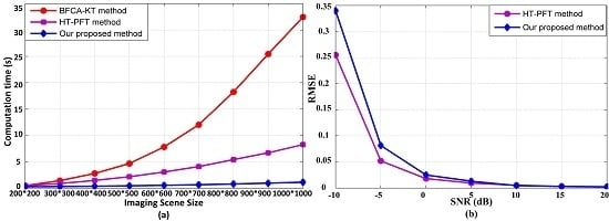
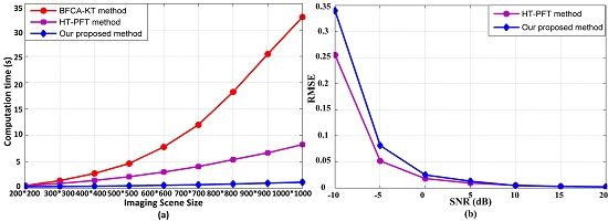
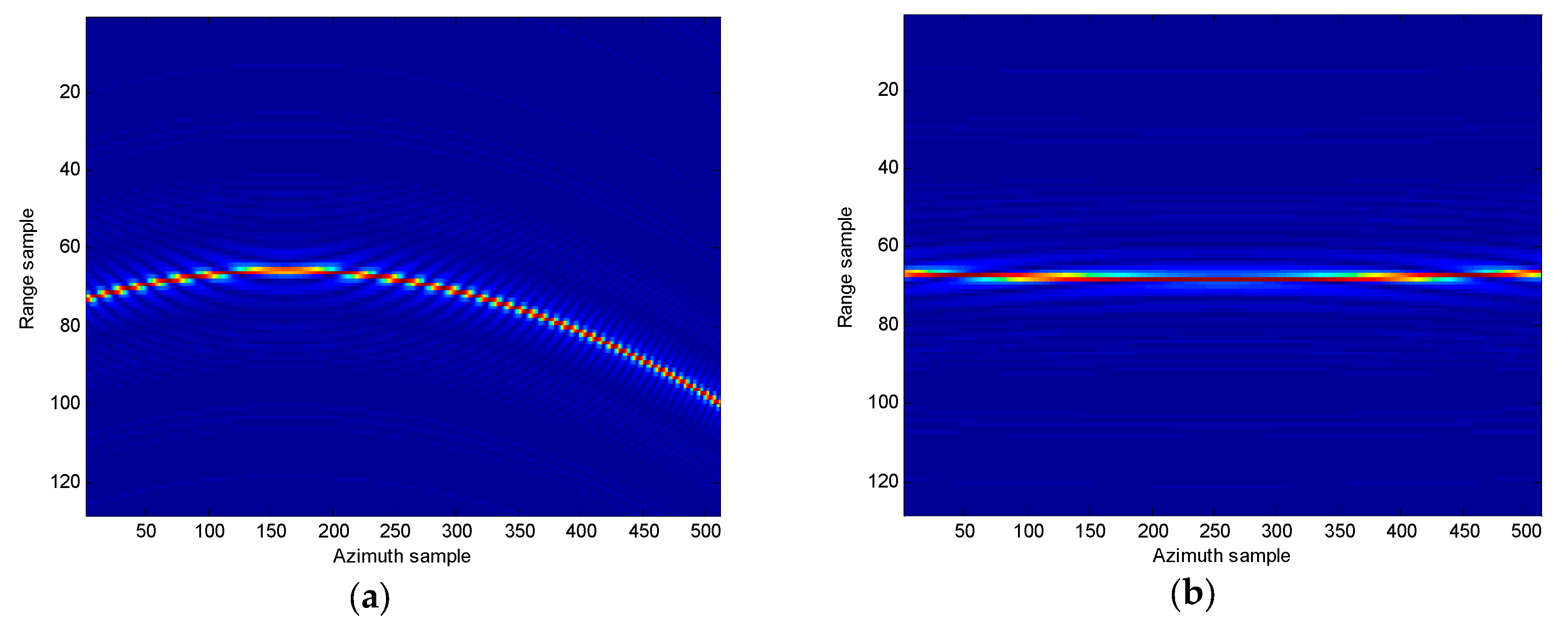
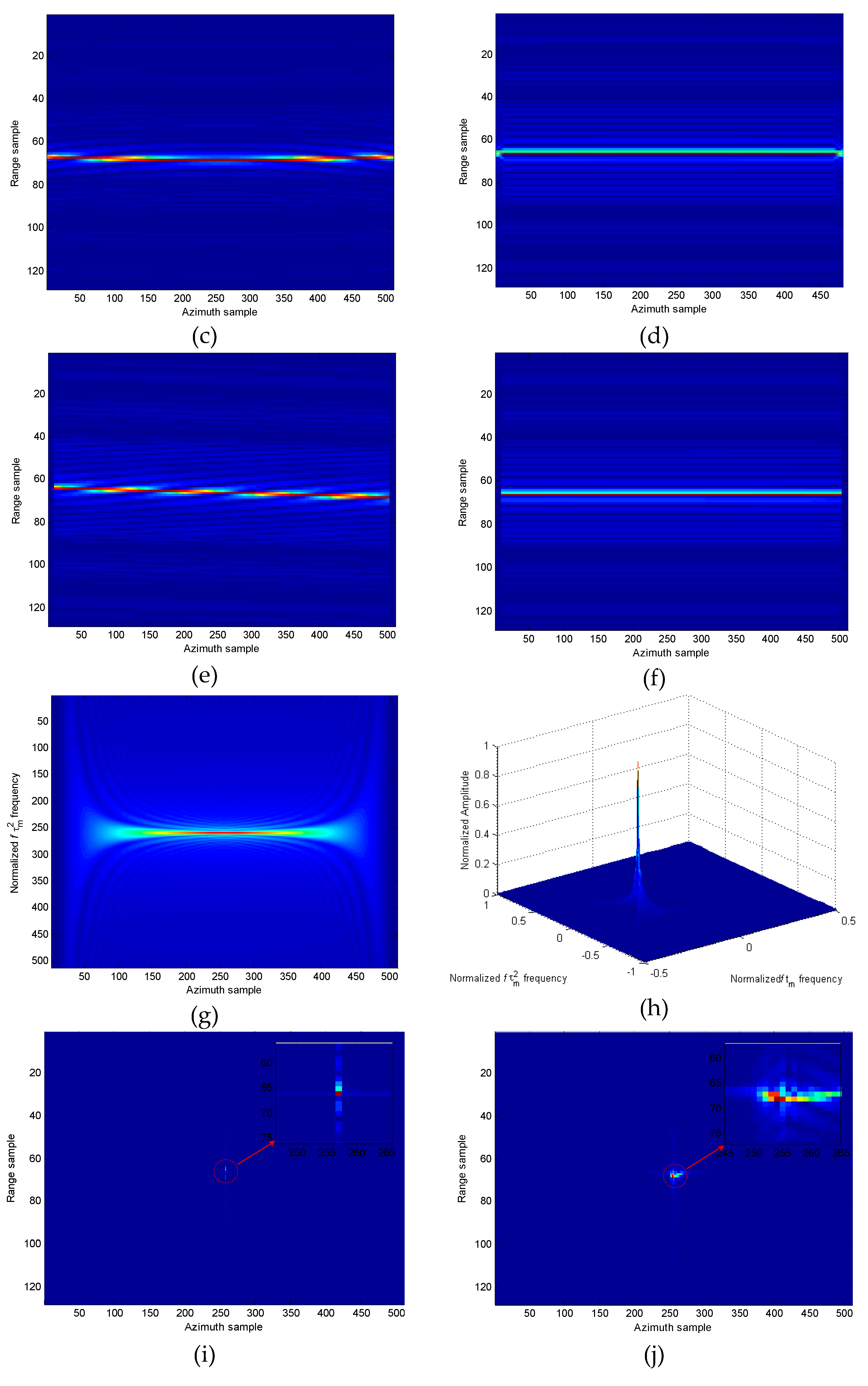
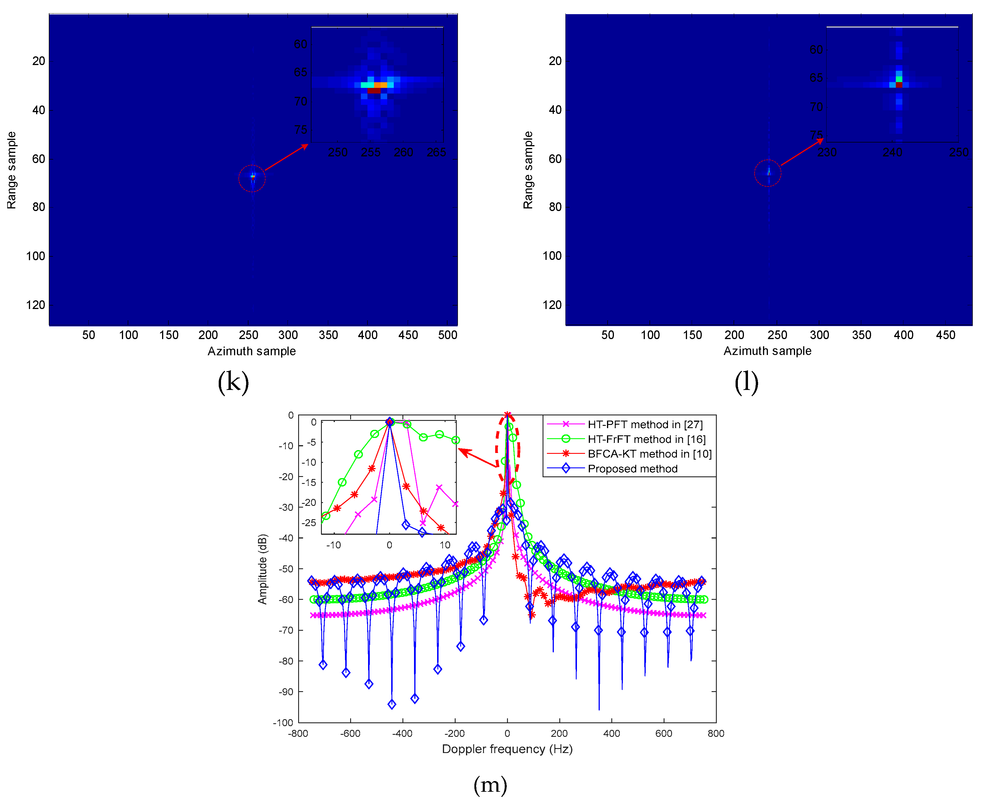
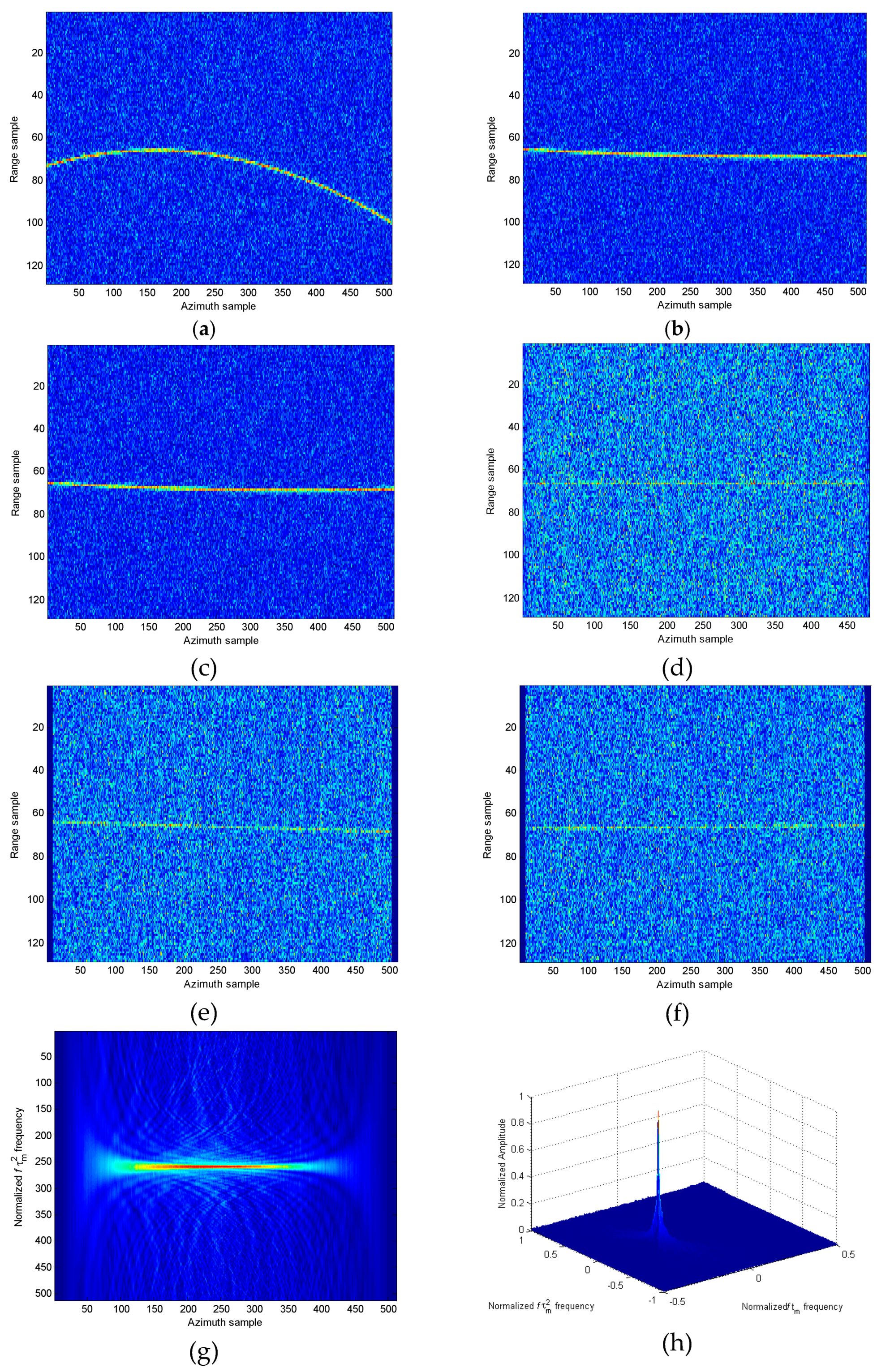
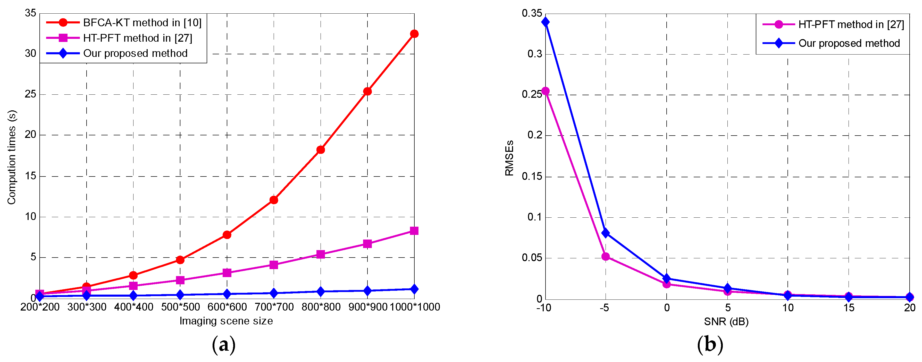
4.1. Simulation Results and Analysis

In this simulation, the simulation settings are given in Table 1. To compare the performances, the results obtained by the HT-FrFT method in [16], HT-PFT method in [27], and BFCA-KT method in [10] are provided as well. Figure 5a indicates the motion trajectories of the manoeuvring target after range compression, from which the motion trajectory shows obvious existing range walk and curvature. The corrected results of the RCM adopting the second-order matching filter and HT in the HT-FrFT method and HT-PFT method are illustrated in Figure 5b,c, respectively. It can be seen that the RCM is not completely corrected due to the existence of the error in radar platform velocity and ground manoeuvring parameters. Figure 5d shows the RCM correction results with the BFCA-KT method in [10]. It can be seen that the RCM has been completely compensated. However, it is well known that these three approaches suffer from large computational loads and accuracy loss, which is unfavourable in real-time implementation. The phase difference (PD) method is utilized to mitigate the effects of RCM and DFM by reducing their order, as shown in Figure 5e, where an RCM trajectory is formed. After PCA operation, the energies of the manoeuvring target are transformed into the same range cell, as demonstrated in Figure 5f, which verifies the effectiveness of the proposed method. After finishing the RCM correction, the processing result of the CPF for the manoeuvring target in the plane $\left(t_m;f_{{\tau }_m^2}\right)$ is depicted in Figure 5g, and it can be seen that, in the time–frequency plane, the energy of the manoeuvring target accumulates along a straight line, which is parallel to the $t_m$ axis. With the CICPF transform, the sole peak is obtained for the energy of the manoeuvring target, as indicated in Figure 5h. The coordinate of the sole peak produces the estimation of the first-order ${\widehat{c}}_1$ and second-order ${\widehat{c}}_2$ motion parameters, the values of which are 1.6693 and –0.0967, respectively. With the estimated parameters, motion compensation is realized, and the well-refocused manoeuvring target is obtained in Figure 5i. Meanwhile, the refocused result with the HT-FrFT method in [16] is depicted in Figure 5j, in which the target is defocused since the third-order DFM coefficient is not considered and the RCM is not fully corrected. Figure 5k illustrates the refocused image generated by the HT-PFT approach in [27], from which the energy of the target still spreads into many range gates since the RCM is not fully corrected. The BFCA-KT approach in [10] provides approximately the same integration quality as the proposed method. However, compared with the BFCA-KT approach, the proposed method has a great advantage in computational cost reduction. Figure 5m illustrates the comparison results of the azimuth profiles obtained with the four methods, it can be seen that the proposed method has a better refocusing performance than the others.

To demonstrate the anti-noise performance of the proposed algorithm, a moving manoeuvring target with a low SNR of –8 dB is generated. In Figure 6a, the result after range compression is provided. The range walk corrections obtained by the HT-FrFT method in [16] and the HT-PFT method in [27] are demonstrated in Figure 6b,c. It can be seen that the RCM is not fully corrected in this case. Figure 6d shows the RCM correction results with the BFCA-KT method in [10], and it can be seen that the RCM has been compensated. After applying the PD operation, the range curvature has been removed, as demonstrated in Figure 6e. Figure 6f shows the RCM correction results with the PCA method. After correcting the RCM, the motion trajectory has been slightly tilted since the PCA is unstable under the low SNR. The CPF and CICPF results are depicted in Figure 6g,h, respectively. Following motion compensation, the well-refocused result for the manoeuvring target is obtained in Figure 6i. The focusing results obtained by the HT-FrFT method in [16], HT-PFT method in [27], BFCA-KT method in [10] and the proposed method are depicted in Figure 6j–l. It is worth noting that the proposed method has better refocusing results than the HT-FrFT method in [16] and the HT-PFT method in [27], and the BFCA-KT approach has the same integration quality as the proposed method. However, compared with the BFCA-KT approach, as discussed earlier, the proposed method has a great advantage in computational cost. Figure 6m presents the comparison results of the azimuth profiles, it can be seen that the proposed method has better refocusing results, which also validate the effectiveness of the proposed method.

To compare the computational complexities of the HT-PFT method, BFCA-KT method, and our proposed method, the running times with different scene sizes are provided in Figure 7a, where MATLAB is used on an Intel Double-core processor with a CPU clocked frequency of 3.0 GHz, 8 GB of memory, and a Windows 10 operating system. Figure 7a confirms that the computational time of the proposed method is much less than that of the HT-PFT and BFCA-KT methods because of avoiding the multidimensional search operation in HT and interpolation operation in KT. Since the slope of trajectory can be estimated by the HT and PCA method, which is related to the coefficient of the linear RCM, the root mean square errors (RMSEs) of trajectory slope estimation in the HT method and proposed PCA method against SNR are given in Figure 7b, where the RMSE values are calculated by averaging 100 independent experiments. Figure 7b shows that the RMSEs of the HT-PFT method are slightly lower than those of our proposed method in the low SNR region, and the RMSEs of both methods decrease as the SNR increases. However, the proposed method has low computational complexity. Therefore, judging from the performance and computational cost, the proposed method achieves a good trade-off.

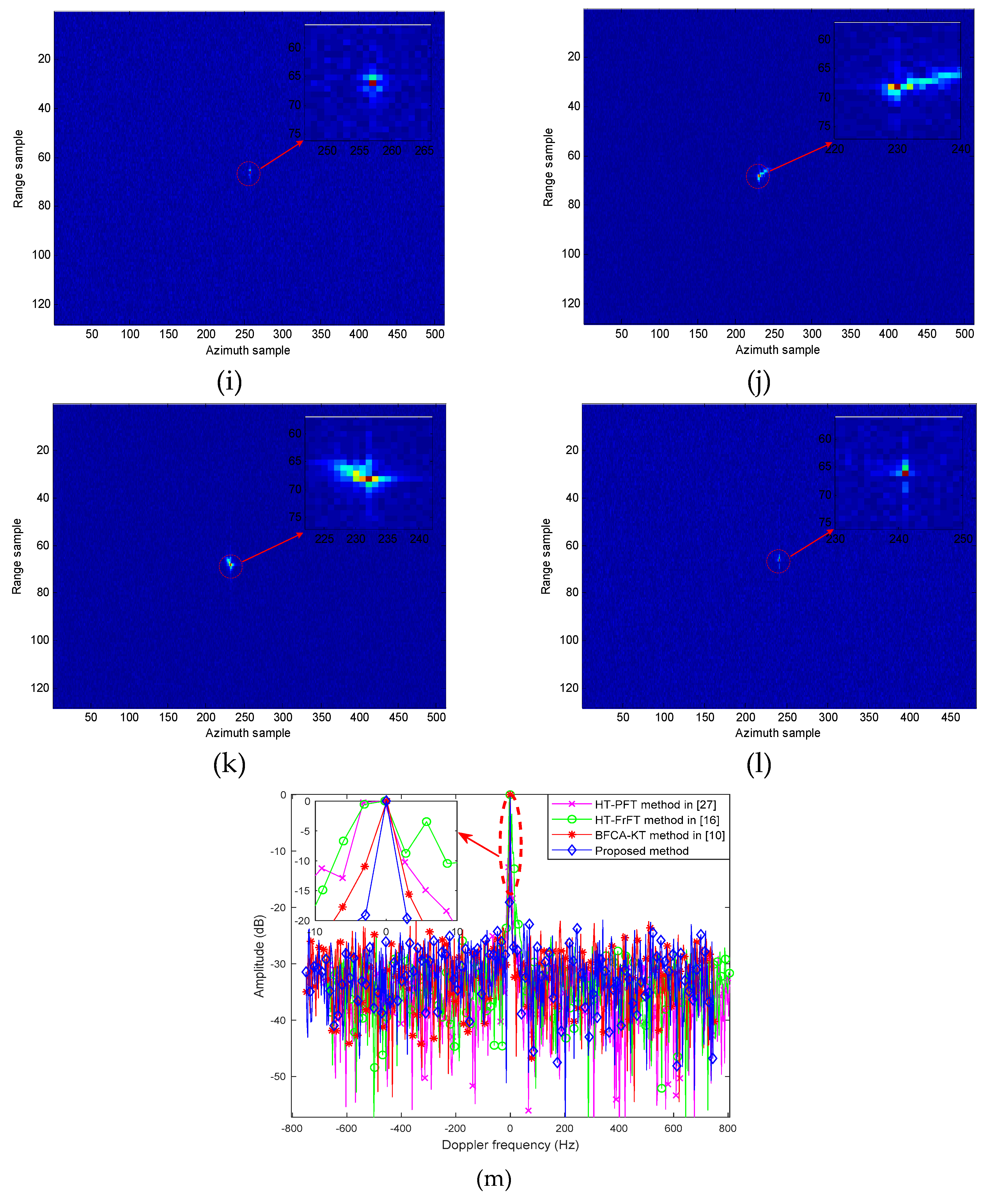
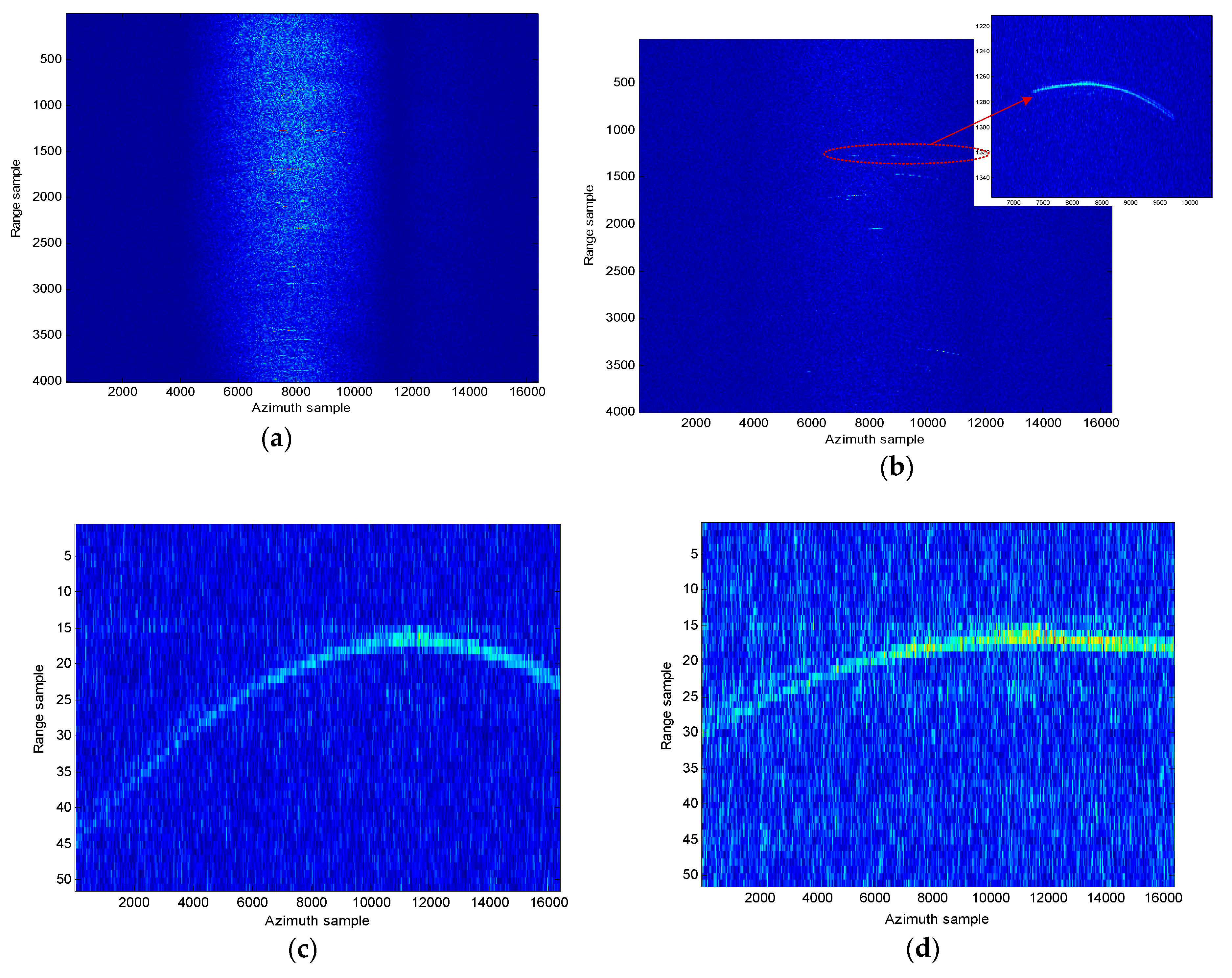
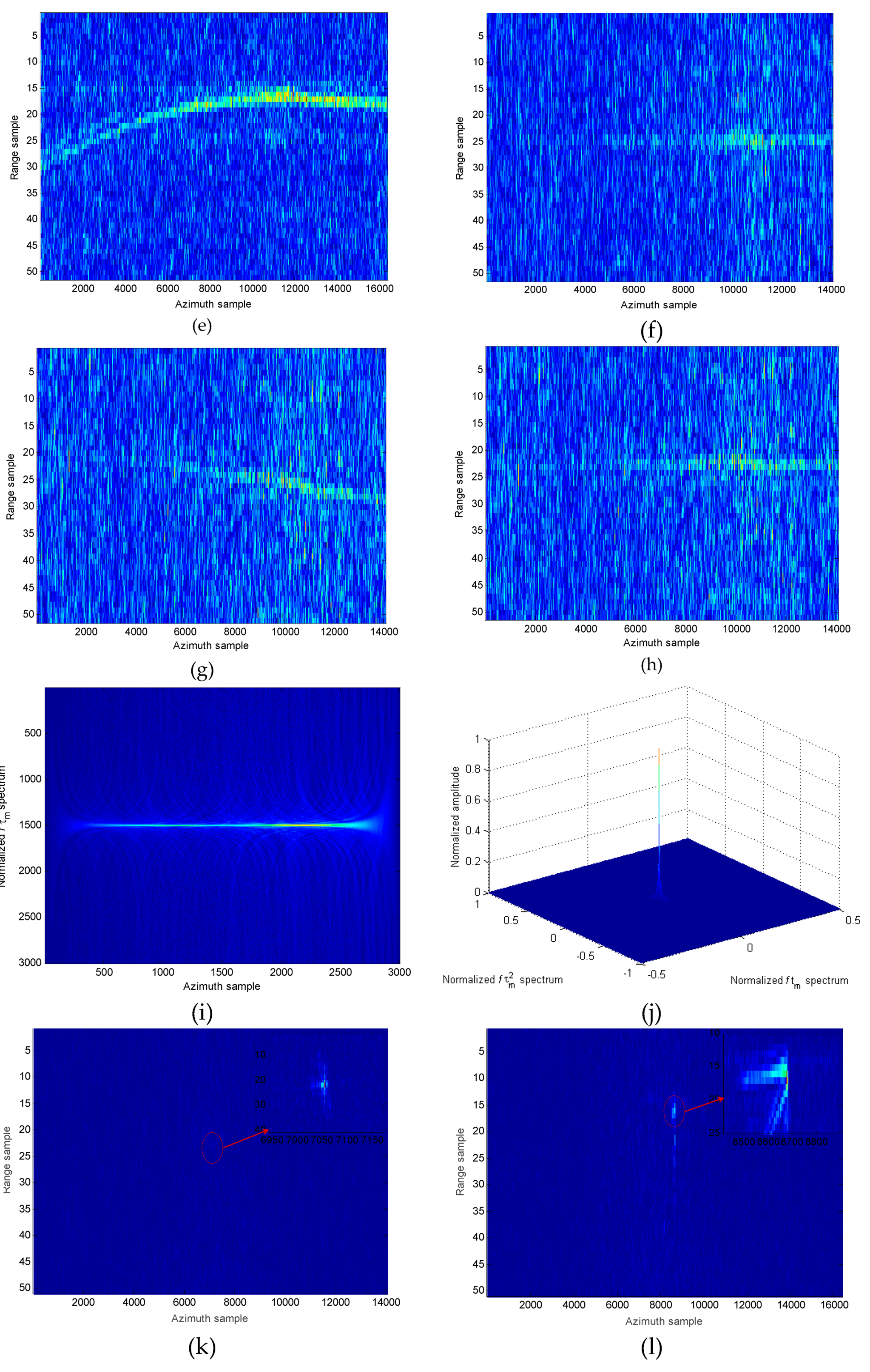
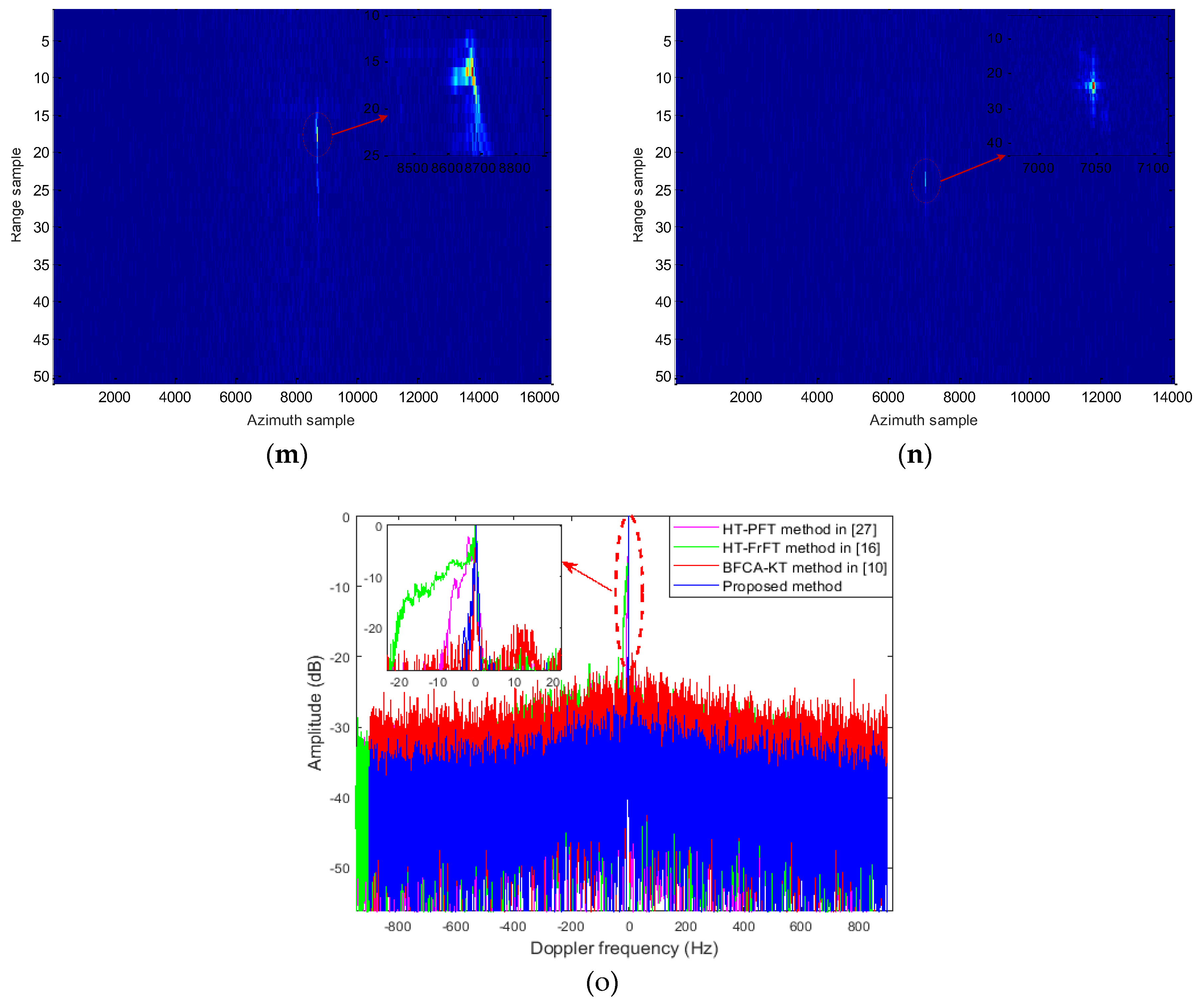
4.2. Measured Data Results and Analysis

In this section, the measured data are utilized to demonstrate the performance of the proposed approach. The SAR data were gathered by a C-band radar in the broadside mode in which the platform moves with a velocity of 130 m/s at an altitude of 8.1 km; the remaining SAR system settings are provided in

Table 2. C-band real radar system parameters.

Parameter	Value
Carrier frequency	5.4 GHz
Range bandwidth	210 MHz
Range sampling frequency	267 MHz
Pulse repetition frequency	1800 Hz
Pulse duration time	10 µs
SAR platform velocity	130 m/s

. The Doppler ambiguities do not occur since the cross-track velocities of moving targets are less than 25 m/s, which is the maximum baseband velocity. Figure 8a,b demonstrates the clutter and target spectra before and after clutter suppression, respectively, where clutter suppression is realized by using the EFA method [43,44,45]. From these figures, after clutter reduction, the moving targets are visible, but they are blurred because of the RCM and DFM. To further show the performances of competing methods, the target inside of the ellipse is considered. Before range migration compensation, Figure 8c depicts the motion trajectories of the manoeuvring target, and a rounded line occurs in the range and azimuth time domains. For the HT-FrFT and HT-PFT methods, the range curvature is compensated using a second-order matching function, and the rotation angle in terms of range walk is then estimated and compensated using the HT. However, the RCM is not fully corrected, as shown in Figure 8d,e. Figure 8f illustrates the RCM correction results obtained by the BFCA-KT method, where the energy of the target is transformed into the same range cell. After applying the PD method, the range curvature has been removed, and a straight slope trajectory is obtained, suggesting the effectiveness of the PD, as depicted in Figure 8g. The range walk correction result via the efficient PCA method is provided in Figure 8h, which verifies the proposed method. The CPF result of the ground moving target is shown in Figure 8i. One observes that the target’s energy does accumulate into a straight line, which is parallel to the $t_m$ axis. By utilizing the CICPF, the target’s energy is now focused as the sole peak, depicted in Figure 8j, where the position of the peak gives the estimations of the first- and second-order motion coefficients, and the values are 0.7292 and 0.0223. After compensating DFM using the estimated parameters, the refocused result for the ground manoeuvring target is obtained by the proposed method in Figure 8k, where a well-refocused result is obtained, thus validating the proposed method. The result generated by HT-FrFT is given in Figure 8l, where the target is blurred due to ignoring the third-order DFM coefficient and the residual RCM. The result generated by the HT-PFT approach is shown in Figure 8m, from which the target is not well refocused because the range curvature has not been completely corrected. The result obtained by the BFCA-KT approach is shown in Figure 8n, and it should be noted that the energy of the ground manoeuvring target is well refocused into a sharp peak. The azimuth profiles obtained by the four methods is presented in Figure 8o, it is obvious that our proposed method can require a better performance, which is consistent with the theoretical analysis above.

5. Discussion

In this section, a computational complexity comparison of the proposed method with the BFCA-KT method in [10], HT-FrFT method in [16], and HT-PFT method in [27] is now provided. In this analysis, the range dimension sampling number is $N_r$, and $N_a$ denotes the azimuth sampling number.

The computational load of the BFCA-KT approach in [10] contains the following steps. First, the deramp operation is adopted to remove the range curvature effect with a computational cost of $O\left(N_r{N}_a\right)$, and then, the KT operation is applied to conduct a range walk compensation with a computational cost of $\mathrm{O}\left(2\left(2N_{\mathrm{Ker}}-1\right)N_r{N}_a\right)$, where $N_{Ker}$ is the length of the interpolation kernel. Finally, the CICPF is initiated with a computational cost of $O\left[N_r\left(2N_{a}lo{g}_2{N}_a\right)\right]$. Finally, the total computational cost of the BFCA-KT method is

$$C_{\mathrm{BFCA}-\mathrm{KT}}=O\left(N_r{N}_a+2\left(2N_{\mathrm{Ker}}-1\right)N_r{N}_a+2N_r{N}_{a}lo{g}_2{N}_a\right).$$

(23)

The implementation steps of the HT-FrFT method [16] generally contain RCM correction utilizing the matching filter and HT, and the FrFT is utilized to estimate and compensate the DFM. The computational complexity of range curve correction by the second-order matching function is $O\left(N_r{N}_a\right)$, and the computational complexity of range walk compensation with HT is $O\left(N_r{N}_a^2\right)$. In FrFT-based DFM coefficient estimation, the computational complexity of the FrFT is $O\left(N_{\mathrm{FrFT}}{N}_{a}lo{g}_2{N}_a\right)$, where ${\mathrm{N}}_{\mathrm{FrFT}}$ denotes the scanning number of the FrFT. As a result, the total computational complexity of the HT-FrFT method is

$$C_{\mathrm{HT}-\mathrm{FrFT}}=O\left(2N_r{N}_a+N_r{N}_a^2+N_{FrFT}{N}_{a}lo{g}_2{N}_a\right).$$

(24)

For the HT-PFT algorithm in [27], the steps include range curve correction and HT and PFT operations. First, the computational complexity of the range curve corrected by a matching function is $O\left(N_r{N}_a\right)$. Second, an HT is employed to obtain the estimation of the trajectory slope for the range walk compensation with a computational cost of $O\left(N_r{N}_a^2\right)$. Finally, the azimuth DFM is compensated by PFT with a computational cost of $N_r{N}_{a2}{N}_{a3}O\left(2N_{a}lo{g}_2{N}_a\right)$, where $N_{a2}$ and $N_{a3}$ are the searching times of second-order and third-order coefficient estimation. As a consequence, the total computational complexity of the HT-PFT approach is

$$C_{\mathrm{HT}-\mathrm{PFT}}=O\left(2N_r{N}_a+N_r{N}_a^2+2N_r{N}_{a2}{N}_{a3}{N}_{a}lo{g}_2{N}_a\right).$$

(25)

According to the imaging flowchart in Figure 4, the proposed method requires the following steps. First, the computational complexity of the range curve corrected by the PD operation is $O\left(N_r{N}_a\right)$. Then, a PCA method involving covariance matrix construction and eigen decomposition is utilized to compensate for the range walk. In this work, $\mathrm{D}$ represents the dimension, and $\mathrm{D}=2$,$\mathrm{L}$ is the total number of scattering centres. The computational cost of the covariance matrix construction requires $O\left(L{D}^2\right)$. Using singular value decomposition (SVD), eigen decomposition is conducted with a computational cost of at most $O\left(D^3\right)$. The computational complexity of range walk correction is thus $O\left(L{D}^2+D^3\right)$. Finally, the CICPF is performed to estimate DFM coefficients with a computational cost of $N_{r}O\left(2N_{a}lo{g}_2{N}_a\right)$. Finally, the total computational cost of the proposed approach is

$$C_{\mathrm{proposed}}=O\left(2N_r{N}_a+L{D}^2+D^3+2N_r{N}_{a}lo{g}_2{N}_a\right).$$

(26)

According to Equations (23)–(26), it is seen that the proposed approach has an obvious advantage in terms of the computational cost compared with the BFCA-KT, HT-FrFT, and HT-PFT methods because of avoiding interpolation and multidimensional search operations.

6. Conclusions

In this paper, a fast SAR refocusing algorithm for ground manoeuvring targets based on PD and PCA combined with the CICPF method is presented. In the proposed approach, first, the efficient PD operation and PCA are utilized to correct the RCM, and then, the energy of the manoeuvring target is concentrated into one range gate. Second, with the motion parameters obtained by the CICPF approach, the well-reconstructed image of the manoeuvring target is thus realized. From comparisons, the proposed method presents an obvious advantage in computational cost because it avoids the multidimensional search and interpolation process. The anti-noise performance is also enhanced by fully exploiting the 2-D coherent accumulation characteristics for estimating motion parameters. Finally, the effectiveness of the method is verified by theoretical analysis, simulations, and measured data processing results.

References

1. Wong, F.H.; Yeo, T.S. New application of nonlinear chirp scaling in SAR data processing. IEEE Trans. Geosci. Remote Sens. 2001, 39, 946–953. [Google Scholar] [CrossRef]
2. Kim, A.J.; Dogan, S.; Fisher, J.W.; Moses, R.L.; Willsky, A.S. Attributing scatterer anisotropy for model-based ATR. In Algorithms for Synthetic Aperture Radar Imagery VII; International Society for Optics and Photonics: Bellingham, WA, USA, 2000; Volume 4053, pp. 176–189. [Google Scholar]
3. Sadjadi, F.A. New experiments in inverse synthetic aperture radar image exploitation for maritime surveillance. In Automatic Target Recognition XXIV; SPIE Defense + Security: Baltimore, MD, USA, 2014. [Google Scholar]
4. Noviello, C.; Fornaro, G.; Martorella, M. Focused SAR image formation of moving targets based on Doppler parameter estimation. IEEE Trans. Geosci. Remote Sens. 2015, 53, 3460–3470. [Google Scholar] [CrossRef]
5. Li, Z.; Wu, J.; Huang, Y.; Sun, Z.; Yang, J. Ground-moving target imaging and velocity estimation based on mismatched compression for bistatic forward-looking SAR. IEEE Trans. Geosci. Remote Sens. 2016, 54, 3277–3291. [Google Scholar] [CrossRef]
6. Tian, J.; Cui, W.; Xia, X.; Wu, S. Parameter estimation of ground moving targets based on SKT-DLVT processing. IEEE Trans. Comput. Imaging 2016, 2, 13–26. [Google Scholar] [CrossRef] [Green Version]
7. Perry, R.P.; DiPietro, R.C.; Fante, R.L. SAR imaging of moving targets. IEEE Trans. Aerosp. Electron. Syst. 1999, 35, 188–200. [Google Scholar] [CrossRef]
8. Huang, P.; Liao, G.; Yang, Z.; Xia, X.; Ma, J.; Zhang, X. A fast SAR imaging method for ground moving target using a second-order WVD transform. IEEE Trans. Geosci. Remote Sens. 2016, 54, 1940–1956. [Google Scholar] [CrossRef]
9. Zhu, D.; Li, Y.; Zhu, Z. A keystone transform without interpolation for SAR ground moving-target imaging. IEEE Trans. Geosci. Remote Sens. Lett. 2007, 4, 18–22. [Google Scholar] [CrossRef]
10. Huang, P.; Xia, X.; Liao, G.; Yang, Z. Ground Moving Target Imaging Based on Keystone Transform and Coherently Integrated CPF With a Single-Channel SAR. IEEE J. Sel. Top. Appl. Earth Obs. Remote Sens. 2017, 10, 5686–5694. [Google Scholar] [CrossRef]
11. Zhou, F.; Wu, R.; Xing, M.; Bao, Z. Approach for single channel SAR ground moving target imaging and motion parameter estimation. IET Radar Sonar Navig. 2007, 1, 59–66. [Google Scholar] [CrossRef]
12. Kirkland, D. Imaging moving targets using the second-order keystone transform. IET Radar Sonar Navig. 2011, 5, 902–910. [Google Scholar] [CrossRef]
13. Li, G.; Xia, X.; Peng, Y. Doppler keystone transform: An approach suitable for parallel implementation of SAR moving target imaging. IEEE Geosci. Remote Sens. Lett. 2008, 5, 573–577. [Google Scholar] [CrossRef]
14. Xu, J.; Yu, J.; Peng, Y.; Xia, X. Radon–Fourier transform for radar target detection, I: Generalized Doppler filter bank. IEEE Trans. Aerosp. Electron. Syst. 2011, 47, 1186–1202. [Google Scholar] [CrossRef]
15. Chen, X.; Guan, J.; Liu, N.; He, Y. Maneuvering target detection via Radon-fractional Fourier transform-based long-time coherent integration. IEEE Trans. Signal Process. 2014, 62, 939–953. [Google Scholar] [CrossRef]
16. Yang, J.; Liu, C.; Wang, Y. Detection and imaging of ground moving targets with real SAR data. IEEE Trans. Geosci. Remote Sens. 2015, 53, 920–932. [Google Scholar] [CrossRef]
17. Li, W.; Wang, X.; Wang, G. Scaled Radon-Wigner transform imaging and scaling of maneuvering target. IEEE Trans. Aerosp. Electron. Syst. 2010, 46, 2043–2051. [Google Scholar] [CrossRef]
18. Raihan, S.M.; Abeysekera, S.S. Efficient wideband signal parameter estimation using a radon-ambiguity transform slice. IEEE Trans. Aerosp. Electron. Syst. 2007, 43, 673–688. [Google Scholar]
19. Zhu, S.; Liao, G.; Qu, Y.; Zhou, Z.; Liu, X. Ground moving targets imaging algorithm for synthetic aperture radar. IEEE Trans. Geosci. Remote Sens. 2011, 49, 462–477. [Google Scholar] [CrossRef]
20. Zhang, X.; Liao, G.; Zhu, S.; Zeng, C.; Shu, Y. Geometry-information-aided efficient radial velocity estimation for moving target imaging and location based on Radon transform. IEEE Trans. Geosci. Remote Sens. 2015, 53, 1105–1117. [Google Scholar] [CrossRef]
21. Lv, G.; Li, Y.; Wang, G.; Zhang, Y. Ground moving target indication in SAR images with symmetric Doppler views. IEEE Trans. Geosci. Remote Sens. 2016, 54, 533–543. [Google Scholar] [CrossRef]
22. Chen, V.; Ling, H. Joint time-frequency analysis for radar signal and image processing. IEEE Signal Process. Mag. 1999, 16, 81–93. [Google Scholar] [CrossRef]
23. Kersten, P.R.; Jansen, R.W.; Luc, K.; Ainsworth, T.L. Motion analysis in SAR images of unfocused objects using time-frequency methods. IEEE Geosci. Remote Sens. Lett. 2007, 4, 527–531. [Google Scholar] [CrossRef]
24. Jeong-Won, P.; Joong-Sun, W. An efficient method of Doppler parameter estimation in the time-frequency domain for a moving object from TerraSAR-X data. IEEE Trans. Geosci. Remote Sens. 2011, 49, 4771–4787. [Google Scholar] [CrossRef]
25. Porat, B.; Benjamin, F. Asymptotic statistical analysis of the high-order ambiguity function for parameter estimation of polynomial-phase signals. IEEE Trans. Inf. Theory 1996, 42, 995–1001. [Google Scholar] [CrossRef]
26. Barbarossa, S.; Di Lorenzo, P.; Vecchiarelli, P. Parameter estimation of 2D multi-component polynomial phase signals: An application to SAR imaging of moving targets. IEEE Trans. Signal Process. 2014, 62, 4375–4389. [Google Scholar] [CrossRef]
27. Yang, J.; Liu, C.; Wang, Y. Imaging and parameter estimation of fast-moving targets with single-antenna SAR. IEEE Trans. Geosci. Remote Sens. 2014, 11, 529–533. [Google Scholar] [CrossRef]
28. Sharma, J.; Gierull, C.H.; Collins, M.J. Compensating the effects of target acceleration in dual-channel SAR-GMTI. IEE Proc. Radar Sonar Navig. 2006, 153, 53–62. [Google Scholar] [CrossRef]
29. Huang, P.; Liao, G.; Yang, Z.; Xia, X.; Ma, J. Ground maneuvering target imaging and high-order motion parameter estimation based on second-order Keystone and generalized Hough-HAF transform. IEEE Trans. Geosci. Remote Sens. 2017, 55, 320–335. [Google Scholar] [CrossRef]
30. Xu, J.; Xia, X.; Peng, S.; Yu, J.; Peng, Y.; Qian, L. Radar maneuvering target motion estimation based on generalized Radon–Fourier transform. IEEE Trans. Signal Process. 2012, 60, 6190–6201. [Google Scholar]
31. Kong, L.; Li, X.; Cui, G.; Yi, W.; Yang, Y. Coherent integration algorithm for a maneuvering target with high-order range migration. IEEE Trans. Signal Process. 2015, 63, 4474–4486. [Google Scholar] [CrossRef]
32. Yang, J.; Zhang, Y. An airborne SAR moving target imaging and motion parameters estimation algorithm with azimuth-dechirping and the second-order Keystone transform applied. IEEE J. Sel. Top. Appl. Earth Obs. Remote Sens. 2015, 8, 3967–3976. [Google Scholar] [CrossRef]
33. Yang, J.; Zhang, Y.; Kang, X. A Doppler ambiguity tolerated algorithm for airborne SAR ground moving target imaging and motion parameters estimation. IEEE Geosci. Remote Sens. Lett. 2015, 12, 2398–2402. [Google Scholar] [CrossRef]
34. Li, D.; Zhan, M.; Liu, H.; Liao, Y.; Liao, G. A Robust Translational Motion Compensation Method for ISAR Imaging Based on Keystone Transform and Fractional Fourier Transform Under Low SNR Environment. IEEE Trans. Aerosp. Electron. Syst. 2017, 53, 2140–2156. [Google Scholar] [CrossRef]
35. Barbarossa, S.; Scaglione, A.; Giannakis, G.B. Product high-order ambiguity function for multicomponent polynomial-phase signal modeling. IEEE Trans. Signal Process. 1998, 46, 691–708. [Google Scholar] [CrossRef]
36. Li, X.; Liu, G.; Ni, J. Autofocusing of ISAR images based on entropy-minimization. IEEE Trans. Aerosp. Electron. Syst. 1999, 35, 1240–1252. [Google Scholar] [CrossRef]
37. Kang, J.; Kang, B.; Kim, K. ISAR cross-range scaling using iterative processing via principal component analysis and bisection algorithm. IEEE Trans. Signal Process. 2016, 64, 3909–3918. [Google Scholar] [CrossRef]
38. Partridge, M.; Calvo, R.A. Fast dimensionality reduction and simple PCA. Intell. Data Anal. 1998, 2, 203–214. [Google Scholar] [CrossRef]
39. O’Shea, P. A fast algorithm for estimating the parameters of a quadratic FM signal. IEEE Trans. Signal Process. 2004, 52, 385–393. [Google Scholar] [CrossRef] [Green Version]
40. Wang, P.; Yang, J. Multicomponent chirp signals analysis using product cubic phase function. Dig. Signal Process. 2006, 16, 654–669. [Google Scholar] [CrossRef]
41. Wang, P.; Li, H.; Djurovic, I.; Himed, B. Integrated cubic phase function for linear FM signal analysis. IEEE Trans. Aerosp. Electron. Syst. 2010, 46, 963–977. [Google Scholar] [CrossRef]
42. Li, D.; Zhan, M.; Su, J.; Liu, H.; Zhang, X.; Liao, G. Performances analysis of coherently integrated CPF for LFM signal under low SNR and its application to ground moving target imaging. IEEE Geosci. Remote Sens. 2017, 55, 6402–6419. [Google Scholar] [CrossRef]
43. Xu, G.; Gao, Y.; Li, J.; Xing, M. A Review on InSAR Phase Denoising. IEEE Geosci. Remote Sens. Mag. 2019. [Google Scholar] [CrossRef] [Green Version]
44. Li, D.; Gui, X.; Liu, H.; Su, J.; Xiong, H. An ISAR Imaging Algorithm for Maneuvering Targets With Low SNR Based on Parameter Estimation of Multicomponent Quadratic FM Signals and Nonuniform FFT. IEEE J. Sel. Top. Appl. Earth Obs. Remote Sens. 2016, 12, 5688–5702. [Google Scholar] [CrossRef]
45. DiPietro, R.C. Extended factored space-time processing for airborne radar systems. In Proceedings of the of the Twenty-Sixth Asilomar Conference on Signals, Systems & Computers, Pacific Grove, CA, USA, 26–28 October 1992; pp. 425–430. [Google Scholar]
Figure 1. Illustration of airborne synthetic aperture radar (SAR) of a manoeuvring target.
Remotesensing 12 00378 g001
Figure 2. Relationship between the slope and the new first-order coefficient.
Remotesensing 12 00378 g002
Figure 3. Diagram of principle component analysis (PCA) principle description.
Remotesensing 12 00378 g003
Figure 4. Flowchart of the proposed algorithm.
Remotesensing 12 00378 g004
Figure 5. Simulation results for the ground manoeuvring target. (a) Range compression result. (b) range of cell migration (RCM) correction result of the Hough transform (HT)-fractional Fourier transform (HT-FRFT) method. (c) RCM correction result using the HT-PFT method. (d) RCM correction result of the beat frequency coherent accumulation and Keystone transform (KT) (BFCA-KT) method. (e) Range curvature correction of the phase difference (PD) method. (f) Range walk compensation result of the proposed PCA method. (g) Cubic phase function (CPF) result of the manoeuvring target in the ( t m ; f τ m 2 ) plane. (h) Result of the manoeuvring target of the coherently integrated CPF (CICPF) algorithm. (i) The well-refocused target of the proposed method. (j) The focusing result of the HT-FrFT method. (k) The focusing result of the HT-PFT method. (l) Well-refocused target by the BFCA-KT method. (m) Comparison results of the azimuth profiles.
Remotesensing 12 00378 g005aRemotesensing 12 00378 g005bRemotesensing 12 00378 g005c
Figure 6. Simulation results for the manoeuvring target. (a) Range compression result. (b) RCM correction result of the HT-FrFT method. (c) RCM correction result using the HT-PFT method. (d) RCM correction result of the BFCA-KT method. (e) Range curvature correction of the PD method. (f) Range walk correction result of the proposed PCA method. (g) CPF result of the manoeuvring target in the ( t m ; f τ m 2 ) plane. (h) Result of the manoeuvring target of the CICPF algorithm. (i) Well-refocused target of the proposed method. (j) The focusing result of the HT-FrFT method. (k) The focusing result of the HT-PFT method. (l) Well-refocused target of the BFCA-KT method. (m) Comparison results of the azimuth profiles.
Remotesensing 12 00378 g006aRemotesensing 12 00378 g006b
Figure 7. Performance comparison results with existing methods. (a) Comparison of three methods along the imaging scene size. (b) Root mean square errors (RMSEs) of the estimated parameter versus SNR.
Remotesensing 12 00378 g007
Figure 8. Refocusing results for a ground manoeuvring target by real data. (a) Manoeuvring targets before clutter rejection. (b) Manoeuvring targets after clutter rejection. (c) A manoeuvring target in the range–time and azimuth–time domains. (d) RCM correction result of the HT-FrFT method. (e) RCM correction result of the HT-PFT method. (f) RCM correction result of the BFCA-KT method. (g) Range curvature removal by PD operation. (h) Range walk correction result of the manoeuvring target using the proposed PCA method. (i) CPF results in the ( t m ; f τ m 2 ) plane. (j) Accumulated results of the moving target by the CICPF algorithm. (k) Well-refocused ground manoeuvring target of the proposed method. (l) The focusing result of the HT-FrFT method. (m) The focusing result of the HT-PFT method. (n) The focusing result of the BFCA-KT method. (o) Comparison results of the azimuth profiles.
Remotesensing 12 00378 g008aRemotesensing 12 00378 g008bRemotesensing 12 00378 g008c