Evaluation of the Radar QPE and Rain Gauge Data Merging Methods in Northern China

Abstract

Radar-rain gauge merging methods have been widely used to produce high-quality precipitation with fine spatial resolution by combing the advantages of the rain gauge observation and the radar quantitative precipitation estimation (QPE). Different merging methods imply a specific choice on the treatment of radar and rain gauge data. In order to improve their applicability, significant studies have focused on evaluating the performances of the merging methods. In this study, a categorization of the radar-rain gauge merging methods was proposed as: (1) Radar bias adjustment category, (2) radar-rain gauge integration category, and (3) rain gauge interpolation category for a total of six commonly used merging methods, i.e., mean field bias (MFB), regression inverse distance weighting (RIDW), collocated co-kriging (CCok), fast Bayesian regression kriging (FBRK), regression kriging (RK), and kriging with external drift (KED). Eight different storm events were chosen from semi-humid and semi-arid areas of Northern China to test the performance of the six methods. Based on the leave-one-out cross validation (LOOCV), conclusions were obtained that the integration category always performs the best, the bias adjustment category performs the worst, and the interpolation category ranks between them. The quality of the merging products can be a function of the merging method that is affected by both the quality of radar QPE and the ability of the rain gauge to capture small-scale rainfall features. In order to further evaluate the applicability of the merging products, they were then used as the input to a rainfall-runoff model, the Hybrid-Hebei model, for flood forecasting. It is revealed that a higher quality of the merging products indicates a better agreement between the observed and the simulated runoff.

1. Introduction

Precipitation is a key driving component for hydrological water cycle processes at regional and global scales. A catchment reacts very specifically to intense rainfall due to its steep slopes and shallow soils, and precipitation data with a high spatial and temporal distribution is critical for forecasting flash flooding events [1]. These events invariably have the characteristics of high intensity and sudden occurrence, and under climate change, the needs for high resolution and accurate rainfall data have increased, particularly because effective hydrological forecasting depends greatly on precipitation accuracy [2,3,4]. Rain gauges can measure precipitation very accurately at a point scale, but we would need a dense network of instruments to ascertain the rainfall intensity at local/regional scales because of its high variability. In a short-time flash flood simulation, the spatial representatives of the rain gauge and the accurate representation of spatial rainfall variability in the surrounding area need to be considered [5,6]. High-resolution precipitation based on rain gauge data are usually geometrically interpolated from a limited number of observation points using geographic information systems (GIS).

Compared with a rain gauge, a quantitative precipitation estimation (QPE), based on the weather radar, has a primary advantage because it provides very high spatial and temporal resolution rainfall information, making it very suitable for hydrological modeling [7,8]. With the development of weather radar over the past 60 years, QPE, with its very high spatial and temporal resolutions, can accurately detect the location of precipitation, and can be applied to practical hydrological operations such as flood forecasting [9,10]. However, an error-free radar QPE is not possible due to various sources of error, such as indirect precipitation measurement, the Z-R relationship, being above the ground, beam shielding, and ground clutter, which result in range degradation [8,11,12]. Preserving the high spatial accuracy of rainfall in radar QPEs remains a challenge for meteorologists. This has been the case since the 1940s, when the potential for measuring precipitation with high spatial and temporal distributions based on weather radar was realized [13]. With the advantage of radar to estimate the spatial pattern and rain gauge data to obtain the correct point value, a combined product based on radar QPE and rain gauge data has significant potential for achieving superior rainfall estimations [14,15].

The concept of achieving high-resolution precipitation estimations by merging QPE and rain gauge data has resulted in proposals of numerous merging methods, and different ways of categorizing these methods have been applied [16]. An additional correction factor is the most commonly investigated and is currently being used by many national meteorological services due to its simplicity [17]. With the development of these interpolation methods, some studies have attempted to interpolate point rain gauge values with a variogram, which represents the spatial association of radar fields [18]. Sharon et al. (2015) found a clear difference between geostatistical and non-geostatistical methods, where the geostatistical methods attempt to use the variogram to represent the spatial bias and error variance of the rainfall field [19]. In a review, McKee (2015) adopted a viewpoint proposed by Wang (2013) that such merging methods generally achieve merging precipitation through either bias minimization methods or error variance reduction methods [20,21]. An integration method was recently proposed with the aim of minimizing data uncertainty [22]. When considering these merging methods, a better, application-oriented categorization is necessary.

Despite the research on this study, most of the studies have focused on evaluating the feasibility of the applied merging techniques and measuring the performance of the merged rainfall estimates against the rain gauge observation and radar estimates. Few studies have attempted to compare the results from various merging categories and have instead focused on large scale applications [23,24]. Although the impact of limited rain gauge data cannot be neglected in the merging performance when using rain gauge data for ground truthing, many studies have shown that more rain gauges across the catchment can increase the chances of capturing rainfall features, while fewer rain gauges may miss small convective cells [25]. To identify the commonly used merging techniques with better performances, many inter-comparison studies have focused on the performances of these methods, including the applied merging details of the type of method, spatiotemporal resolutions, and the better performance methods identified in previous work. Generally, the performances of different merging methods in most studies are assessed based on accuracy measures by comparing merged estimates against rain gauge observation through cross validation [26], but recently, some studies have attempted to evaluate the radar-rain gauge merging methods by comparing the hydrological performances resulting from these methods [27].

High-resolution precipitation data have been used in various types of hydrological studies, and the improvement of simulated hydrological dynamics using radar-based QPE has been highlighted [28,29,30]. It should be noted that in spite of the residual errors often remaining, these merging products have significant uses in hydrological applications, particularly when forecasting flash floods or extreme events [31]. When merging for flood forecasting, the application of high resolution and accurate precipitation at fine spatiotemporal scales presents some challenges, such as (1) preserving small-scale features (e.g., convective), (2) density of rain gauges across mountain basins, and (3) fitness of the hydrology model for the local catchment. With regard to applying flood forecasting at piedmont plain scales, it is therefore critical to consider these factors when examining the performances of different interpolated precipitation models and their ability to deal with challenges in flood forecasting [32].

In this study, the potential of flood forecasting with high-resolution precipitation was described, including its variability and uncertainty regarding less clarity. For hourly precipitation, few studies have focused on different interpolations regarding possible covariates over the catchments in semi-humid and semi-arid climates. Evaluating the performance of both radar-based and rain-gauge-based precipitation produced in the hydrological model can thus not only help to understand its physical processes, but also its function as an indirect measure to assess the accuracy of the rainfall input.

Although many merging methods of different categories are available, little research has been conducted to compare their performances and the applications driving hydrological models. In addition to choosing a reliable radar-rain gauge merging method to obtain high resolution and accurate precipitation data for the study area, the objective of this research was also to assess the detailed performances of different quality merging data in flash flood forecasting. In this study, we aimed to assess how different rain gauge observations, merged with radar data, leads to both better high-resolution precipitation resolutions and improved hydrological applications, thereby further enhancing the potential benefit of flash flood forecasting.

2. Methods

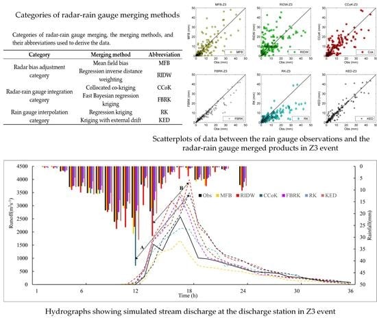
2.1. Radar-Rain Gauge Merging Methods

The potential of high spatial and temporal resolution precipitation based on weather radar is known. Hence, different merging methods have been proposed, and are generally classified as bias reduction and error variance minimization [33]. Identifying the spatial correlation in the error structure model is the most important step in the merging process. A categorization similar to a starting point and refined based upon a theoretical categorization was adopted by Wang et al. (2013), who also proposed the following (

Table 1. Categories of radar-rain gauge merging, the merging methods, and their abbreviations used to derive the data.

Category	Merging Method	Abbreviation
Radar bias adjustment category	Mean field bias	MFB
	Regression inverse distance weighting	RIDW
Radar-rain gauge integration category	Collocated co-kriging	CCoK
	Fast Bayesian regression kriging	FBRK
Rain gauge interpolation category	Regression kriging	RK
	Kriging with external drift	KED

): First, a radar bias adjustment methods focusing on bias adjustment of radar estimates; second, radar-rain gauge integration methods, undertaking a true integration of both radar precipitation and rain gauge data; and, third, rain gauge interpolation methods using different interpolation methods with the radar spatial association as additional information [21].

2.1.1. Radar Bias Adjustment Category

The methods in this category attempt to predict the ungauged location value by the bias that computes radar accumulation and the rain gauge accumulation. In this category, the rain gauge observation is assumed as the true rainfall value, the radar precipitation is used as the entire background, and the radar values at the gauged locations are used to compare with the bias adjustment [34,35]. The ungauged locations value is adjusted by multiplying or adding the gauge-radar comparison correction factor, which is given over a long or short time period [36].

(1) Mean field bias QPE (MFB)

Mean field bias (MFB) adjustment is the simplest method in this category and assumes that the radar estimates are affected by a spatially uniform multiplicative error, which can be a bad electronic calibration or an offset in the Z-R relation used to convert radar reflectivity to rainfall value [13,34]. It is acknowledged that MFB adjustment is the most common and simplest technique in radar meteorology and the correction factor is simply obtained by comparing a spatially averaged ratio of rain gauge with the radar accumulations at gauged locations over the given time period. In this method, a simple multiplicative factor is used to correct the radar domain uniformly. In the current study, the adjustment factor is estimated as

$$C_{MFB}=\frac{{\sum }_{i=1}^N{G}_i}{{\sum }_{i=1}^N{R}_i}$$

(1)

where $N$ is the number of valid rain gauge, $G_i$ is the rain gauge observations, and $R_i$ is the radar estimated values at the rain gauge located pixel.

(2) Regression inverse distance weighting (RIDW)

In this method, the rain gauge observations are used as the true rainfall value to correct the entire radar background field by multiplying a dynamic adjustment correction factor. In geostatistics, a random process R(s, t) consists of two parts, where the first deterministic part D(s, t) corresponds to the trend component, and the other stochastic residual part ε(s, t) corresponds to local fluctuations of the trend. In this study, in addition to the observation vector g(s, t) measured by the rain gauge, the radar-based QPE at rain gauge locations over the whole period were also considered and used at each interpolation point. In this context, the radar external variable was used as a linear function to model the trend D(s, t) [23], so that

$$\mathrm{R}\left(s,t\right)=D\left(s,t\right)+\epsilon \left(s,t\right)$$

(2)

$$\mathrm{D}\left(s,t\right)=a\left(t\right)r\left(s,t\right)$$

(3)

where s is the location of a given point at time t. $r\left(s,t\right)$ is the radar value at location s and time t. The coefficient is computed as the slope of a linear regression of all pairs of points composed of the gauge values on the y-axis and the values of the radar pixel on the x-axis. $a\left(t\right)$ is assumed to be constant spatially.

$$\epsilon \left(s,t\right)=\mathrm{g}\left(s,t\right)-D\left(s,t\right)=g\left(s,t\right)-a\left(t\right)r\left(s,t\right)$$

(4)

$${\widehat{R}}_{RIDW}\left(s,t\right)=D_p\left(s,t\right)+{\widehat{\epsilon }}_{RIDW}$$

(5)

2.1.2. Radar-Rain Gauge Integration Category

The methods in this category aim to minimize the estimation uncertainty by conducting an actual integration of both rain gauge and radar data. As well as differing with some local bias adjustment aiming at reducing local biases between radar and rain gauge observation, the integration category also attempts to minimize overall estimation uncertainty [22]. The merging methods in this category do not simply retain the radar as background or impact the local magnitude at the rain gauge location, but depend on their relative uncertainties and estimate the rainfall value at given location grid in the weighted average of both resources [37]. Two main methods in this category are applied to obtain a minimum uncertainty estimation in different ways, which are:

(1) Collocated co-kriging (CCoK)

To achieve the final aim of reducing uncertainty as much as possible, this method integrates both data instead of using only radar or rain gauge precipitation as the background. The co-kriging (CoK) belongs to this category because it minimizes the variance of estimation by solving a single kriging system, including both radar and rain gauge data. Although CoK can be seen as a radar-based interpolation, it is a liner combination of a multivariate variant, merging radar and rain gauge data [38]. These results, however, from several full forms of CoK with different secondary variables, show a significantly larger kriging system and always lead to a numerically unstable co-kriging matrix, with a significant difference between the primary and secondary data. To avoid these uncertainties, collocated co-kriging (CCoK) has been proposed as a reduced form of CoK and applied in merging rainfall with this variation [39,40]. Compared with CoK, CCoK employs the radar value at the rain gauge location and only incorporates the cross-covariance between the radar value and observation at the rain gauge location. Consequently, the kriging system has been efficiently reduced.

The CCoK estimates rainfall and can be defined as

$$R_{CCoK}\left(s_0,t\right)={{\displaystyle \sum }}_{i=1}^n{\lambda }_i^{CCoK}{R}_g\left(s_i,t\right)+{\lambda }_2^{\prime }{R}_r\left(s_0,t\right)$$

(6)

where $R_g\left(s_i,t\right)$ are the rainfall values of the n known rain gauges at time t, ${\lambda }_i^{CCoK}$ are the weights of the rain gauges, $R_r\left(s_0,t\right)$ is the radar QPE value at the target point, and ${\lambda }_2^{\prime }$ is the weight of related to the radar field.

In this method, the constraint of both data weight can be defined as

$${{\displaystyle \sum }}_{i=1}^n{\lambda }_i^{CCoK}+{\lambda }_2^{\prime }=1$$

(7)

The full radar covariance is, hence, not required. Instead, the covariance of rain gauges and the cross-covariance between radar and gauges are necessary. In this paper, we used rain gauge data and radar data as the primary variable and the secondary variable, respectively, to integrate the precipitation estimation, and approximate the cross-correlation from the radar spatial correlation using the alternative Markov approach [41]. Instead of the multiple (cross-) spatial correlation and large equations using the full COK, for this study, the CCoK used a simplified approximation with its advantage easily applied [40].

$${{\displaystyle \sum }}_{i=1}^n{\lambda }_i^{CCoK}{C}_{GG}\left(x_i,x_0\right)+{\lambda }_2^{\prime }{C}_{GR}\left(x_i,x_o\right)=C_{GG}\left(x_i,x_o\right)$$

(8)

$${{\displaystyle \sum }}_{i=1}^n{\lambda }_{ki}^{CCoK}{C}_{RG}\left(x_0,x_i\right)+{\lambda }_2^{\prime }{C}_{RR}\left(0\right)=C_{RG}\left(0\right)$$

(9)

where $C_{GG}\left(h\right)$ is the covariance of the rain gauges, $C_{RG}\left(h\right)$ is the cross-covariance between radar and rain gauges, and $C_{RR}\left(0\right)$ is the radar covariance at h = 0.

(2) Fast Bayesian regression kriging (FBRK)

In this category, we integrated both rainfall data with the purpose of obtaining the estimation at the minimum uncertainty. For this purpose, methods in a Bayesian framework are widely used, and we applied the fast Bayesian regression kriging (FBRK), method, as proposed by Yang and Ng [42], to merge different data types [42]. We explicitly considered the difference in the errors from the raw input data and aimed to estimate an accurate rainfall field and obtain better precipitation data. Unlike most other existing kriging-based merging methods, the likelihood function in the FBRK is modified. Further accounting for the differences, Yang and Ng [42] applied the FBRK in three different data types, i.e., the residuals of the regression model were used to regress radar estimations, and rain gauge observations were interpolated by the ordinary kriging.

$${\widehat{I}}_0=a_r{R}_0+{\beta }_r+e_0$$

(10)

where ${\hat{I}}_0$ is the FBRK interpolated rainfall intensity at $x_0$, $R_0$ is the radar measured intensity at the same location, $a_r$ and ${\beta }_r$ are the regression coefficients, and $e_0$ is a random error term whose mean and standard deviation are computed following the kriging equations below:

$$u_{e0}={{\displaystyle \sum }}_{i=1}^M{\lambda }_i{e}_i$$

(11)

$${\sigma }_o^2=\left(1-{{\displaystyle \sum }}_{i=1}^M{\lambda }_i\right){\gamma }_{\infty }+{{\displaystyle \sum }}_{i=1}^M{\lambda }_i{r}_{0,i}$$

(12)

$$r_{i,j}={\tau }^2+s^2\left[1-exp\left(-\frac{\left|x_i,x_j\right|}{d_{\infty }}\right)\right]$$

(13)

$$\left(\begin{array}{ccc}{r}_{1,1}& \cdots & r_{M,1}\\ ⋮& \ddots & ⋮\\ r_{1,M}& \dots & r_{M,M}\end{array}\right)\left(\begin{array}{c}{\lambda }_1\\ ⋮\\ {\lambda }_M\end{array}\right)=\left(\begin{array}{c}{r}_{0,1}\\ ⋮\\ r_{0,M}\end{array}\right)$$

(14)

where $u_{e0}$ and ${\sigma }_o$ are the expected value and standard deviation of $e_0$, respectively, $e_i$ is the residual of the ith of the M rain gauge and crowdsourced observations, and ${\lambda }_i$ is its associated weight.

2.1.3. Rain Gauge Interpolation Category Using the Spatial Association of Radar as an Addition

Unlike the bias adjustment methods using the entire radar field as background with these integration methods integrating both data sources, the methods in this category simply used the spatial association as an external drift to interpolate the rain gauge values. Ochoa-Rodriguez et al. proposed that the merging methods in this category are all geostatistical and kriging-based [33]. The kriging-based interpolation approaches predict the ungauged located values with the linear weights of observations at gauged locations by minimizing the variance of the error. As such, the main component of the methods is that the rainfall filed can be characterized as a Gaussian random variable, and because of this, the methods predict ungauged values with the liner combination of gauged value by deriving the weights through minimizing the variance. This differs to the classical geostatistics by assuming a Gaussian distribution and stationarity of the spatial covariance, with the distribution of precipitation skewed over the domain [43]. The transformation of applying both rain gauge and radar data into a more Gaussian distribution is termed trans-gaussian kriging [44]. It is based on the quantitative spatial variability of both data, and a more Gaussian distribution always has a better Gaussianity in the residuals. Two widely used methods of this category were applied in this study, which are:

(1) Regression kriging (RK)

As one of the kriging family hybrid interpolation methods, regression kriging (RK) is a spatial interpolation technique that integrates a linear regression and the regression residuals with simple kriging. The advantage of this method is that all points are used to interpolate the residual with a global neighborhood, which can extend to a broader range. RK uses arbitrarily complex regression on auxiliary information (radar data) and chooses simple kriging to interpolate the residuals acquired from the regression model. In this study, we defined the following successive steps to implement this method: (a) The linear regression step, (b) the residuals variogram computation step, and (c) the kriging-based interpolation of the residual steps.

For steps a and b, the trend and residuals computation based on Equation (3) are also valid for RK. At the beginning of step c, the covariance matrix $C_{aa}$ of computing the covariance of the residuals at the target location is:

$$C_{aa}=\left(\begin{array}{cc}\begin{array}{cc}{C}_Z^2& C_{12}\\ C_{21}& C_Z^2\end{array}& \begin{array}{cc}\cdots & C_{1N}\\ \cdots & C_{2N}\end{array}\\ \begin{array}{cc}⋮& ⋮\\ C_{N2}& C_{N2}\end{array}& \begin{array}{cc}\ddots & ⋮\\ \cdots & C_Z^2\end{array}\end{array}\right)$$

(15)

where element $C_{aa}$ of the matrix is computed by the covariance between the observation locations I and j, where $C_Z^2$ is the variance of the observations. In this method, the square-root transformation of the data is used in the process of applying kriging. This transformation shows a trending increase on the Gaussianity of the overall residuals, although some analysis of the effect sometimes show a few that are limited. Based on the linear kriging and linear combination, the weights used to compute residuals at the target location could thus be given as:

$${\widehat{ϵ}}_{RK}\left(s_0,t\right)={{\displaystyle \sum }}_{i=1}^N{\lambda }_i\in \left(s,t\right)$$

(16)

which is then added to the trend $m_p\left(S_0,t\right)$ to obtain the expected value of the precipitation depth.

Finally, the expected precipitation value at the interpolation location can be computed as:

$${\widehat{p}}_{RK}\left(s_o,t\right)=m_p\left(s_0,t\right)+{\widehat{ϵ}}_{RK}\left(s_0,t\right)$$

(17)

(2) Kriging with external drift (KED)

Kriging with external drift (KED) is an extension of universal kriging interpolation, in which the interpolated variable, in this case, is computed as the sum of stochastic term and a deterministic term. Kriging with external drifts allows the incorporation of several additional variables that are used as background information to interpolate the primary variable [45]. In this study, we focused on merging rain gauge and radar data, and therefore, radar data were considered as the only additional information in this method. The basic assumption of KED is that the expected value of the estimated variable $\mathrm{G}\left(x\right)$ has a linear relationship with an additional variable $R\left(x\right)$:

$$\mathrm{G}\left(x\right)=a+b\cdot R\left(x\right)$$

(18)

where $\mathrm{G}\left(x\right)$ is the rain gauge value at location x, $R\left(x\right)$ is the radar rainfall estimate at the gauged location x, and a and b are linear coefficients that are determined.

The external drift can clearly indicate the full spatial variability of the radar QPE data, especially in the events that the rain gauge-radar consistency is high. Thus, the estimation at given location x₀ is derived from a linear estimator, and the weights are computed as follows:

$${{\displaystyle \sum }}_{i=1}^n{\lambda }_i^{KED}=1$$

(19)

$${{\displaystyle \sum }}_{i=1}^n{\lambda }_i^{KED}R(x_i)=R(x_0)$$

(20)

As mentioned above, data transformation is used to deal with the rainfall showing non-Gaussian features and the problematic cases that lack enough rain gauges to obtain a reliable variogram [46]. In this method, normal score transformation, which can associate every given probability quantile to the corresponding quantiles of a standard normal probability distribution, is used to transform the data to obtain a continuous, strictly cumulative distribution [44].

2.2. Meteorological Evaluation

2.2.1. Leave-One-Out Cross Validation (LOOCV)

No independent precipitation observations exist at a high resolution. Hence, to validate the merging methods, a leave-one-out cross validation (LOOCV) was used to assess the performance of the rainfall-merged techniques. In this method, the rain gauge point observations are assumed to be directly measured as true values, which are used to access the performance by a comparison with other given grid point rainfall products that are computed by different rainfall-merged methods. For the scale mismatch between rain gauge and merging grid cell, the gauged location value is substituted by merged rainfall data from the nearest grid center. It is notable that LOOCV only assesses the accuracy of estimations at the rain gauge locations, but the LOOCV statistics allow us to compare the performance of different merging methods systematically.

In this study, we undertook the evaluation on an hourly basis for each rain gauge location and for each of the merging methods.

The following indicators were used to quantitatively compare the different radar-rain gauge merged products and the rain gauge observations for each time step:

Bias: The systematic errors assessment is calculated from the mean of difference between the observed and predicted rainfall values.

$$\mathrm{Bias}=\frac{1}{n}{{\displaystyle \sum }}_{i=1}^n\left(R_i-{\widehat{R}}_i\right)$$

(21)

RMSE: The root mean square (RMSE) represents the standard deviation of the differences between the observed and predicted rainfall values and is widely used in verification.

$$\mathrm{RMSE}=\sqrt{\frac{1}{n}{{\displaystyle \sum }}_{i=1}^n{\left(R_i-{\widehat{R}}_i\right)}^2}$$

(22)

MRTE: The mean-root-transformed error (MRTE) can mitigate the dominant of errors from large precipitation amounts for the given lower weight:

$$\mathrm{MRTE}=\frac{1}{n}{{\displaystyle \sum }}_{i=1}^n{\left(\sqrt{R_i}-\sqrt{{\widehat{R}}_i}\right)}^2$$

(23)

where $R_i$ is the rain gauge observed value, n is the number of the rain gauges, and ${\widehat{R}}_i$ is the estimated value at the rain gauge location. For each whole event, the bias was computed as an average of the entire period and entire spatial range. The bias value can range from −∞ to +∞, with optimal value equal to 0. The RMSE and MRTE can range from 0 to +∞, with optimal value equal to 0.

Finally, the assessment of individual rain gauges only provides a performance at the point scale. For the catchment that has fewer rain gauges to validate the performance, the evaluation over the whole catchment is necessary. Thus, in order to assess the performance of the merging methods at larger areas, a hydrological application approach was implemented.

2.2.2. Hybrid Hydrological Model (Hybrid-Hebei Model)

In this study, all the rainfall runoff forecasts were produced with the semi-distributed rainfall-runoff Hybrid-Hebei model. This model is a semi-distributed model with a lumped conceptual from the Hebei model and a spatially distributed feature based on GIS [47]. The model is in operational use in semi-arid and semi-humid regions. The runoff of the semi-distributed Hebei model is divided into surface runoff and underground runoff in each 1-km² grid cell. When the precipitation intensity is greater than the infiltration intensity, the landmark runoff confluence is generated and, conversely, the infiltration component generates underground runoff after considering the soil water demand. Finally the confluence generates the outlet flow of the basin. The structure of the Hebei model in each 1-km² grid cell is shown in Figure 1.

In semi-humid and semi-arid areas, the middle zone of the soil vadose zone is relatively thick, the infiltration rate generated by precipitation often fails to reach the diving surface, and the infiltration rate gradually decreases during the infiltration process. Therefore, the main factor affecting the infiltration rate is the water content of the surface soil. In the semi-distributed Hebei model, considering the complex changes of the underlying surface and the significant difference in infiltration capacity in the semi-arid and semi-humid areas, the infiltration curve in the model is a parabolic infiltration curve controlled by surface soil moisture. This is based on measured data of the Tuanshan gully in northern Shaanxi, China.

The model’s infiltration curve within the grid is:

$$f_g=\left(p_g-\frac{i^{\left(1+n\right)}}{\left(1+n\right)f_m^n}\right)e^{-um}+f_c$$

(24)

where $f_g$ is infiltration rate within the grid, unit: mm/h; $p_g$ is rainfall intensity within the grid, mm/h; n is the index; $f_c$ is stable infiltration rate, mm/h; u is the index; m is the surface soil moisture, mm; and $f_m^n$ is the infiltration capacity within the grid, mm/h.

The structure of the lumped Hebei model was described in a previous study [47]. Compared to the original lumped Hebei model, the Hybrid-Hebei model provides improved hydrograph simulations. It can be coupled with high-resolution precipitation to achieve a superior runoff simulation. In this study, the Nash efficiency coefficient (NSE) was used to evaluate the ensemble runoff simulation.

$$\mathrm{NSE}=1-\frac{{\sum }_{t=1}^T{\left(Q_0^t-Q_m^t\right)}^2}{{\sum }_{t=1}^T{\left(Q_0^t-{\overline{Q}}_o\right)}^2}$$

(25)

where $Q_0^t$ is the observation at time t, $Q_m^t$ is the estimated value at time t, and ${\widehat{Q}}_o$ is the mean value of the whole time T.

For floods in mountainous catchments, the peak flow is an important index, and the relative error (RE) of the peak flow is adopted:

$$\mathrm{RE}=\frac{Q_m-Q_p}{Q_p}$$

(26)

where $Q_p$ is the observed peak flow and $Q_m$ is the estimated peak flow.

3. Study Area and Data

3.1. Study Area and Events

The two river catchments of Fuping and Zijinguan were selected as the study areas. These catchments belong to the south and north reaches of the Daqinghe catchment located in Northern China and have semi-humid and semi-arid climatic conditions. The drainage area of Fuping (from latitude 39°22′ to latitude 38°47′N and from longitude 113°40′ to longitude 114°18′E) is 2210 km², and the area of Zijingguan (from latitude 39°13′ to latitude 39°40′N and from longitude 114°28′ to longitude 115°11′E) is 1760 km². The elevation above sea level in the Fuping and Zijingguan catchments varies from 254 m to approximately 2456 m and 519 m to 2105 m, respectively (Figure 2). Both catchments react very specifically to intense rainfall for the steep terrain and the low vegetation coverage, and the rivers of the two catchments flow from west to east. The river flow is measured at the catchment outlets. There are eight rain gauges in the Fuping catchment and eleven rain gauges in the Zijingguan catchment. An S-band Doppler weather radar with a scan radius of 250 km is located in Shijiazhuang city, which is approximately 100 km to the southeast of the two catchments and both catchments can be completely covered by the radar. In this study, four storm events from the Zijingguan catchment and four storm events from the Fuping catchment were selected to assess the performance of different merging methods. When we chose the storm events, a 24-h time window was used. Within the 24-h window, the storms which showed representative rainfall evenness in space and time were chosen, which then formed the eight storm events. The start times, durations, and peak flows of these events are shown in

Table 2. Durations and rainfall totals for the eight selected storm events.

Catchment	Event ID	Date	Start Time	Duration	Rain Gauges	Accumulated Rainfall (mm)	Peak Flow (m3s−1)
Zijingguan	Z1	22/05/2007	00:00	17 h	11	39.52	6.8
	Z2	10/08/2008	00:00	10 h		45.53	2.5
	Z3	21/07/2012	04:00	14 h		155.43	2580.0
	Z4	19/07/2016	05:00	19 h		74.29	53.4
Fuping	F1	29/07/2007	20:00	24 h	8	63.38	29.7
	F2	30/07/2012	08:00	24 h		50.48	70.7
	F3	01/09/2012	08:00	18 h		40.30	13.7
	F4	25/07/2016	00:00	11 h		10.8	2020

.

3.2. Weather Radar and Data

The radar data used in this study were retrieved from the S-band single-polarization Doppler weather radar located at Shijiazhuang city in Northern China (Figure 1). The detailed information of this radar can be seen in

Table 3. The parameters and hardware functions of the Shijiazhuang SA Doppler Radar.

Radar Name	Name of Radar Site	Frequency (GHz)	Beam Width (°)	Antenna Diameter (m)	Pulse Width (μs)	Antenna Gain (db)	Peak Power (kw)
Shijiazhuang	SA	2.7~3.0	1	11.8 *	1.57	≥44	650

* The antenna diameter includes the radome.

. The radar is operated by the China Meteorological Administration (CMA) and has an optimal detection range of 230 km. The radar obtains per base reflectivity data on every six-minute volume scan and completely covers the two study areas [48]. A radar QPE Group System (QPEGS) was developed by the CMA, providing hourly QPE data at a high spatial resolution. For different sources of errors, such as radar calibration, variation of the vertical reflectivity profile, attenuation, and anomalies, quality control of radar data, such as the removal of ground clutter, is necessary and carried out by the OPEGS. A maximum-pixel-value method was also used to generate the “mixed height radar reflectivity” in each volume gridded value, as in the hybrid scan reflectivity proposed by the National Severe Storms Laboratory (NSSL). For the location of the selected radar in this study, a threshold value (38 dBZ) of radar reflectivity was set to differentiate between the convective and stratiform rainfall types considering the rainfall features in eastern China [49]. The accumulated clutter was always magnified during the hourly accumulated rainfall collection period, so a simple clutter filter was used to remove the static clutter. The power law Marshall–Palmer relationship converted the radar reflectivity (Z) to rain rata (R), and a Z-R relationship calculated the accumulated rainfall for convective and stratiform rainfall types [50]. In the QPEGS, the common definition of “a” and “b” is shown in Equations (25) and (26) [48]. To ensure that the spatial resolution of radar data can reflect the precipitation, a higher radar precipitation, rather than a low threshold of 0.1 mm, was considered for the estimation of a 1 km × 1 km radar grid.

For convective:

$$\mathrm{Z}=300R^{1.4}$$

(27)

For stratiform:

$$\mathrm{Z}=200R^{1.6}$$

(28)

4. Results and Discussion

We produced a series of sets of radar-rain gauge merged data by combining the radar and rain gauge precipitation using different merging methods. During the computing period with these merging methods, some applications were defined. For example, a value of 2 (common default value) was given in the RIDW method, and a minimum of three stations were used in the kriging-based methods. Spherical-model semivariograms defined the variograms that were ill defined, with an insufficient number of points. The last previously computed valid variogram was instead used when the present condition was not valid, and the regression and integration were computed on stations only located in the basins [51,52]. The evaluation of the quality and the reliability of the merged data in this study was assessed in two stages: The quantitative evaluation of radar-rain gauge merging methods based on LOOCV and the hydrological model performance driven from the merged data as Hybrid-Hebei model input.

4.1. Evaluation of Radar-Rain Gauge Merging Methods

To assess the performance of the different merging methods, we computed the present performance indicators for the eight events. For each indicator, hourly rainfall values were averaged for each event (

Table 4. The indicators performance based on leave-one-out cross validation (LOOCV) in the two catchments.

Basin	Indicator	OR	MFB	RIDW	CCoK	FBRK	RK	KED
Zijingguan	BIAS	−2.84	−1.69	1.61	0.58	0.24	−0.71	0.34
	RMSE	4.84	4.49	3.28	3.3	1.31	2.92	1.41
	MRTE	1.86	1.22	1.03	0.55	0.21	0.78	0.22
Fuping	BIAS	−1.08	−0.36	0.33	0.20	−0.08	−0.28	−0.11
	RMSE	3.78	2.14	1.64	2.22	1.18	2.72	1.21
	MRTE	1.63	0.98	0.49	0.57	0.19	0.73	0.22

, Figure 3), and the calculated weight of each rain gauge was determined by the area weight divided by the Thiessen polygon. As indicated, the QPE-only-based radar data (OR) clearly showed the weakest performance in all performance indicators, which confirms the necessity of bias correction using rain gauge observations. For the BIAS indicator, the median of BIAS should be close to zero with minimum dispersion because the cross-validation errors of a good estimator should be unbiased. The results shown in Figure 3 indicate that all merging methods were relatively unbiased (median errors were close to zero in all events), but the range of BIAS varied between the different methods. The main difference between these methods can be seen in the range of the indicators, whereby the integration category has the smallest range of BIAS rather than the interpolation category and bias adjustment category [53]. The results show that the kriging-based methods all performed well, with the bias reduced. A comparison of the results of the three categories on the RMSE and MRTE (Figure 3) is noticeable. Irrespective of the two merging methods chosen in the integration or interpolation category, one of these had a clear improvement over the bias adjustment and another has a slight improvement. The performance and added value of the associated merging methods generally increase with the improvement of correlation between rain gauge and radar estimation for medium or large geographic domains, but is invisible for the smaller domains for the limited rain gauges observation and the uncertainty of precipitation under rapid spatial transformation [33].

Figure 3 provides a graphical representation of the results of the different merging methods on the two basins and indicates that the FBRK results performed best, followed by the KED, CCoK, RK, RIDW, and MFB. The improvement of the FBRK data over the KED, however, was relatively minor compared to their improvements over other merging methods. The two methods that performed best were the FBRK and KED, which belong to the integration category and interpolation category, respectively. It has been pointed out in previous studies that the methods in the bias adjustment category were not found to have a better performance in any inter-comparison studies [32,54]. The results of these methods make us consider that correction can be used to estimate all points inside the study area and can deal with anisotropy and the spatial evolution of precipitation with assuming translation invariance and small basins. The results are not clear, however, for partial methods and indicators. For example, the RIDW performed better overall than the CCoK and RK when applied in Fuping. In terms of the BIAS, the RIDW showed a similar performance with the FBRK or KED and had a better performance than CCoK or RK in terms of RMSE and MTRE indicators. This is due to the fact that the quality of the kriging-based methods and bias adjustment methods depend significantly on the geometry of the rain gauge network distribution and, in particular, on the low-density rain gauge network [32].

Through the overall comparison of the performance of the two basins using different merging methods, we found that different merging methods not only produced similar results, but also showed different performances. This is because there is an information gap, such as the area of the basin, the distribution information of the rain gauges, and the distance from the radar. Therefore, we need to analyze and discuss each basin in order to determine suitable merging methods that suit different basins and the reasons for their suitability, as well as the reasons why other methods do not perform well.

In

Table 5. The indicator performance based on LOOCV in Zijingguan.

Event	Indicator	OR	MFB	RIDW	CCoK	FBRK	RK	KED
Z1	BIAS	−0.84	−0.49	0.25	0.12	0.07	−0.16	−0.10
	RMSE	2.33	1.05	1.08	0.87	0.41	1.05	0.53
	MRTE	0.73	0.34	0.23	0.16	0.04	0.18	0.06
Z2	BIAS	−1.195	−0.78	0.61	−0.14	−0.06	−0.31	0.09
	RMSE	5.69	2.26	2.15	1.86	0.85	1.97	1.07
	MRTE	1.87	0.67	0.52	0.34	0.09	0.40	0.14
Z3	BIAS	−4.40	−2.36	2.34	1.17	0.54	−1.01	0.76
	RMSE	9.11	7.97	5.35	6.17	2.96	5.78	3.23
	MRTE	2.69	1.90	1.27	1.53	0.50	1.34	0.69
Z4	BIAS	−2.68	−1.01	0.71	−0.33	−0.16	−0.66	0.21
	RMSE	6.61	4.12	3.12	1.31	0.97	2.10	0.99
	MRTE	2.12	1.68	1.11	0.66	0.20	0.87	0.31

, the indicator performances of the merging methods for the four storm events of Zijingguan are shown. Figure 4 and Figure 5 show the boxplot of the three indicators for the four events in different merging methods and the scatterplot of the rain gauge observations with the predicted rainfall values from the six merging methods. The merging methods generally outperformed the radar-only estimations and the quality of radar data determined the quality of the merging products. The BIAS shows a clear underestimation when comparing the radar QPE with the rain gauge observation and confirms the need for correction of the radar QPE using rain gauges. The results for the BIAS show that for the performance of the rainfall data compared with the gauge observation, OR and MFB showed a strong negative value and the RIDW had a strong positive value. The other methods had a bias value of approximately 0. Furthermore, the values of the RMSE and MRTE strengthen the observation. It can also be seen that the interpolation methods and integration methods performed better than the bias adjustment methods. This could be due to the simplicity of bias adjustment methods and the complex formulation of the other two methods. It seems that a more complex implementation of merging methods always achieves a better result.

The FBRK method and the KED method provided the best performance and second-best performance, respectively, for the three indicators, whereby they provided the best and second-best values over all four events in the Zijingguan catchment. The scatter diagram (Figure 5) demonstrates that the FBRK and KED had a significant relationship between the merging data and rain gauge data, thereby indicating the high potential of merging skills in the applications. To the authors’ knowledge, in all merging methods studied, the BAY-based method and the KED are the most popular merging methods that generally perform best [32], and this is in concordance with our results. The overall indicators and events show that the FBRK has a slightly better performance than KED. The third and fourth best performing methods were the CCoK and the RK methods. It is noted that the BIAS value-based RK had a slightly negative bias. In terms of all indicators, CCoK outperformed for three events, but for the Z3 event, the RK performed better than CCoK. The RK preserved the relative spatial rainfall resolution of the radar data, but its value estimates tended to be under the range of the gauge observations. We highlight that the RIDW method was applied with the default value of 2 [52]. The parameter, however, is often applied across large areas (particularly including a degree of spatial varying of rain gauge-radar biases), along with small-scale features that are spatially variable. This means that a default value may fail to quantitatively correct the rainfall data. An adjustment of the parameter may achieve a better performance of the RIDW method. The MFB performed worst in all methods and events. The MFB is, however, the most commonly used and investigated method among all merging methods, and it scales the original radar data to match the rainfall accumulations recorded by rain gauges. Considering this, the MFB can potentially provide a better representation of small-rainfall features compared with the other five merging methods [33]. The simple use and way in which the radar QPE is employed throughout the merging process, however, suggests that the MFB may fail to satisfactorily correct the rainfall features.

Table 6. The indicator performance based on LOOCV in Fuping.

Event	Indicator	OR	MFB	RIDW	CCoK	FBRK	RK	KED
F1	BIAS	−1.87	−0.93	0.41	0.76	−0.23	−0.68	−0.31
	RMSE	5.43	3.33	2.35	2.12	1.42	2.67	1.66
	MRTE	3.27	1.40	1.06	0.73	0.19	1.28	0.43
F2	BIAS	−0.93	−0.53	0.17	0.21	0.08	−0.24	0.09
	RMSE	2.79	1.89	1.36	1.84	0.61	1.45	0.96
	MRTE	1.55	0.62	0.33	0.45	0.11	0.34	0.20
F3	BIAS	−0.95	−0.53	0.21	0.26	0.03	−0.26	0.07
	RMSE	2.71	1.32	0.89	1.01	0.51	0.92	0.65
	MRTE	0.71	0.47	0.18	0.28	0.06	0.19	0.12
F4	BIAS	−0.59	−0.25	0.17	0.24	−0.04	0.28	0.05
	RMSE	4.18	2.02	1.68	1.87	0.43	1.78	0.64
	MRTE	0.88	0.36	0.21	0.26	0.06	0.26	0.11

shows the indicator performances of the merging methods for the four storm events of Fuping. Figure 6 and Figure 7 show detailed information regarding the six merging methods applied in Fuping. The results of the performances for the three categories are the same as those of the Zijingguan events. When comparing the indicator performances of the two basins, the OR performed better in Fuping, inferring that there was a better QPE for close to the radar station. As expected, the methods belonging to the bias adjustment category had a better performance than their applications in Zijingguan. In contrast to the results of the chosen methods applied in Zijingguan, it is clear that the RIDW belonging to the bias adjustment category outperformed the CCoK belonging to the integration category and the RK belonging to the interpolation category. It is well known that the smaller the value in the indicators and the smaller the range in the boxplot, the better the scatter correction. The better QPE is the main reason leading to the superior performance of the RIDW, and with a better QPE, the RIDW can preserve the original structure of the radar rainfall, especially the small-scale features. The RK method is highly reliant upon rain gauge numbers because it simply utilizes the spatial information of the radar field at the rain gauge locations to interpolate. As well as the ability of RK to reproduce rainfall features, it is highly dependent upon the density of rain gauges at the small scale. The RK method is likely to be used more in the limited rain gauges, with the variogram generation based on the point rain gauge value. The relatively poor performance of the CCoK and RK results (Figure 6) were likely due to the assumption that the Gaussian distribution in dynamic merging methods would compute results that may be limited in simulating rainfall values [43]. For CCoK, the method takes spatial information from the radar in the basin. According to the performance results (Table 6), the better QPE and limited rain gauges combined to produce a satisfactory performance.

Through the comparison of the three evaluation indicators with the two basins, the two classical approaches (FBRK and KED), based on inotropic and variograms, are the best suited of the merging methods, which work well with the high spatial and temporal variability of precipitation. The performance of the different merging methods is clearly shown in this section. Multiple factors, which affect the application of radar-rain gauge merging methods used in the basins, were identified in this study. Obviously, the most important single factor affecting the performance is the quality of QPE that indicates the ability of radar to sample the rainfall conditions [55]. As the application in the Fuping shows, the RIDW, based a better QPE, outperformed the CCoK and RK, although the limited rain gauges significantly affected the performances of these methods. The lack of rain gauges created a lack of consistency provided by radar and rain gauges. As some studies have found, merging performance generally improves with increasing consistency between radar and rain gauge measurements, particularly in the integration and interpolation categories [19].

For small-scale basins, the preservation of small-scale rainfall features is critical to apply the methods. Different merging methods mean different choices regarding how the radar and rain gauge data are treated and applied during the merging process [56]. In this study, methodological choices focused on improving the quality of radar and rain gauge estimates through different methods. For small-scale basins, the radar QPE was the main data source, providing spatial details of the rainfall. Thus, the ability of these merging methods to preserve local rainfall features was highly dependent on the proportion of, and way of, employing radar data through the merging process. As described in Section 2.1.1, the bias adjustment category scaled the original radar estimation by multiplying the QPE accumulations with factors to match the rain gauge record. As such, the original structure of the radar rainfall field was essentially preserved. However, the MFB did not achieve a satisfactory performance in the rainfall rates correction associated with small-scale features. Because MFB is usually applied uniformly to large areas, it often ignores the spatial variability in radar QPEs when applied at the small scale [57]. As Table 6 demonstrates, RIDW achieved a satisfactory performance with a high-quality radar QPE. As discussed in the previous section, a local regression of the radar data on the rain gauge data could contribute positively to the RIDW performance. The methods in the integration category combine the two datasets based on their relative uncertainty (see Section 2.1.2). As such, with limited rain gauges or high spatial rainfall variability, integration methods take more information from the radar data. This means that it is possible for integration methods to obtain a satisfactory reproduction of small-scale features, as in the assessment result of FBRK (Table 5). To a certain extent, however, CCoK prefers the interpolation category, in both the performance of comparison from the results and the Gaussian assumption. Unlike the other two categories, the methods in the interpolation category are highly reliant on rain gauge observations, simply considering the gauged radar data in the interpolation process. As per the result comparison discussed in the previous sections, the performance of interpolation-based methods is clearly associated with the density of rain gauges, which decide the ability to capture the small-scale rainfall features. Conversely, interpolation methods with Gaussian assumptions always smooth the high nonlinearities in small-scale features [58]. This is why the error of the RK prediction value is more obvious when the precipitation is large. For KED, the spatial details are reconstructed after the merging process. The density of rain gauges employed in radar-rain gauge merging has an impact on the performance of the merging methods. The impact of limited rain gauge availability on merging performance is closely linked to the reliance of a given merging method upon rain gauge data, as well as to the way in which radar data is employed in the merging process. Having a sufficient number of rain gauges in the study area may increase the ability of the rain gauges to capture the relevant precipitation features. However, the two catchments in this manuscript had a limited number of rain gauges due to the lack of monitoring network. With the increasing of monitoring stations, a further work should be implemented to study the influence of the rain gauge density on the merging performance.

In the six chosen merging method performances, we conclude the strengths and weaknesses of the three categories. The bias adjustment category has the advantage of ease of use, which leads to its wide application. For the methods in this category, small-scale rainfall features are generally preserved, although the correction may fail to correct the rain rates. The integration category allows for the consideration of rain gauge and radar uncertainties. The complex computation of the integration category, such as requiring solving matrix systems, leads to it being applied and tested the least. The interpolation category ranks between the other two categories in both complexity and performance, which is why the methods in the interpolation category are becoming increasingly popular [19].

4.2. Hydrological Model Performance Evaluation

The LOOCV analysis result does not allow a direct comparison because the left rain gauge is just used to compare and not used to compute the product [52]. Some authors have proposed that a higher quality of the merging products can be indicated from agreements between the simulated and observed runoff using the merging products as the input [53]. All authors, however, pointed out that the calibration of a hydrological model is a demanding task and subject to various uncertainties, particularly for mountain flood simulations, whereby it is not easy to find the adequate parameters for considering uncertainties in the model structure and parameterization. In this study, a set of calibrated and validated model parameters were, therefore, used with the Hybrid-Hebei rainfall-runoff model in the same two basins [47].

Table 7. The indicator performance based on the Hybrid-Hebei model in two catchments.

Event	Indicator	MFB	RIDW	CCoK	FBRK	RK	KED
Z1	NSE	0.37	0.44	0.51	0.57	0.46	0.60
	RE	−0.47	0.57	0.24	0.21	−0.38	0.26
Z2	NSE	0.47	0.41	0.55	0.59	0.46	0.61
	RE	−0.38	0.33	0.36	0.28	−0.29	0.24
Z3	NSE	0.36	0.52	0.42	0.53	0.41	0.49
	RE	−0.52	0.54	0.35	0.28	−0.16	0.41
Z4	NSE	0.26	0.37	0.41	0.52	0.38	0.50
	RE	−0.68	0.61	0.55	0.38	−0.69	0.28
F1	NSE	0.32	0.38	0.48	0.58	0.42	0.55
	RE	−0.47	0.68	0.56	0.42	−0.48	0.38
F2	NSE	0.41	0.49	0.51	0.61	0.49	0.62
	RE	−0.55	0.95	0.77	0.55	−0.48	0.48
F3	NSE	0.36	0.42	0.46	0.54	0.40	0.51
	RE	−0.49	0.78	0.63	0.37	−0.33	0.65
F4	NSE	0.21	0.38	0.41	0.53	0.35	0.55
	RE	−0.68	0.44	0.36	0.68	−0.57	0.48

shows the performance of merging methods in the runoff simulation. As expected, the merging methods performed a different goodness-of-fit with the runoff simulation. For the NSE, all merging methods performed normally, and the extent of failure was revealed more clearly in RE. The values of NSE were increased from 0.21 (the MFB in F4) to 0.62 (the KED in F2). Concerning peak flows, the values of MFB and RK were negative overall, indicating a general tendency of underestimation together with the performance of rainfall estimates in the previous section. All the other methods showed a higher estimate. It can be noticed that the RK method seemed to have a better performance for the peak flows than FBRK and KED methods for the Z3, F2, F3, and F4 storm events. In this study, the purpose of inputting the QPEs to the hydrological model was not to rank the merging methods, but to test the applicability of the merging rainfall products for flood forecasting. The performance of the rainfall-runoff model is subject to its parameter calibration. Since only one certain set of parameters was used for the Hybrid-Hebei model, the differences of QPEs from different merging methods may be obscured in the runoff simulations. As indicated in Table 7, the MFB performed worse than any of the methods chosen. The best results were the FBRK and KED methods. The performance of the FBRK and KED methods were almost identical when considering the simulation of NSE and RE in the entire events. This may be because the model calibration seems to have compensated for the differences in the rainfall garnering in the merging process. Compared with the CCoK and RK, the CCoK showed a better performance in most events, and therefore, the result indicates that the performance of the hydrological output is highly dependent on the accuracy of the rainfall product. The RIDW method ranked between the RK and MFB in both Fuping and Zijingguan. With one exception (Z3), however, the performances of these merging methods were different from other events.

Figure 8 shows the 24-h accumulated rainfall in the Zijingguan catchment based on different merging methods in the Z3 event. Figure 9 shows the hourly precipitation distribution and simulated stream flow hydrograph of all merging methods in this event, and the hydrograph flood process was extended to 36 h. As indicated in Figure 9, the entire runoff simulation process lines of merging methods had the same trend as the measured flow process line. The runoff hydrograph indicates that the catchment in the study area was relatively fast. The occurrence time of flood peak was the same in all simulation processes, and the peak staggering time was no more than a maximum of one hour. This indicates that the Hybrid-Hebei model can successfully simulate runoff under different precipitation products. For all merging methods, it is can be seen from Table 7 and Figure 9 that FBRK continued to rank highest in the hydrological verification. The RIDW outperformed at NSE because the runoff simulation hydrograph of RIDW was the only one with a double-peak flow as the measured runoff streamline. RIDW, however, was evaluated as only better than the MFB in LOOCV. KED performed the third best in the NSE, however, the extent of failure was found in the peak flow. The CCoK performed worse, and a one-hour peak flow lag was found (Figure 9). RK and MFB both showed an average performance in NSE and RE, and both showed a clear underestimation in peak flow.

Based on the result of NSE (Table 7), the results of runoff simulations were normal. This is particularly because these merging methods do not have a large difference in accumulated precipitation and temporal distribution in Z3 (Figure 9). When considering the peak flow, however, the discrepancy was pronounced in both value and occurrence time. Furthermore, for RIDW and CCoK, the peak flow occurrence time of the other four methods was consistent with the measurement, and the difference between them was the value of peak flow. The lagged phase of the double peak flows in RIDW and peak flow in CCoK was approximately one hour. Compared to line A and line B, clear rainfall random errors in RIDW and CCoK were found, and the response of the runoff model performed differently. It is known that the transformation of precipitation to runoff is a smoothing operation in both space and time. For this catchment, a quick response time leads to a failure in the “smoothing effect.” If the rainfall accumulation is larger than the response time of catchment, the performance of these methods will be improved [53].

In this section, the fitness of the simulated flow driven by different merging products was used to assess the performance of these products. The hydrological performance of the merging methods was not as good as expected. It is notable that, in runoff simulations, these methods all significantly ranked the lowest in the bias adjustment category. This may be because a spatially differentiated correction was not adopted in this category, and the transformation of rain to runoff is a temporal and spatial process. If the correlation length of random errors is close to the catchment’s response time, random errors will be averaged out to a lower extent [53]. For the chosen methods, both FBRK and KED exhibited a low variation of approximately 0.6. The median ranking of RIDW in LOOCV was different to its performance in runoff simulations than CCoK and RK. It should be noted that the potential of giving the merging products as hydrological input is also a function of further multiple factors, including the methodological choices in the merging process, the climatological conditions in the basins, structural model errors, and the cross uncertainties in the entire merging and hydrological application [59]. Moreover, in order to assess the performance of hydrological variables while considering spatial observations, temporal observations must be taken into consideration because products generated by a distributed hydrological model or semi-distributed model, such as stream flow, are found to be sensitive to different high-resolution precipitation [60].

5. Conclusions

In this paper, radar-rain gauge merging categories were conducted. Eight different storm events were chosen from two catchments in semi-humid and semi-arid areas of Northern China to test six different radar-rain gauge-merging methods that belong to three categories using a LOOCV and a rainfall-runoff model (Hybrid-Hebei model). We generated six merged radar-rain gauge rainfall products and compared their performances at gauged location estimations to further their effectiveness as inputs to a semi-distributed rainfall-runoff model of the two study catchments, the Zijingguan and the Fuping catchments in the Northern China. Their relative performances were assessed based on the LOOCV and compared. Two main conclusions can be drawn:

(1) The merging methods have significant potential to improve the quality of rainfall estimates. The integration category performed best in most cases. The bias adjustment category always performed significantly worse. The interpolation category ranked between the aforementioned. The degree of improvement can be a function of merging method that is affected by the quality of both the data and the ability to capture small-scale rainfall features and methodological factors. The total bias of the merging products is because of components of merging methods or other uncertainties. This means that the use of merging methods, without considering the small-scale rainfall features, can be misleading. The quality and representativeness of the radar and rain gauge data should be carefully considered with refinements to mathematical techniques.

(2) In this study, we assumed that a higher quality of the merging products would be indicated from agreements between the simulated and observed runoff using the merging products as the input of the rainfall-runoff model. As expected, the results revealed that a higher quality of merging products indicated a better agreement between the observed and simulated runoff. However, the precipitation estimation random errors will be averaged out to a lower extent when the correlation length of random errors is close to the catchment’s response time. Thus, it is hard to know if the streamflow simulation errors were due to precipitation estimation random errors or the rainfall-runoff model’s structural errors.

It should be noted that the computational requirements and runtimes are a significant challenge in the merging process. In general, the bias adjustment methods are the least complex and are easy to compute. The interpolation methods are computed relying on the solution of the kriging system, which increases the computational complexity by adding the variables. The integration methods are the most complex and will continuously increase with radar QPE of higher spatial resolution.

In conclusion, this synthetic study demonstrated the potential benefit of the radar-rain gauge-merged rainfall precipitation at a high spatial resolution. The performance in gauged locations evaluation and hydrological application based on the different merging methods was also demonstrated. It is should be noted that the quality of radar QPE will be improved in the future with the increasing available of dual-polarization radars [61]. As discussed in Section 4.1, the quality of QPE plays a critical role on the performance of different merging methods, in which the spatial information of QPE is employed in different merging techniques. It is recommended that the three merging categories are tested in combination with the higher quality QPEs, and it is critical to study how the quality of QPE affects the performance of these merging methods [44]. Furthermore, with the increasing of monitoring stations, a further work should be implemented to study the affection of different density of rain gauges on the merging performance in the future. Notably, the conditions and assumptions of this study, including the hydrology parameters chosen and the Gaussian assumptions in the kriging, are merely simplifications of reality. The difference between the theoretical study and simulated data in this study is that the rainfall observations from radar or rain gauge in reality are even more complicated due to dynamic spatial changes.

References

1. Varlas, G.; Anagnostou, M.; Spyrou, C.; Papadopoulos, A.; Kalogiros, J.; Mentzafou, A.; Michaelides, S.; Baltas, E.; Karymbalis, E.; Katsafados, P. A multi-platform hydrometeorological analysis of the flash flood event of 15 November 2017 in Attica, Greece. Remote Sens. 2019, 11, 45. [Google Scholar] [CrossRef] [Green Version]
2. Salvadore, E.; Bronders, J.; Batelaan, O. Hydrological modelling of urbanized catchments: A review and future directions. J. Hydrol. 2015, 529, 62–81. [Google Scholar] [CrossRef]
3. Westra, S.; Fowler, H.; Evans, J.; Alexander, L.; Berg, P.; Johnson, F.; Kendon, E.; Lenderink, G.; Roberts, N. Future changes to the intensity and frequency of short-duration extreme rainfall. Rev. Geophys. 2014, 52, 522–555. [Google Scholar] [CrossRef]
4. Molnar, P.; Fatichi, S.; Gaál, L.; Szolgay, J.; Burlando, P. Storm type effects on super Clausius–Clapeyron scaling of intense rainstorm properties with air temperature. Hydrol. Earth Syst. Sci. 2015, 19, 1753–1766. [Google Scholar] [CrossRef]
5. Lobligeois, F.; Andréassian, V.; Perrin, C.; Tabary, P.; Loumagne, C. When does higher spatial resolution rainfall information improve streamflow simulation? An evaluation using 3620 flood events. Hydrol. Earth Syst. Sci. 2014, 18, 575–594. [Google Scholar] [CrossRef] [Green Version]
6. Nikolopoulos, E.I.; Anagnostou, E.N.; Borga, M.; Vivoni, E.R.; Papadopoulos, A. Sensitivity of a mountain basin flash flood to initial wetness condition and rainfall variability. J. Hydrol. 2011, 402, 165–178. [Google Scholar] [CrossRef]
7. Van de Beek, C.; Leijnse, H.; Stricker, J.; Uijlenhoet, R.; Russchenberg, H. Performance of high-resolution X-band radar for rainfall measurement in The Netherlands. Hydrol. Earth Syst. Sci. 2010, 14, 205–221. [Google Scholar] [CrossRef] [Green Version]
8. Berne, A.; Krajewski, W.F. Radar for hydrology: Unfulfilled promise or unrecognized potential? Adv. Water Resour. 2013, 51, 357–366. [Google Scholar] [CrossRef]
9. He, X.; Refsgaard, J.C.; Sonnenborg, T.O.; Vejen, F.; Jensen, K.H. Statistical analysis of the impact of radar rainfall uncertainties on water resources modeling. Water Resour. Res. 2011, 47, W09526. [Google Scholar] [CrossRef]
10. Chang, W.-Y.; Vivekanandan, J.; Ikeda, K.; Lin, P.-L. Quantitative precipitation estimation of the epic 2013 Colorado flood event: Polarization radar-based variational scheme. J. Appl. Meteorol. Clim. 2016, 55, 1477–1495. [Google Scholar] [CrossRef]
11. McKee, J.L.; Binns, A.D. A review of gauge-radar merging methods for quantitative precipitation estimation in hydrology. Can. Water Resour. J. 2016, 41, 186–203. [Google Scholar] [CrossRef]
12. Gou, Y.; Ma, Y.; Chen, H.; Yin, J. Utilization of a C-band polarimetric radar for severe rainfall event analysis in complex terrain over eastern China. Remote Sens. 2019, 11, 22. [Google Scholar] [CrossRef] [Green Version]
13. Wilson, J.W. Integration of radar and raingage data for improved rainfall measurement. J. Appl. Meteorol. Clim. 1970, 9, 489–497. [Google Scholar] [CrossRef] [Green Version]
14. Arsenault, R.; Brissette, F. Determining the optimal spatial distribution of weather station networks for hydrological modeling purposes using RCM datasets: An experimental approach. J. Hydrometeorol. 2014, 15, 517–526. [Google Scholar] [CrossRef]
15. Bárdossy, A.; Das, T. Influence of rainfall observation network on model calibration and application. Hydrol. Earth Syst. Sci. 2008, 12, 77–89. [Google Scholar] [CrossRef] [Green Version]
16. Habib, E.; Haile, A.T.; Tian, Y.; Joyce, R.J. Evaluation of the high-resolution CMORPH satellite rainfall product using dense rain gauge observations and radar-based estimates. J. Hydrometeorol. 2012, 13, 1784–1798. [Google Scholar] [CrossRef]
17. Goudenhoofdt, E.; Delobbe, L. Generation and verification of rainfall estimates from 10-yr volumetric weather radar measurements. J. Hydrometeorol. 2016, 17, 1223–1242. [Google Scholar] [CrossRef]
18. Wang, L.-P.; Ochoa-Rodríguez, S.; Onof, C.; Willems, P. Singularity-sensitive gauge-based radar rainfall adjustment methods for urban hydrological applications. Hydrol. Earth Syst. Sci. 2015, 19, 4001–4021. [Google Scholar] [CrossRef] [Green Version]
19. Jewell, S.A.; Gaussiat, N. An assessment of kriging-based rain-gauge–radar merging techniques. Q. J. R. Meteor. Soc. 2015, 141, 2300–2313. [Google Scholar] [CrossRef]
20. McKee, J.L. Evaluation of Gauge-Radar Merging Methods for Quantitative Precipitation Estimation in Hydrology: A Case Study in the Upper Thames River Basin. Master’s Thesis, The University of Western Ontario, London, ON, Canada, 2015. [Google Scholar]
21. Wang, L.P.; Ochoa-Rodríguez, S.; Simões, N.E.; Onof, C.; Maksimović, C. Radar-raingauge data combination techniques: A revision and analysis of their suitability for urban hydrology. Water Sci. Technol. 2013, 68, 737–747. [Google Scholar] [CrossRef]
22. Todini, E. A Bayesian technique for conditioning radar precipitation estimates to rain-gauge measurements. Hydrol. Earth Syst. Sci. 2001, 5, 187–199. [Google Scholar] [CrossRef] [Green Version]
23. Goovaerts, P. Geostatistics for Natural Resources Evaluation; Oxford University Press on Demand: Oxford, UK, 1997. [Google Scholar]
24. Sinclair, S.; Pegram, G. Combining radar and rain gauge rainfall estimates using conditional merging. Atmos. Sci. Lett. 2005, 6, 19–22. [Google Scholar] [CrossRef]
25. Villarini, G.; Mandapaka, P.V.; Krajewski, W.F.; Moore, R.J. Rainfall and sampling uncertainties: A rain gauge perspective. J. Geophys. Res. Atmos. 2008, 113. [Google Scholar] [CrossRef]
26. Schuurmans, J.; Bierkens, M.; Pebesma, E.; Uijlenhoet, R. Automatic prediction of high-resolution daily rainfall fields for multiple extents: The potential of operational radar. J. Hydrometeorol. 2007, 8, 1204–1224. [Google Scholar] [CrossRef]
27. Cho, Y.; Engel, B.A. NEXRAD quantitative precipitation estimations for hydrologic simulation using a hybrid hydrologic model. J. Hydrometeorol. 2017, 18, 25–47. [Google Scholar] [CrossRef]
28. Cole, S.J.; Moore, R.J. Hydrological modelling using raingauge-and radar-based estimators of areal rainfall. J. Hydrol. 2008, 358, 159–181. [Google Scholar] [CrossRef]
29. Reichert, P.; Mieleitner, J. Analyzing input and structural uncertainty of nonlinear dynamic models with stochastic, time-dependent parameters. Water Resour. Res. 2009, 45, W10402. [Google Scholar] [CrossRef] [Green Version]
30. Anagnostou, M.; Nikolopoulos, E.; Kalogiros, J.; Anagnostou, E.; Marra, F.; Mair, E.; Bertoldi, G.; Tappeiner, U.; Borga, M. Advancing precipitation estimation and streamflow simulations in complex terrain with X-band dual-polarization radar observations. Remote Sens. 2018, 10, 1258. [Google Scholar] [CrossRef] [Green Version]
31. Rico-Ramirez, M.; Liguori, S.; Schellart, A. Quantifying radar-rainfall uncertainties in urban drainage flow modelling. J. Hydrol. 2015, 528, 17–28. [Google Scholar] [CrossRef] [Green Version]
32. Nanding, N.; Rico-Ramirez, M.A.; Han, D. Comparison of different radar-raingauge rainfall merging techniques. J. Hydroinform. 2015, 17, 422–445. [Google Scholar] [CrossRef]
33. Ochoa-Rodriguez, S.; Wang, L.P.; Willems, P.; Onof, C. A review of radar-rain gauge data merging methods and their potential for urban hydrological applications. Water Resour. Res. 2019, 55, 6356–6391. [Google Scholar] [CrossRef]
34. Borup, M.; Grum, M.; Linde, J.J.; Mikkelsen, P.S. Dynamic gauge adjustment of high-resolution X-band radar data for convective rain storms: Model-based evaluation against measured combined sewer overflow. J. Hydrol. 2016, 539, 687–699. [Google Scholar] [CrossRef] [Green Version]
35. Wood, S.; Jones, D.; Moore, R. Static and dynamic calibration of radar data for hydrological use. Hydrol. Earth Syst. Sci. 2000, 4, 545–554. [Google Scholar] [CrossRef]
36. Smith, J.A.; Baeck, M.L.; Meierdiercks, K.L.; Miller, A.J.; Krajewski, W.F. Radar rainfall estimation for flash flood forecasting in small urban watersheds. Adv. Water Resour. 2007, 30, 2087–2097. [Google Scholar] [CrossRef]
37. Kitzmiller, D.; Miller, D.; Fulton, R.; Ding, F. Radar and multisensor precipitation estimation techniques in National Weather Service hydrologic operations. J. Hydrol. Eng. 2013, 18, 133–142. [Google Scholar] [CrossRef]
38. Seo, D.J.; Krajewski, W.F.; Bowles, D.S. Stochastic interpolation of rainfall data from rain gages and radar using cokriging: 1. Design of experiments. Water Resour. Res. 1990, 26, 469–477. [Google Scholar] [CrossRef]
39. Chiles, J.-P.; Delfiner, P. Geostatistics: Modeling Spatial Uncertainty; John Wiley & Sons: Hoboken, NJ, USA, 2009; Volume 497. [Google Scholar]
40. Velasco-Forero, C.A.; Sempere-Torres, D.; Cassiraga, E.F.; Gómez-Hernández, J.J. A non-parametric automatic blending methodology to estimate rainfall fields from rain gauge and radar data. Adv. Water Resour. 2009, 32, 986–1002. [Google Scholar] [CrossRef]
41. Shmaryan, L.; Journel, A. Two Markov models and their application. Math. Geol. 1999, 31, 965–988. [Google Scholar] [CrossRef]
42. Yang, P.; Ng, T.L. Fast Bayesian Regression Kriging Method for Real-Time Merging of Radar, Rain Gauge, and Crowdsourced Rainfall Data. Water Resour. Res. 2019, 55, 3194–3214. [Google Scholar] [CrossRef]
43. Cecinati, F.; Wani, O.; Rico-Ramirez, M.A. Comparing Approaches to Deal with Non-Gaussianity of Rainfall Data in Kriging-Based Radar-Gauge Rainfall Merging. Water Resour. Res. 2017, 53, 8999–9018. [Google Scholar] [CrossRef]
44. Erdin, R.; Frei, C.; Künsch, H.R. Data transformation and uncertainty in geostatistical combination of radar and rain gauges. J. Hydrometeorol. 2012, 13, 1332–1346. [Google Scholar] [CrossRef]
45. Haberlandt, U. Geostatistical interpolation of hourly precipitation from rain gauges and radar for a large-scale extreme rainfall event. J. Hydrol. 2007, 332, 144–157. [Google Scholar] [CrossRef]
46. Wadoux, A.M.-C.; Brus, D.J.; Rico-Ramirez, M.A.; Heuvelink, G.B. Sampling design optimisation for rainfall prediction using a non-stationary geostatistical model. Adv. Water Resour. 2017, 107, 126–138. [Google Scholar] [CrossRef]
47. Tian, J.; Liu, J.; Yan, D.; Ding, L.; Li, C. Ensemble flood forecasting based on a coupled atmospheric-hydrological modeling system with data assimilation. Atmos. Res. 2019, 224, 127–137. [Google Scholar] [CrossRef]
48. Shen, Y.; Hong, Z.; Pan, Y.; Yu, J.; Maguire, L. China’s 1 km Merged Gauge, Radar and Satellite Experimental Precipitation Dataset. Remote Sens. 2018, 10, 264. [Google Scholar] [CrossRef] [Green Version]
49. Zhong, L.; Liu, L.; Gu, S. An algorithm of identifying convective and echo in mixed precipitation and its application in estimating rainfall intensity. Plateau Meteorol. 2007, 26, 593–602. [Google Scholar] [CrossRef]
50. Zhang, J.; Langston, C.; Howard, K. Brightband identification based on vertical profiles of reflectivity from the WSR-88D. J. Atmos. Ocean. Technol. 2008, 25, 1859–1872. [Google Scholar] [CrossRef]
51. Manz, B.; Buytaert, W.; Zulkafli, Z.; Lavado, W.; Willems, B.; Robles, L.A.; Rodríguez-Sánchez, J.P. High-resolution satellite-gauge merged precipitation climatologies of the Tropical Andes. J. Geophys. Res. Atmos. 2016, 121, 1190–1207. [Google Scholar] [CrossRef] [Green Version]
52. Foehn, A.; Hernández, J.G.; Schaefli, B.; De Cesare, G. Spatial interpolation of precipitation from multiple rain gauge networks and weather radar data for operational applications in Alpine catchments. J. Hydrol. 2018, 563, 1092–1110. [Google Scholar] [CrossRef]
53. Heistermann, M.; Kneis, D. Benchmarking quantitative precipitation estimation by conceptual rainfall-runoff modeling. Water Resour. Res. 2011, 47, W06514. [Google Scholar] [CrossRef] [Green Version]
54. Goudenhoofdt, E.; Delobbe, L. Evaluation of radar-gauge merging methods for quantitative precipitation estimates. Hydrol. Earth Syst. Sci. 2009, 13, 195–203. [Google Scholar] [CrossRef] [Green Version]
55. Erdin, R. Geostatistical Methods for Hourly Radar-Gauge Combination: An Explorative, Systematic Application at Meteoswiss; MeteoSchweiz: Zürich, Switzerland, 2013. [Google Scholar]
56. García-Pintado, J.; Barberá, G.G.; Erena, M.; Castillo, V.M. Rainfall estimation by rain gauge-radar combination: A concurrent multiplicative-additive approach. Water Resour. Res. 2009, 45, W01415. [Google Scholar] [CrossRef]
57. Ochoa-Rodriguez, S.; Wang, L.; Bailey, A.; Schellart, A.; Willems, P.; Onof, C. Evaluation of radar-rain gauge merging methods for urban hydrological applications: Relative performance and impact of gauge density. In Proceedings of the UrbanRain15 Proceedings “Rainfall in Urban and Natural Systems”, Pontresina, Switzerland, 1–5 December 2015. [Google Scholar]
58. Berndt, C.; Rabiei, E.; Haberlandt, U. Geostatistical merging of rain gauge and radar data for high temporal resolutions and various station density scenarios. J. Hydrol. 2014, 508, 88–101. [Google Scholar] [CrossRef]
59. Kavetski, D.; Kuczera, G.; Franks, S.W. Bayesian analysis of input uncertainty in hydrological modeling: 1. Theory. Water Resour. Res. 2006, 42. [Google Scholar] [CrossRef]
60. Koch, J.; Cornelissen, T.; Fang, Z.; Bogena, H.; Diekkrüger, B.; Kollet, S.; Stisen, S. Inter-comparison of three distributed hydrological models with respect to seasonal variability of soil moisture patterns at a small forested catchment. J. Hydrol. 2016, 533, 234–249. [Google Scholar] [CrossRef]
61. Huuskonen, A.; Saltikoff, E.; Holleman, I. The operational weather radar network in Europe. Bull. Am. Meteorol. Soc. 2014, 95, 897–907. [Google Scholar] [CrossRef]
Figure 1. Structure of the Hybrid-Hebei model in each grid cell.
Remotesensing 12 00363 g001
Figure 2. The information of the Zijingguan and Fuping catchments.
Remotesensing 12 00363 g002
Figure 3. Boxplots of the indicators BIAS, root mean square error (RMSE), and mean-root-transformed error (MRTE) of the chosen two basins. For each method, the central bar is the median, the bounds of the box are the first and third quartiles, and the whiskers include 1.5-times the interquartile range from the box. Note that only the hourly rainfall values in the domain >0.1 mm are provided in this figure.
Remotesensing 12 00363 g003
Figure 4. Boxplot for the radar only and six merging methods values of three indicators in four events. For each method, the central bar is the median, the bounds of the box are the first and third quartiles, and the whiskers include 1.5-times the interquartile range from the box. Note that only the hourly rainfall values in the domain >0.1 mm are provided in this figure.
Remotesensing 12 00363 g004
Figure 5. Scatterplots of data between the rain gauge observations and the radar-rain gauge merged products (the mean field bias (MFB), regression inverse distance weighting (RIDW), collocated co-kriging (CCok), fast Bayesian regression kriging (FBRK), regression kriging (RK), and kriging with external drift (KED)) of the Zijingguan basin. Continuous 1/1 slope lines are shown for the purpose of visualization when comparing different merging methods. In this figure, (a) the scatter distribution of the chosen merging methods in Z1 event; (b) the scatter distribution of the chosen merging methods in Z2 event; (c) the scatter distribution of the chosen merging methods in Z3 event; (d) the scatter distribution of the chosen merging methods in Z4 event.
Remotesensing 12 00363 g005aRemotesensing 12 00363 g005b
Figure 6. Boxplot for the radar only and six merging methods values of three indicators in four events. For each method, the central bar is the median, the bounds of the box are the first and third quartiles, and the whiskers include 1.5-times the interquartile range from the box. Note that only the hourly rainfall values in the domain >0.1 mm are shown in this figure.
Remotesensing 12 00363 g006
Figure 7. Scatterplots of data between the rain gauge observations and the radar-rain gauge merged products (the MFB, RIDW, CCoK, FBRK, RK, and KED) of the Fuping basin. Continuous 1/1 slope lines are shown for the purpose of visualization when comparing different merging methods. In this figure, (a) the scatter distribution of the chosen merging methods in F1 event; (b) the scatter distribution of the chosen merging methods in F2 event; (c) the scatter distribution of the chosen merging methods in F3 event; (d) the scatter distribution of the chosen merging methods in F4 event.
Remotesensing 12 00363 g007aRemotesensing 12 00363 g007b
Figure 8. Twenty-four-hour accumulated rainfall based on different merging methods (mm).
Remotesensing 12 00363 g008
Figure 9. Hydrographs showing simulated stream discharge at the discharge station in Zijingguan.
Remotesensing 12 00363 g009