Article

Open Data and Machine Learning to Model the Occurrence of Fire in the Ecoregion of “Llanos Colombo–Venezolanos”

by
Joan Sebastian Barreto
* and
Dolors Armenteras
Laboratorio de Ecología del Paisaje y Modelación de Ecosistemas, Departamento de Biología, Facultad de Ciencias, Universidad Nacional de Colombia, Bogotá 111321, Colombia
*
Author to whom correspondence should be addressed.
Remote Sens. 2020, 12(23), 3921; https://doi.org/10.3390/rs12233921
Submission received: 17 October 2020 / Revised: 13 November 2020 / Accepted: 16 November 2020 / Published: 29 November 2020
(This article belongs to the Special Issue State-of-the-Art Remote Sensing in South America)

Abstract

:
A fire probability map is an important tool for landscape management, providing better identification of areas prone to fires and helping optimize the allocation of limited resources for fire prevention, control, and management. In this study, the random forest machine learning algorithm was applied to model the probability of fire occurrence in the Colombian-Venezuelan plains (llanos) ecoregion in South America. Information on burned areas was collected using Moderate Resolution Imaging Spectroradiometer (MODIS) Product MCD64A1 for the period 2015–2019. We also used spatial information of related factors that were grouped into four levels of information: topography, human presence, vegetation, and climate-related variables. The model had an accuracy of 94%, which indicates the performance of the model was excellent. The cartography generated from the model can be used as base information in the context of fire management in the region, to identify areas for prioritizing efforts and attention. The probability of occurrence zoning results indicates that the very low category covers the largest area (28.2%), followed by low (23.2%), very high (17.6%), moderate (17.2%), and high (13.8%).

Graphical Abstract

1. Introduction

Fire is an integral part of the natural history of ecosystems and is considered a natural force that has influenced the evolution and development of species, ecosystems, and landscapes at a global level [1]. However, uncontrollable fires (wildfires) often represent a major threat to public safety, infrastructure, biodiversity, and forest resources [2]. Each year billions of dollars are spent on fire control, which ultimately aims to mitigate or prevent the negative effects of wildfires [3]. It is estimated that 420 Mha of land are burned each year globally [4], mainly in savannahs and grasslands [3]. Climate change, reduced rainfall, increased temperature, prolonged dry seasons, and the impact of human activity have increased the potential for forest fires in many regions of the world [5,6] and there is evidence of an increase in the frequency, size, and severity of forest fires, in addition to a consequent increase in the costs associated with controlling them [7].
Mapping the probability of fire occurrence allows identification of those areas in which fires are more likely to occur, regardless of time or moment, which is referred to by the term danger in the context of risk management [8]. The danger is ultimately an indicator (quantitative or qualitative) of the probability that an area will burn [9]. To assess this probability spatially, two aspects need to be considered: first, the location where fires have occurred in the past (burned area) and the factors that facilitate the presence and spread of these fires [10].
Vegetation fires are a complex process whose occurrence is determined by the interaction of several factors: topography, ignition sources, fuel composition, and climate [11,12]. The topographic characteristics of a region can affect the risk of fire occurrence in relation to anthropic factors, because accessibility and human activity can be markedly determined by the topography (for example, high and steeply sloping areas are less accessible) [13]. Similarly, fire events can move faster on ascending slopes and slower on descending slopes, and the aspect can influence wind speed and the consequent spread of fire [14]. Today, it is essential to consider the human factor to analyze and understand the patterns associated with fire risk. Causes related to human activity, either intentional or accidental, are the most frequent causes related to the incidence of fires [15]. Regarding fuel, its inherent characteristics, such as load, type, and moisture content, are related to the risk of fire [16]. The higher the water content, the higher the necessary ignition temperature, which means that vegetation with a low water content is more likely to ignite. Weather information is usually used to predict the occurrence and spread of fires that are affected by temperature, humidity, precipitation, solar radiation, wind speed, and direction [17].
In the science and management of fire, there has been a growing interest and evolution of methodological approaches focused on data (machine learning), in which knowledge is extracted directly from the data [3]. Machine learning methodologies are based on algorithms capable of learning from and making predictions about the data, and modeling hidden relationships between a set of input and output variables, which in this case represent the factors associated with the occurrence of fires (independent variable) and the presence/absence of fires (dependent variable) [10]. In general, the common conclusion derived from different studies is that models generated from machine learning have proven characteristics to provide better predictive results in spatial modeling [5]. Machine learning models (and to a greater extent random forest models) improve predictive accuracy compared to traditional statistical methods (such as logistic regression) [18].
The potential increase in fires in the tropics due to climate change and anthropogenic land use change, and the need to anticipate and assess its impacts, has shown the lack of knowledge and early stages of the science of fire in the tropics [19]. A few tropical studies in South America have addressed fire risk [20,21] but few have dealt with fire behavior in the landscape and none have been developed for the northern savannas of South America. In addition, the Orinoco region has high environmental and climatic variability, and is suffering from significant social, economic, and political changes, making it a perfect study area for modeling fire risk in savanna landscapes with high spatial heterogeneity. In this study the machine learning random forest algorithm was used to map the probability of fire occurrence in the ecoregion of the Colombian-Venezuelan plains, known as the llanos.

2. Study Area and Data
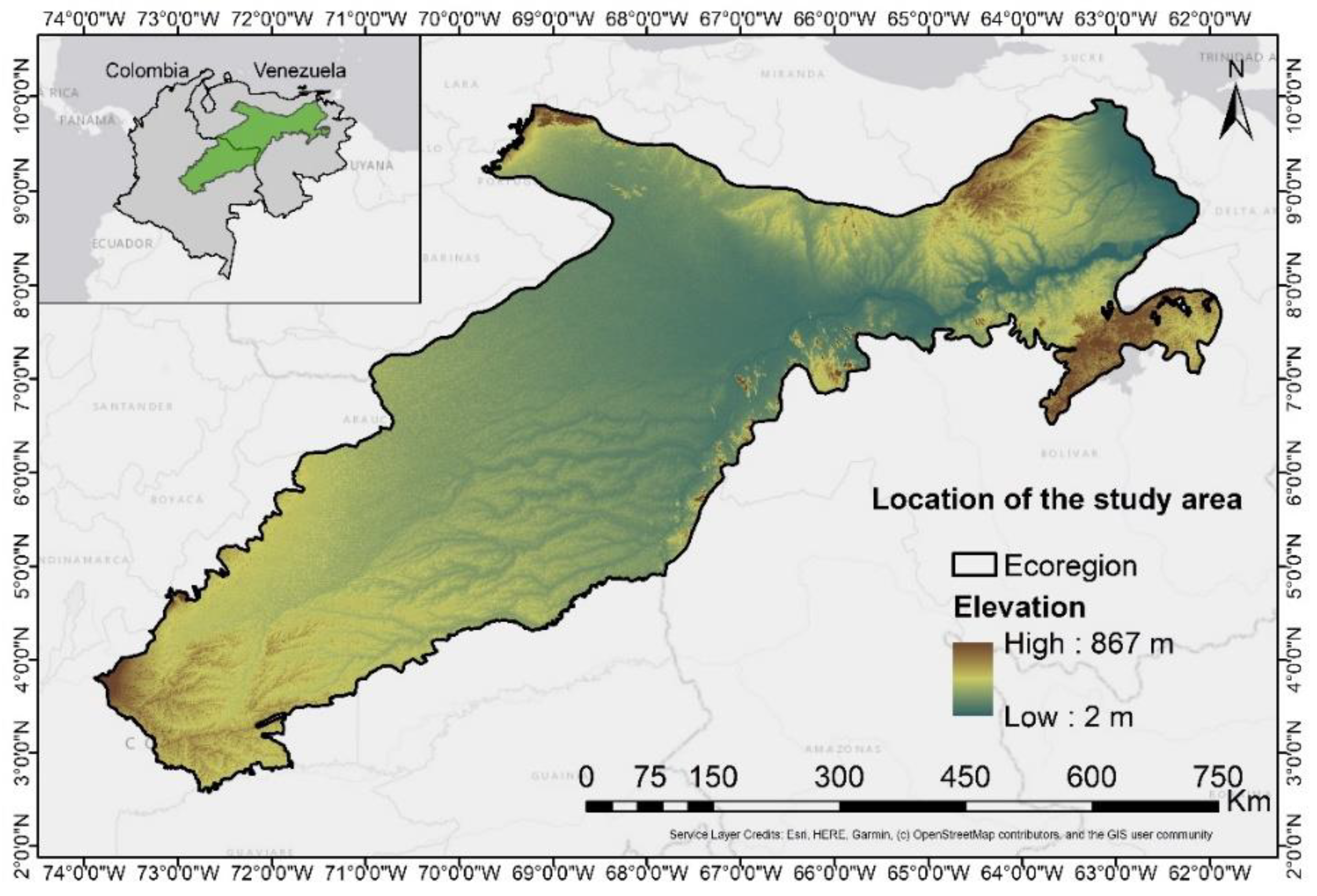
2.1. Study Area

The study area (Figure 1) corresponds to a portion of the plains or llanos ecoregion. This area belongs to a biome of tropical and subtropical grasslands, savannas and shrubs [22], specifically the area that includes the Colombian and Venezuelan plains (73–61° W, 10–2° N), and has an approximate total area of 383.141 km2. The llanos ecoregion is mainly characterized by three ecological determinants: the seasonality of the climate, the low fertility soils, and the frequent presence of burned areas [23].

2.2. Data Collection and Pre-Processing

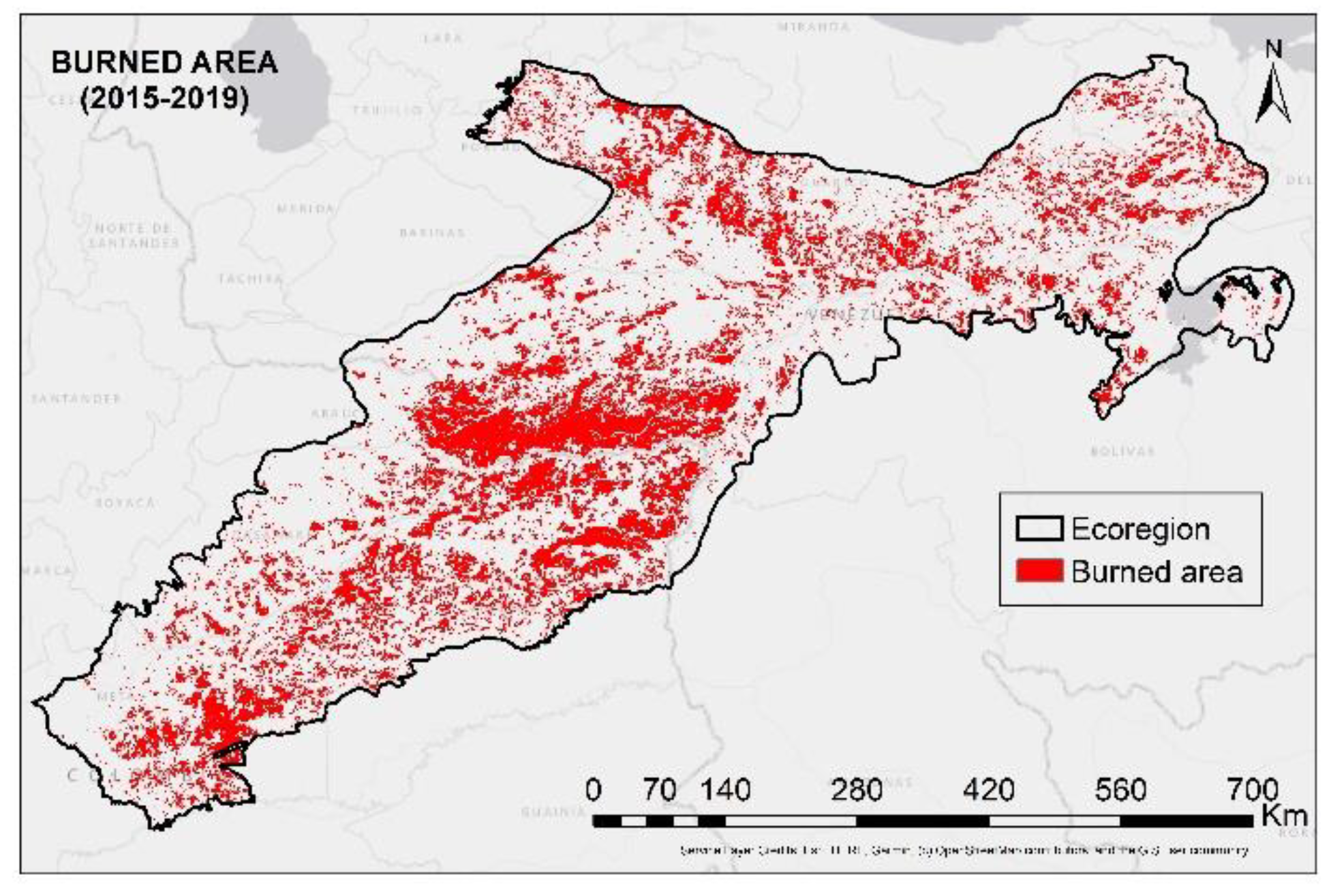
2.2.1. Fire Database

The first stage of the modeling process involved compiling an inventory of fires in the region, because the prediction of future occurrences is based on the assumption that future fires in the same location can be predicted by analyzing data from past occurrences [24]. For historical information on fires in the study area (Figure 2), data was collected on burned areas during the dry season (which occurs between the months of December and March [23]), using data for a period of 5 years [25]; in this case this included the last five years, that is, from 2015 to 2019 (with the exception of 2020 because this new information was used to evaluate the outcome of the zoning process resulting from the model). The product MCD64A1 (version 6) has monthly information at a global level of burned areas with a spatial resolution of 500 m [26]. The algorithm uses reflectance information from Moderate Resolution Imaging Spectroradiometer (MODIS) images (500 m) in conjunction with data from MODIS active fires (1 km) to generate the burned areas by month.

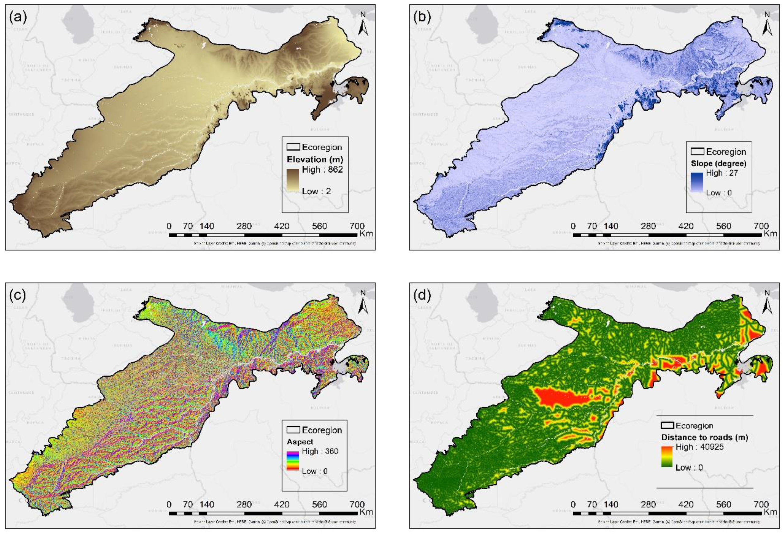
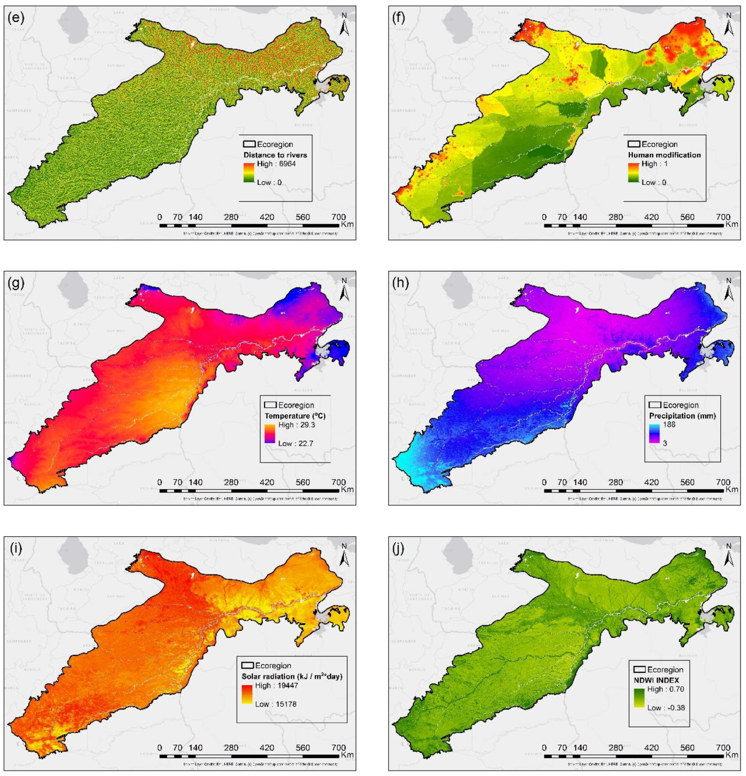
2.2.2. Factors Relating to the Occurrence of Fires

The quantitative evaluation of the probability of the occurrence of fires took into account (in addition to the location of past fires) geo-environmental and anthropogenic predisposing factors [10]. In this work 14 variables were preliminary identified in relation to four types of factors [17]: topographic, presence of human activities, vegetation, and climate, which were all identified and selected based on the availability of information sources. The correct (or incorrect) selection of factors is reflected in the evaluation of the prediction of the resulting models [27].
In relation to topographic variables, the 30 m Shuttle Radar Topography Mission (SRTM) Digital Elevation Model (DEM) was used [28], from which information was extracted for the elevation variable and its derivatives (slope and aspect or direction of the slope). To establish the anthropic presence in the ecoregion, the layers of two entities that allow access and mobility were used: land routes (Global Roads Inventory [29]) and river network (HydroSHEDS: Hydrological Data and Maps Based on Shuttle Elevation Derivatives at Multiple Scales [30]). In addition, we used the CSP gHM Global Human Modification data set that provides a measure of the intensity of human modification on the landscape based on five types of stressors: human settlements, agriculture, transportation, mining/electricity production, and electrical infrastructure [31].
Vegetation indices are used in the field of remote sensing to provide a quantitative and qualitative approximation of the vegetation cover using spectral measurements [32]. Using these indices provides an indication of the state of the vegetation or its moisture content. The information corresponding to the Normalized Difference Vegetation Index (NDVI) and Enhanced Vegetation Index (EVI) indices was derived from the MOD13A1.006 data set that provides the value of the vegetation indices at the pixel level (500 m), which is calculated from information on surface reflectance, after masking water, clouds, cloud shadows, and heavy aerosols [33]. The Normalized Difference Water Index (NDWI) and Visual Atmospheric Resistance Index (VARI) indices were obtained from Landsat 8 image processing. The corresponding equations of the four above-mentioned indices are included in Table 1.
For information on climate variables, we used the WorldClim dataset (version 2.0), which contains monthly climate data for the 1970–2000 period, with high spatial resolution (approximately 1 km2) [39]. The information used from this data set was average temperature (°C) precipitation (mm), solar radiation (kJ m2/day), and wind speed (m s−1) for the months comprising the dry season (December, January, February, and March).

2.2.3. Preprocessing

Google Earth Engine (GEE) is a cloud-based platform that facilitates access to high-performance computing resources to process large volumes of geospatial information without being limited to the characteristics of a local machine [40]. GEE processing services were accessed via R Studio Environment using the R package rgee [41] to collect and pre-process information for factors relating to the probability of occurrence. Some base information layers were downloaded from external sources (weather and roads), but these were also incorporated into the GEE platform to unify the location and availability of the information layers.
For the specific calculation of the slope and aspect variables, the elevation layer and the respective GEE methods were used as base information. In the case of land access roads and rivers, distance rasters were constructed.
For the NDVI and EVI, the average value of these indexes was calculated for the months of December, January, February, and March of the years 2015 to 2019, from the product MOD13A1.006. For the calculation of the NDWI and VARI indices, compositions of Landsat 8 images were constructed (product LANDSAT/LC08/C01/T1_SR) using a cloud masking algorithm for all available images for the study area (1048 images) and averaging the values to derive a single image that represented the average reflectance values of the dry season (December to March) for the years 2015 to 2019. Then, the corresponding equations were applied to calculate the indices, selecting the appropriate bands according to the Landsat 8 satellite.
For the climatic variables (four images for each variable, corresponding to the months of December, January, February, and March) a single image was constructed for each variable, which represented the average value for the dry season.
All information layers were resampled at 500 m in the projected world Mercator coordinate system (EPSG:3395) and cut by the limit of the study area. Additionally, a pair of masks (water surfaces and urban centers) were applied to the information layers so that the pixels corresponding to these two categories did not represent information (no data). The water surface information was obtained from the Joint Research Centre (JRC) Yearly Water Classification History data set, version 1, which provides information on the location and distribution of water bodies globally [42]. In the case of urban centers, the 2018 cover layer of data set MCD12Q1.006 was reclassified, which refers to land cover resulting from the supervised classification of MODIS [43]. The initial list of variables is presented in Table 2. At this point, all geographic information layers, which are GEE-type objects, were converted to R-type objects for further modeling using the R language (R version 3.5.3).

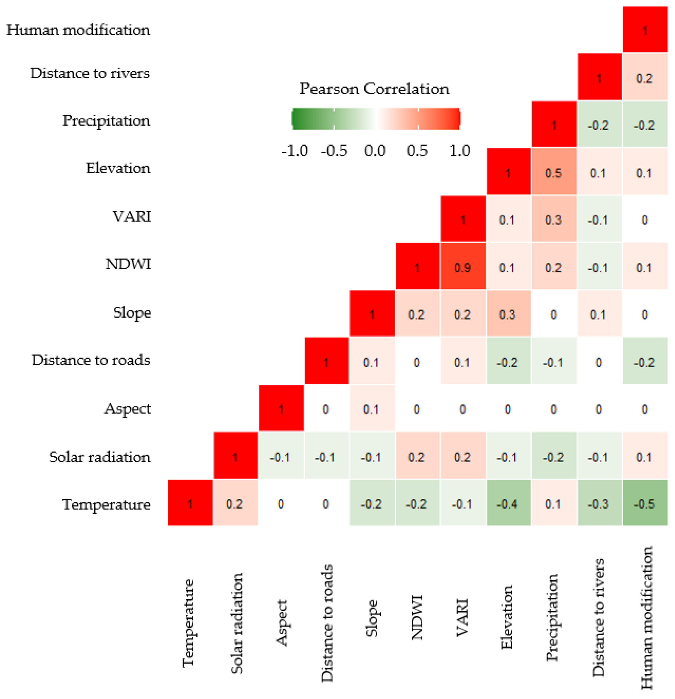
2.3. Variable Selection
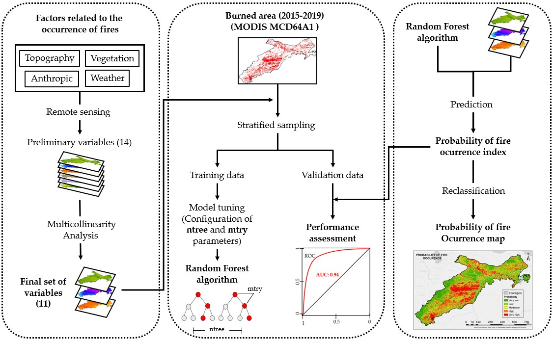
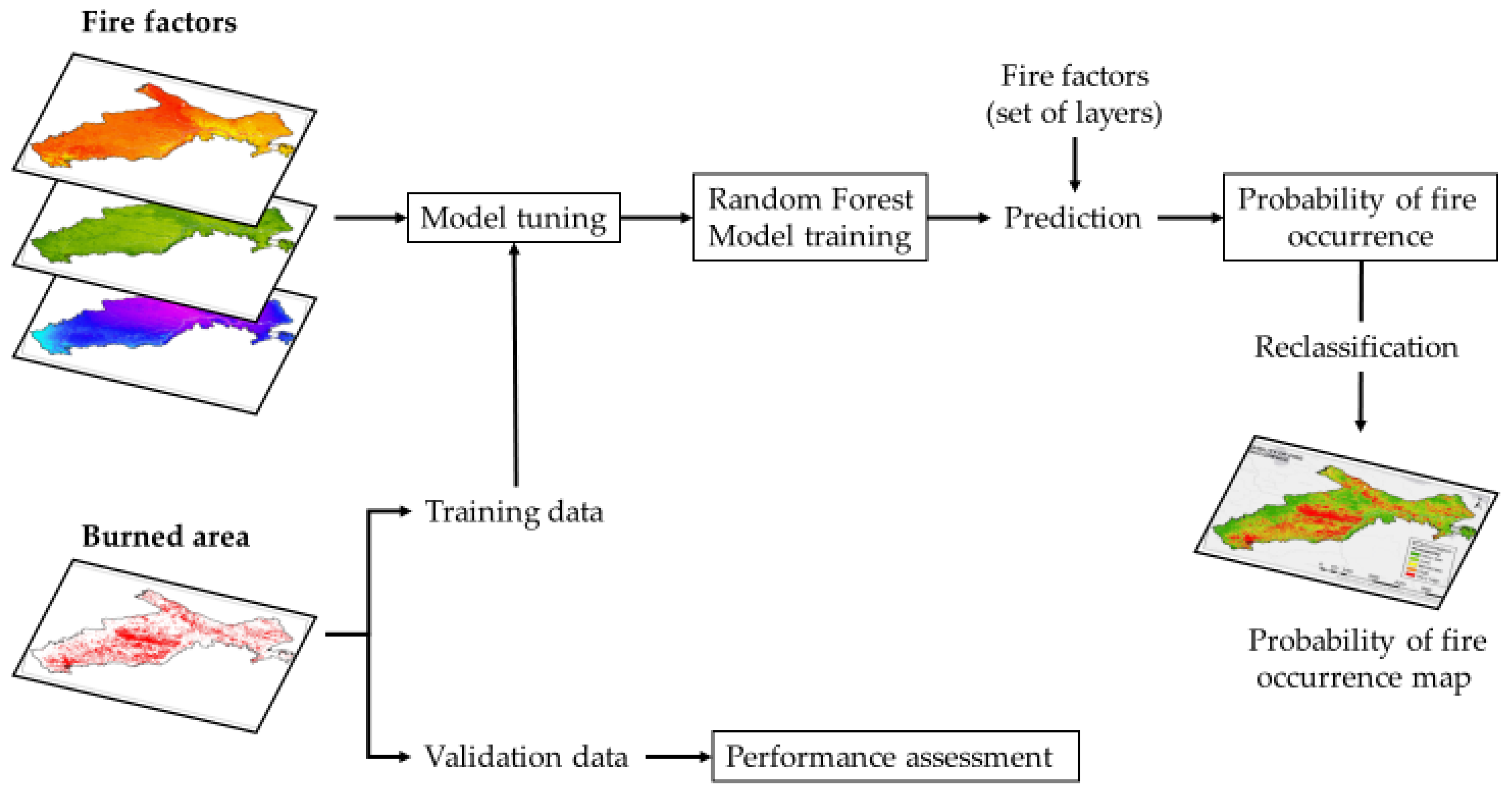
When applying machine learning algorithms it is necessary to make a careful selection of variables because, not only the results in the prediction process from classification models are improved, but also the computation costs for the calculations are reduced and the interpretation of the input data is facilitated [44].
Multicollinearity occurs when two or more predictor variables are highly correlated. This can result in a less accurate estimate due to the effect of an independent variable on the dependent variable, compared to when the independent variables have no correlation between them [45]. To estimate multicollinearity among fire explanatory variables, the variance inflation factor (VIF) was used, which evaluates how much the variance of an estimated value of the regression coefficient increases when predictors are correlated [46]. Specifically, within the environment of R, this analysis contrasts a predictor variable against all others; if one of the variables presents a strong correlation with at least one of the other variables, its correlation coefficient will be close to one and the VIF value for this variable will be large [47]. In general, it is considered that a VIF value greater than 10 represents a significant correlation between the variables [48]. Therefore, those variables with VIF greater than 10 were excluded from the subsequent modeling process, that is, the wind variable and the NDVI and EVI indices (Table 3).
In addition to the VIF, Pearson’s correlation analysis was applied to identify linear correlation relationships between pairs of variables (in the new filtered set of variables). The correlation coefficient of Pearson allows measurement of the association between variables. When a correlation is present, the change in the magnitude of a variable is associated with a change in the magnitude in another variable, either in the same direction (positive coefficient) or in the opposite direction (negative coefficient). This coefficient is scaled and takes values between −1 and 1, where 0 is equivalent to the case in which no correlation exists [49]. A correlation coefficient greater than or equal to 0.7 is considered a correlation indicator that can lead to distortion of the modeling process and affect future predictions [45]. The results suggested an important positive correlation between NDWI and VARI (Figure 3), thus, it was decided to use only the first of these because it is an index widely used in the monitoring of fires and has been proven to have a strong correlation with their occurrence [50].
Figure 4 shows the spatial distribution of the final set of variables used in the process of spatial modeling of the probability of the occurrence of fires in the study area.

3. Methodology

3.1. Random Forest Algorithm
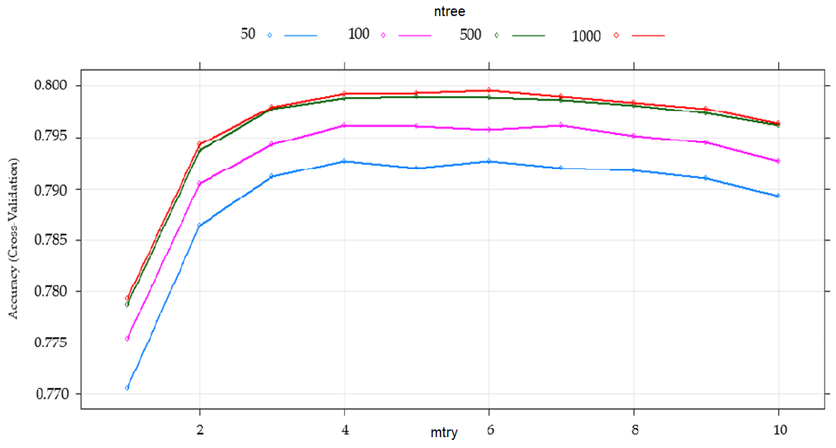
The random forest is an algorithm that averages the predictive values of a large number of classification trees or individual regressions that are determined from a portion (usually 2/3) of the data used for training the model; the remaining sample is used for estimating how well the model performs [51]. From the information layer of burned areas for 2015–2019, a stratified sampling was conducted, in which, for each class (burned area/non-burned area), the same number of points were taken (randomly), for a total of 500,000 points. Of these points, 70% (350,000) were used for model training and the configuration of important model parameters (ntree: number of trees and mtry: number of variables randomly sampled as candidates for each division). The main idea of the algorithm is to combine many decision trees using a series of startup data and choose explanatory variables (Table 3, Figure 5) in each node of the tree [52]. In the context of machine learning, mapping the probability of occurrence of a fire can be interpreted as a binary classification problem in which each pixel can be classified into two classes: fire or no fire [53]. The fire class corresponds to the value of 1, while the non-fire class is 0. The total number of predictions for each class (result of the prediction made by each of the decision trees that make up the random forest algorithm), normalized over the total number of predictions, allows probabilistic results to be obtained [10], which are interpreted as the probability. In the probability of fire occurrence map, the value of each pixel represents the probability that a fire will occur in the future.

3.2. Tuning Model

The most important parameters to be specified in R for the random forest algorithm are the number of decision trees (ntree) and the number of variables randomly sampled as candidates for each division (mtry) [10]. The cross-validation method (CV) consists of subdividing the data set (in this case, the training set) into 10 samples, of which 9 were used to train the model and 1 to validate it; this process was repeated 10 times. The CV method was applied using different value options of the mtry and ntree parameters using the R caret package to select the combination of values that presents the best precision, estimated by the accuracy metric, which refers to the percentage of data correctly classified [54]. The combinations of parameters were tested with respect to four levels of ntree (50, 100, 500, and 1000) and ten levels of mtry (from 1 to 10). The maximum value of ntree tested was 1000, following the recommendation of previous research to maintain stable results [51,55]. The optimal value of the parameters was mtry = 6 and ntree = 1000 (Figure 5).

3.3. Performance Assessment

Validation is the most important component of the modeling process to ensure the results of the models have scientific relevance [56]. Of the original stratified sampling for model construction, we used the remaining 30% (150,000 points) for model validation. To calculate the importance of the variables, we used the Mean Decrease in Accuracy (MDA) [51], which is one of the metrics most used in random forest models [57]. This metric quantifies the importance of a variable by measuring the change in the prediction accuracy when the values of a certain variable are randomly changed from their original observations. Therefore, the change in precision determines the importance of a variable [55]. This measure allows ranking the variables hierarchically according to their importance within the model. The MDA metric was calculated using the importance function available in the random forest package in R [58].
The results of the fire occurrence probability model based on the random forest were verified using the value of the area under the Receiver Operating Characteristics (ROC) curve (AUC) [59]. A ROC curve plots the changes in true prediction rates against false positive prediction rates; the best possible prediction corresponds to a value AUC of the ROC curve of 1, which represents 100% sensitivity (no false negatives) and 100% specificity (no false positives) [56]. Table 4 shows the interpretation of the AUC metric values in relation to the model performance. The term sensitivity refers to the proportion of pixels that represent burned areas and are correctly classified as burned areas; conversely, specificity reflects the pixels that do not correspond to a burned area and are correctly classified as such [53].
Additionally, to test the reliability of the fire probability occurrence map produced by the implementation of the random forest algorithm, the burned area ratio was derived for the classified map and new burned area data (2020). For this purpose, the burned area information layer for the 2020 dry season was overlaid with the result of the occurrence probability zoning process to calculate the burned area presented for each of the probability zones [62].

3.4. Probability of Fire Occurrence

Finally, a prediction was made on the set of raster layers (the predictor variables associated with the occurrence of fire, Figure 4) using the trained random forest model. The new data was evaluated against all decision trees built in the random forest model, in which each tree was assigned a label (fire or no fire), and the label with the most votes was finally selected [63]. The result (in terms of probability) was an index with continuous values between 0–1 that represents the probability of fire occurrence. There are different categorization schemes (e.g., quantile, natural breaks) and each gives rise to different results [64]. In the case of natural breaks, this method is used repeatedly to classify probability indices [25], establishing grouping limits by searching for patterns that are inherent in the data [65]. The result of the probability of occurrence was reclassified into five classes using the natural breaks method.
A general workflow of the applied methodology is summarized in Figure 6.

4. Results

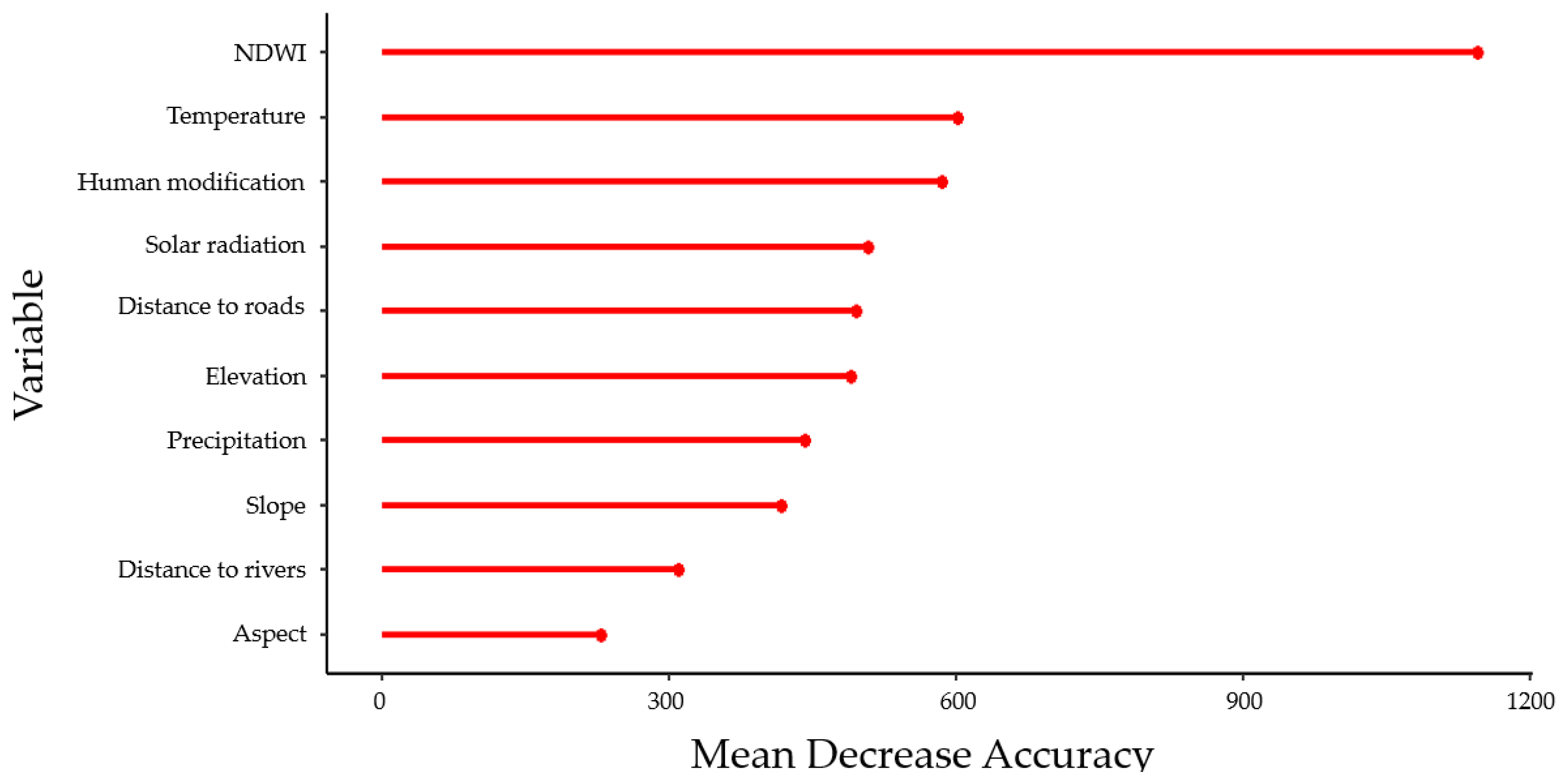
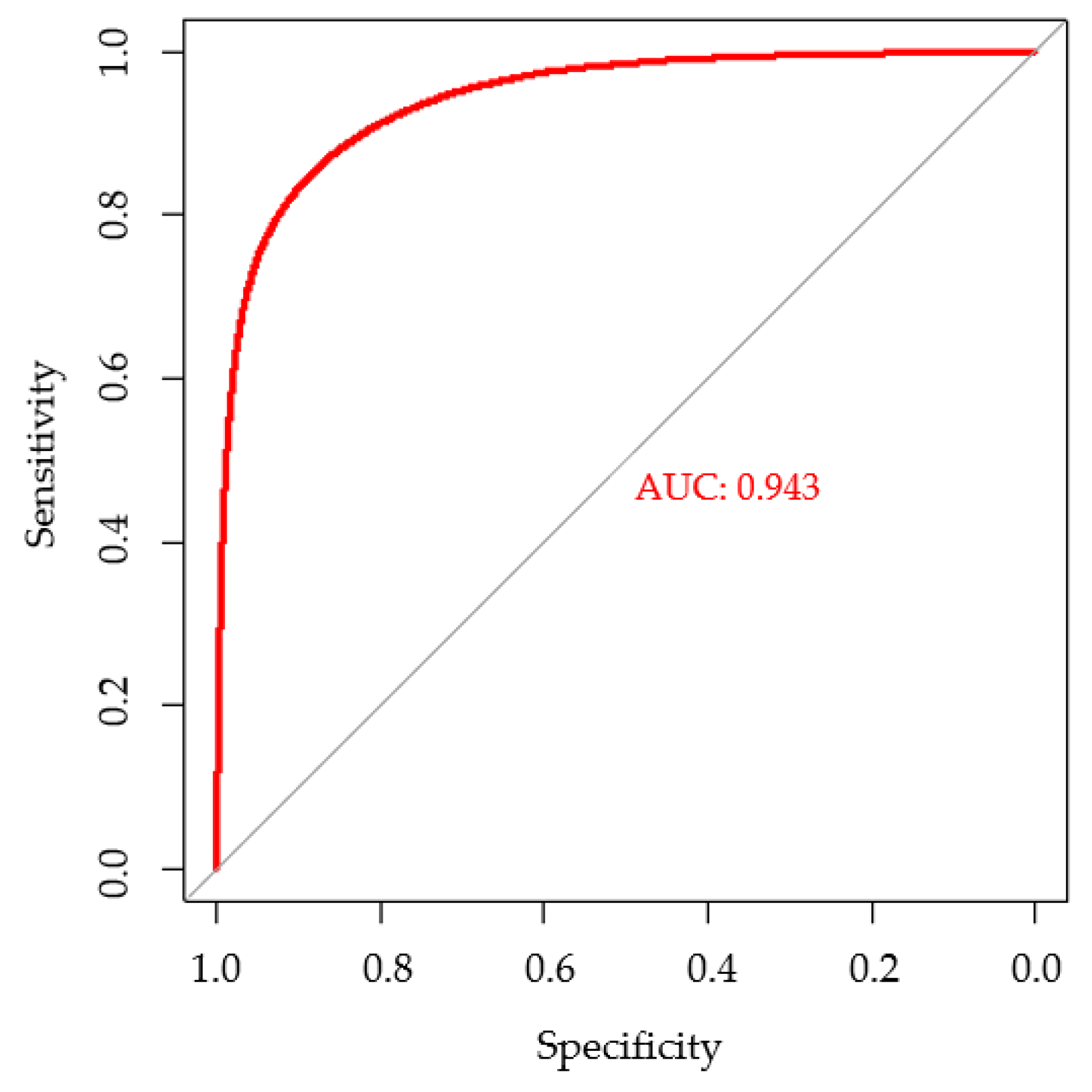
4.1. Predictive Performance and Variable Importance

According to the results presented in Figure 7, the most important variable within the model is the NDWI index (selecting this variable shows the most important change in the accuracy of the model), followed by temperature in second place of importance, and anthropogenic modification in third place. The order of importance follows a group with very similar values in which the variables of precipitation, distance to roads, solar radiation, slope, and elevation are found. Finally, the variables of less importance in the model are the aspect and the distance to rivers.
The accuracy of the fire occurrence model was evaluated using a ROC curve, a common method in the evaluation of the quality of probabilistic prediction models [25]. The result (Figure 8) shows that the AUC of the ROC curve is 0.943.

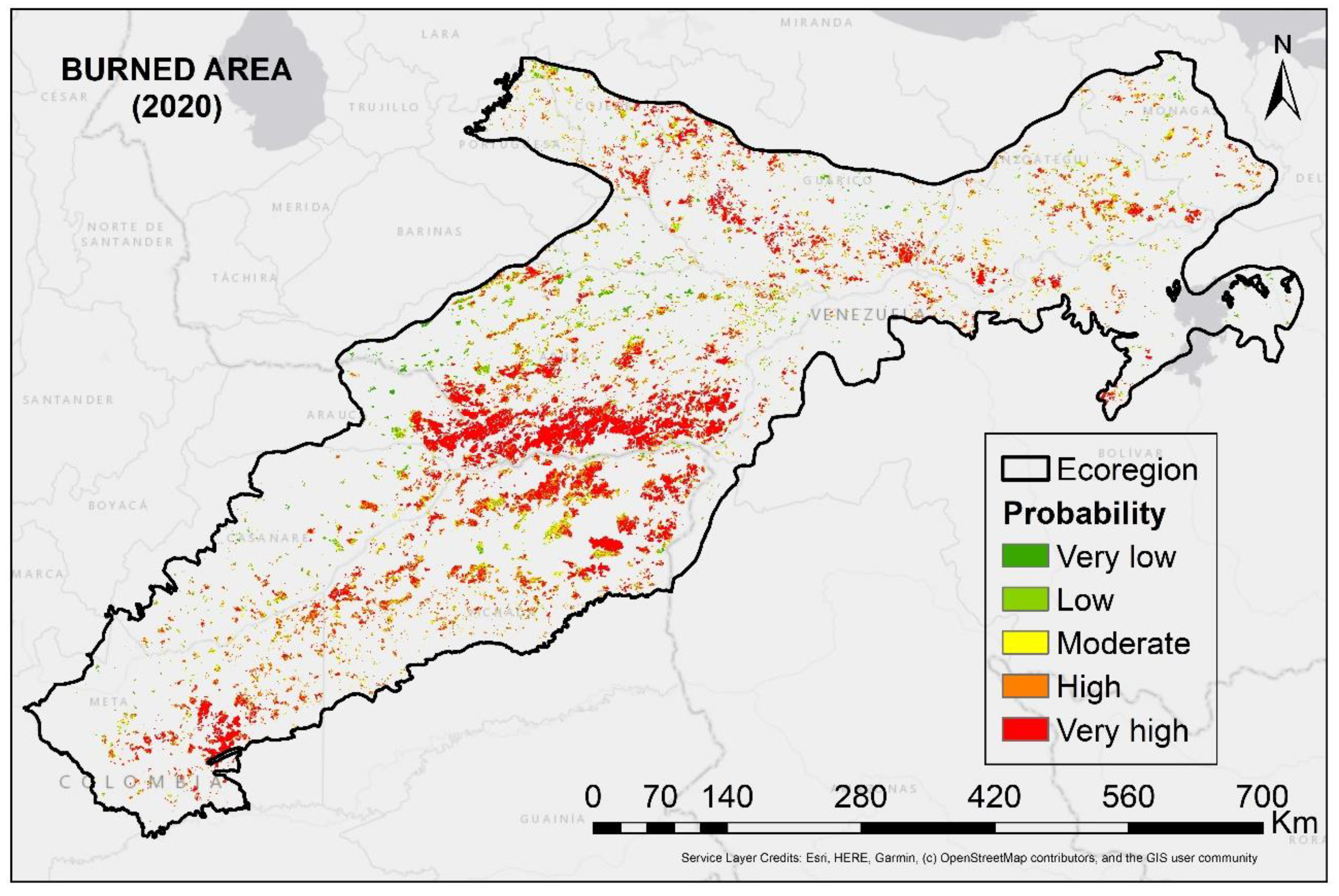
4.2. Probability of Fire Occurrence Map

The result of applying the random forest model to predict the occurrence of fires is a value that expresses the probability of each pixel being burned in the future, under the assumption of a set of predisposing variables [10]. This result was reclassified using the method of natural breaks, resulting in the following classes of probability of occurrence of fires in the study area: very low probability (0–0.16), low probability (0.16–0.36), moderate probability (0.36–0.57), high probability (0.57–0.79), and very high probability (0.79–1), as shown in Figure 9.
Table 5 shows the results of the area corresponding to each zoning level. The very low category covers the largest area (28.2%, 103,982.0 km2), followed by low (23.2%, 85,254.3 km2), very high (17.6%, 64,846.0 km2), moderate (17.2%, 63,267.0 km2), and high (13.8%, 50,879.5 km2).
By overlaying the map of occurrence probability with the burned area of the 2020 dry season, we found that approximately 73% of this occurs in the categories of high and very high occurrence probability, validating the high reliability presented by the model (Figure 10).

5. Discussion

In a recent review document [3] about the applications of machine learning in forest fire science and management, 298 publications were identified (between the years 1996 and 2019), with an important increase during the past 5 years. Among the references, in 71 cases machine learning algorithms were implemented to identify areas susceptible to the occurrence of fire events. The paper highlights that this type of algorithm has been highly successful due to its ability to learn from data and model hidden relationships which, in turn, often present better results than classical statistical approaches [10]. This research presents the first model of probability of fire occurrence specific to the ecoregion of the Colombian-Venezuelan plains. According to the accuracy assessment results undertaken using the metric of the AUC of the ROC curve (value of 0.94), the random forest model shows excellent performance [60,61]. Some works have demonstrated the high predictive capacity of random forests to model the occurrence of fires, presenting higher performance than other types of machine learning algorithms, such as boosted regression trees (BRT), support vector machines (SVM) [66], and maximum entropy (ME) [52].
It is important to take into consideration the seasonality of the fire regime. In this particular case, we focus on one of the two “macro-stations” that the area of study presents [10], specifically during the dry season, which occurs between the months of December and March [23].
The result of the model validation allows us to infer that the choice of variables and their combination worked well to predict the occurrence of fires in the study area during the dry season. The correct choice of variables is the first (and fundamental) step for a successful modeling process [67]. Furthermore, the quality of the model was confirmed by validating the result of the zoning of probability of occurrence with burned area data for 2020, for which around 73% of the new burned area was shown in areas whose category of probability of occurrence is high and very high, indicating a high reliability of the model to predict new occurrences.
Regarding the factors inside the model that influence the occurrence of fire, the most important variable was the NDWI. This index is used to estimate the vegetation cover [37]. It is sensitive to changes in moisture content [68]. Different indices work best according to the type of vegetation, but the moisture content of the fuel is best represented by this particular index [69]. Previous research has shown that NDWI provides better results for estimating the variation in moisture content of living fuel (type herbaceous) and predicting the risk of fire and behavior assessment in the case of savannah ecosystems [70].
The second most important variable was temperature (mean). This might be the result of the direct relationship between fuel humidity and temperature [71]. Increased temperature can lead to increased evaporation from plant cover, which in turn causes a decrease in moisture content, increasing the likelihood of fires by facilitating ignition [72]. Other research has shown the importance of the average temperature, particularly during the dry season (which is when more fires usually occur) and its greater influence on fire occurrence than other climatic variables, such as rainfall or humidity [71]. Indeed, in the dry seasons the potential for the occurrence of fires can be explained to a great extent by the high temperatures and low humidity [73].
The third variable in order of importance was human modification. Although fires may occur due to natural causes, they do not justify the scale or the alarming increase in fires that occurs in vegetation cover. The historical origin of such fires can be defined as the product of a “social aggression that has been taking place towards the forest” [74]. Within the modeling of the probability of occurrence of fires, it is of great importance to consider sources of ignition that are mainly of anthropic origin.

6. Conclusions

The spatial prediction of fire occurrence can be used as a benchmark to better allocate resources in the context of fire management and prevention. This research can support the selection of critical monitoring areas (to better spatially organize resources); organize management practices, such as slash-and-burn (among others) to promote the care and maintenance of the components of the ecosystem; and prevent and minimize the negative effects of fire. We believe that this type of input can be used in decision making, particularly related to questions of where to take action, that is, to answer the question of which locations need special focus [75]. In addition, prioritizing the integral management of fires based on the intrinsic relationship between the humidity of the fuel and high temperatures, the management of vegetable fuel is recommended as a mechanism to control the occurrence of fires, especially in zones of higher temperature. To a significant extent, these two factors determine the dynamics of the occurrence of fires in the ecoregion of the Colombian-Venezuelan plains. Regional scale modeling allows the identification of sites where it would be worthwhile to increase research detail to direct efforts to build specific models at local scales involving spatial information that is not available at smaller scales. For example, weather conditions can be an input variable that allows the construction of models at short temporal scales to predict the imminent presence of fires, which would be beneficial in monitoring and control tasks.
Our research confirms that the combination of data from remote sensing and automatic learning algorithms (specifically the random forest) represents a good tool to model the probability of fire occurrence. Based on this, our research identifies those areas that are more susceptible to these events. The design presented here of the model of fire probability can serve as a guide for other researchers to build models based on basic cartographic data and information from free access global databases, focused on regional analysis and using free tools that allow replicability. Specifically, the processing capacity of Google Earth Engine was used to collect and organize information from different sources. This data was accessed using the R environment, and the method provides an important compatibility between information systems and programming languages, and optimizes the use of information from open access sources.

Author Contributions

Conceptualization, J.S.B. and D.A.; methodology, J.S.B. and D.A.; writing, J.S.B. and D.A.; data collection J.S.B.; data analysis J.S.B. and D.A. All authors have read and agreed to the published version of the manuscript.

Funding

This research was funded by NAS Subaward Letters No 2000007526 (PEER Cycle 5) and No 2000010972 (PEER Cycle 8) funding and the Colombian Administrative Department of Science, Technology and Innovation (Colciencias), project award No 110180863738 (CT-247-2019).

Acknowledgments

We are very grateful to Tania Marisol Gonzalez, Maria Constanza Meza y Laura Isabel Mesa for their continuous support. We would also like to thank Thomas Defler who edited this manuscript for proper English language, grammar, punctuation, spelling, and overall style.

Conflicts of Interest

The authors declare no conflict of interest.

References

  1. Armenteras, D.; Bernal, F.H.; González, F.; Morales, M.; Pabón, J.D.; Páramo, G.E.; González Alonso, F.; Morales, M.; Pabón Caicedo, J.; Páramo Rocha, G.; et al. Incendios de la Cobertura Vegetal en Colombia, Primera ed.; Parra, Á., Ed.; Universidad Autónoma de Occidente: Cali, Colombia, 2011; ISBN 9789588713021. [Google Scholar]
  2. Martell, D. Forest fire management, current practices and new challenges for operational researchers. In Handbook of Operations Research in Natural Resources, International Series in Operations Research & Management Science; Weintraub, A., Romero, C., Bjorndal, T., Epstein, R., Eds.; Springer: New York, NY, USA, 2007; Volume 99, pp. 419–506. ISBN 9788476661987. [Google Scholar]
  3. Jain, P.; Coogan, S.C.P.; Subramanian, S.G.; Crowley, M.; Taylor, S.; Flannigan, M.D. A review of machine learning applications in wildfire science and management. arXiv 2020, arXiv:2003.00646. [Google Scholar] [CrossRef]
  4. Giglio, L.; Boschetti, L.; Roy, D.P.; Humber, M.L.; Justice, C.O. The Collection 6 MODIS burned area mapping algorithm and product. Remote Sens. Environ. 2018, 217, 72–85. [Google Scholar] [CrossRef]
  5. Ngoc Thach, N.; Bao-Toan Ngo, D.; Xuan-Canh, P.; Hong-Thi, N.; Hang Thi, B.; Nhat-Duc, H.; Tien Bui, D. Spatial pattern assessment of tropical forest fire danger at Thuan Chau area (Vietnam) using GIS-based advanced machine learning algorithms: A comparative study. Ecol. Inform. 2018, 46, 74–85. [Google Scholar] [CrossRef]
  6. Tien Bui, D.; Hung Le, V.; Hoang, N.-D.; Dieu, T.B.; Hung, V. GIS-Based Spatial Prediction of Tropical Forest Fire Danger Using a New Hybrid Machine Learning Method. Ecol. Inform. 2018, 48, 104–116. [Google Scholar] [CrossRef]
  7. North, B.M.P.; Stephens, S.L.; Collins, B.M.; Agee, J.; Aplet, G.; Franklin, J.F.; Fulé, P.Z. Reform forest fire management. Science 2015, 349, 1280–1281. [Google Scholar] [CrossRef] [PubMed]
  8. Bachmann, A.; Allgöwer, B. A consistent wildland fire risk terminology is needed! Fire Manag. Today 2001, 61, 28–33. [Google Scholar]
  9. Hurley, M.J.; Gottuk, D.; Hall, J.R.; Harada, K.; Kuligowski, E.; Puchovsky, M.; Torero, J.; Watts, J.M.; Wieczorek, C. Introduction to Fire Risk Analysis. In SFPE Handbook of Fire Protection Engineering; Springer: New York, NY, USA, 2016; pp. 1–3493. ISBN 9781493925650. [Google Scholar]
  10. Tonini, M.; D’Andrea, M.; Biondi, G.; Degli Esposti, S.; Trucchia, A.; Fiorucci, P. A Machine Learning-Based Approach for Wildfire Susceptibility Mapping. The Case Study of the Liguria Region in Italy. Geosciences 2020, 10, 105. [Google Scholar] [CrossRef] [Green Version]
  11. Nami, M.H.; Jaafari, A.; Fallah, M.; Nabiuni, S. Spatial prediction of wildfire probability in the Hyrcanian ecoregion using evidential belief function model and GIS. Int. J. Environ. Sci. Technol. 2018, 15, 373–384. [Google Scholar] [CrossRef]
  12. Tien Bui, D.; Bui, Q.T.; Nguyen, Q.P.; Pradhan, B.; Nampak, H.; Trinh, P.T. A hybrid artificial intelligence approach using GIS-based neural-fuzzy inference system and particle swarm optimization for forest fire susceptibility modeling at a tropical area. Agric. For. Meteorol. 2017, 233, 32–44. [Google Scholar] [CrossRef]
  13. Calviño-Cancela, M.; Chas-Amil, M.L.; García-Martínez, E.D.; Touza, J. Interacting effects of topography, vegetation, human activities and wildland-urban interfaces on wildfire ignition risk. For. Ecol. Manag. 2017, 397, 10–17. [Google Scholar] [CrossRef] [Green Version]
  14. Jaiswal, R.K.; Mukherjee, S.; Raju, K.D.; Saxena, R. Forest fire risk zone mapping from satellite imagery and GIS. Int. J. Appl. Earth Obs. Geoinf. 2002, 4, 1–10. [Google Scholar] [CrossRef]
  15. FAO Fire management—Global assessment 2006. FAO For. Pap. 2007, 151, 135.
  16. Adab, H.; Kanniah, K.D.; Solaimani, K.; Sallehuddin, R. Modelling static fire hazard in a semi-arid region using frequency analysis. Int. J. Wildl. Fire 2015, 24, 763–777. [Google Scholar] [CrossRef]
  17. Sayad, Y.; Mousannif, H.; Al Moatassime, H. Predictive modeling of wildfires: A new dataset and machine learning approach. Fire Saf. J. 2019, 104, 130–146. [Google Scholar] [CrossRef]
  18. Rodrigues, M.; De La Riva, J.; Fotheringham, S. Modeling the spatial variation of the explanatory factors of human-caused wildfires in Spain using geographically weighted logistic regression. Appl. Geogr. 2014, 48, 52–63. [Google Scholar] [CrossRef]
  19. Soares-Filho, B.; Silvestrini, R.; Nepstad, D.; Brando, P.; Rodrigues, H.; Alencar, A.; Coe, M.; Locks, C.; Lima, L.; Hissa, L.; et al. Forest fragmentation, climate change and understory fire regimes on the Amazonian landscapes of the Xingu headwaters. Landsc. Ecol. 2012, 27, 585–598. [Google Scholar] [CrossRef]
  20. Armenteras, D.; Rodríguez, N.; Retana, J. Landscape Dynamics in Northwestern Amazonia: An Assessment of Pastures, Fire and Illicit Crops as Drivers of Tropical Deforestation. PLoS ONE 2013, 8, e54310. [Google Scholar] [CrossRef] [Green Version]
  21. Silvestrini, R.A.; Soares-Filho, B.S.; Nepstad, D.; Coe, M.; Rodrigues, H.; Assuncao, R. Simulating fire regimes in the Amazon in response to climate change and deforestation. Ecol. Appl. 2011, 21, 1573–1590. [Google Scholar] [CrossRef]
  22. Dinerstein, E.; Olson, D.; Joshi, A.; Vynne, C.; Burgess, N.; Wikramanayake, E.; Hahn, N.; Palminteri, S.; Hedao, P.; Noss, R.; et al. An Ecoregion-Based Approach to Protecting Half the Terrestrial Realm. Bioscience 2017, 67, 534–545. [Google Scholar] [CrossRef]
  23. Chacón, E.; Ulloa, A.; Llambí, L.; Acevedo, D.; Utrera, A. Paisajes Y Ecosistemas Llaneros: Ecología Y Conservación. In Tierras Llaneras de Venezuela …tierras de Buena Esperanza; Lopez, R., Hétier, J., López, D., Schargel, R., Zinck, A., Eds.; Consejo de Publicaciones de la Universidad de Los Andes: Mérida, Venezuela, 2015; pp. 195–240. ISBN 9789801117810. [Google Scholar]
  24. Tehrany, M.S.; Jones, S. Evaluating the variations in the flood susceptibility maps accuracies due to the alterations in the type and extent of the flood inventory. Int. Arch. Photogramm. Remote Sens. Spat. Inf. Sci. -ISPRS Arch. 2013, 42, 209–214. [Google Scholar] [CrossRef] [Green Version]
  25. Ghorbanzadeh, O.; Blaschke, T.; Gholamnia, K.; Aryal, J. Forest Fire Susceptibility and Risk Mapping Using Social/Infrastructural Vulnerability and Environmental Variables. Fire 2019, 2, 50. [Google Scholar] [CrossRef] [Green Version]
  26. Giglio, L.; Justice, C.; Boschetti, L.; Roy, D. MCD64A1 MODIS/Terra+Aqua Burned Area Monthly L3 Global 500m SIN Grid V006 [Data set]. NASA EOSDIS Land Process. DAAC 2015. [CrossRef]
  27. Verde, J.; Zêzere, J. Assessment and validation of wildfire susceptibility and hazard in Portugal. Nat. Hazards Earth Syst. Sci. 2010, 10, 485–497. [Google Scholar] [CrossRef]
  28. Farr, T.; Rosen, P.; Caro, E.; Crippen, R.; Duren, R.; Hensley, S.; Kobrick, M.; Palller, M.; Rodriguez, E.; Roth, L.; et al. The Shuttle Radar Topography Mission. Rev. Geophys. 2007, 45, 1–33. [Google Scholar] [CrossRef] [Green Version]
  29. Meijer, J.R.; Huijbregts, M.A.J.; Schotten, K.C.G.J.; Schipper, A.M. Global patterns of current and future road infrastructure. Environ. Res. Lett. 2018, 13, 064006. [Google Scholar] [CrossRef] [Green Version]
  30. Grill, G.; Lehner, B.; Thieme, M.; Geenen, B.; Tickner, D.; Antonelli, F.; Babu, S.; Borrelli, P.; Cheng, L.; Crochetiere, H.; et al. Mapping the world’s free-flowing rivers. Nature 2019, 569, 215–221. [Google Scholar] [CrossRef]
  31. Kennedy, C.M.; Oakleaf, J.R.; Theobald, D.M.; Baruch-Mordo, S.; Kiesecker, J. Managing the middle: A shift in conservation priorities based on the global human modification gradient. Glob. Chang. Biol. 2019, 25, 811–826. [Google Scholar] [CrossRef]
  32. Bannari, A.; Morin, D.; Bonn, F.; Huete, A.R. A review of vegetation indices. Remote Sens. Rev. 1995, 13, 95–120. [Google Scholar] [CrossRef]
  33. Didan, K. MOD13A1 MODIS/Terra Vegetation Indices 16-Day L3 Global 500m SIN Grid V006 [Data set]. NASA EOSDIS Land Process. DAAC 2015. [Google Scholar] [CrossRef]
  34. Running, S. Estimating Terrestrial Primary Productivity by Combining Remote Sensing and Ecosystem Simulation. In Remote Sensing of Biosphere Functioning; Hobbs, R.J., Mooney, H.A., Eds.; Springer: New York, NY, USA, 1990; pp. 65–86. ISBN 978-1-4612-3302-2. [Google Scholar]
  35. Huete, A.; Didan, K.; Miura, T.; Rodrigeuz, E.; Gao, X.; Ferreira, L. Overview of the radiometric and biophysical performance of the MODIS vegetation indices. Remote Sens. Environ. 2002, 83, 213. [Google Scholar] [CrossRef]
  36. Gao, B.-C. NDWI—A Normalized Difference Water Index for Remote Sensing of Vegetation Liquid Water from Space. Remote Sens. Environ. 1996, 58, 257–266. [Google Scholar] [CrossRef]
  37. Huang, J.; Chen, D.; Cosh, M.H. Sub-pixel reflectance unmixing in estimating vegetation water content and dry biomass of corn and soybeans cropland using normalized difference water index (NDWI) from satellites. Int. J. Remote Sens. 2009, 30, 2075–2104. [Google Scholar] [CrossRef]
  38. Gitelson, A.A.; Kaufman, Y.J.; Stark, R.; Rundquist, D. Novel algorithms for remote estimation of vegetation fraction. Remote Sens. Environ. 2002, 80, 76–87. [Google Scholar] [CrossRef] [Green Version]
  39. Fick, S.E.; Hijmans, R.J. WorldClim 2: New 1-km spatial resolution climate surfaces for global land areas. Int. J. Climatol. 2017, 37, 4302–4315. [Google Scholar] [CrossRef]
  40. Gorelick, N.; Hancher, M.; Dixon, M.; Ilyushchenko, S.; Thau, D.; Moore, R. Google Earth Engine: Planetary-scale geospatial analysis for everyone. Remote Sens. Environ. 2017, 202, 18–27. [Google Scholar] [CrossRef]
  41. Aybar, C.; Wu, Q.; Bautista, L.; Yali, R.; Barja, A. An R package for interacting with Google Earth Engine. J. Open Source Softw. 2020, 2020, 2272. [Google Scholar] [CrossRef]
  42. Pekel, J.F.; Cottam, A.; Gorelick, N.; Belward, A.S. High-resolution mapping of global surface water and its long-term changes. Nature 2016, 540, 418–422. [Google Scholar] [CrossRef]
  43. Sulla-Menashe, D.; Friedl, M.A. User Guide to Collection 6 MODIS Land Cover (MCD12Q1 and MCD12C1) Product; USGS: Reston, VA, USA, 2018; pp. 1–18. [CrossRef]
  44. Martínez-Álvarez, F.; Reyes, J.; Morales-Esteban, A.; Rubio-Escudero, C. Determining the best set of seismicity indicators to predict earthquakes. Two case studies: Chile and the Iberian Peninsula. Knowl. -Based Syst. 2013, 50, 198–210. [Google Scholar] [CrossRef]
  45. Dormann, C.F.; Elith, J.; Bacher, S.; Buchmann, C.; Carl, G.; Carré, G.; Marquéz, J.R.G.; Gruber, B.; Lafourcade, B.; Leitão, P.J.; et al. Collinearity: A review of methods to deal with it and a simulation study evaluating their performance. Ecography 2013, 36, 027–046. [Google Scholar] [CrossRef]
  46. Akinwande, M.O.; Dikko, H.G.; Samson, A. Variance Inflation Factor: As a Condition for the Inclusion of Suppressor Variable(s) in Regression Analysis. Open J. Stat. 2015, 05, 754–767. [Google Scholar] [CrossRef] [Green Version]
  47. Naimi, B.; Hamm, N.A.S.; Groen, T.A.; Skidmore, A.K.; Toxopeus, A.G. Where is positional uncertainty a problem for species distribution modelling? Ecography 2014, 37, 191–203. [Google Scholar] [CrossRef]
  48. Wu, W.; Zhang, L. Comparison of spatial and non-spatial logistic regression models for modeling the occurrence of cloud cover in north-eastern Puerto Rico. Appl. Geogr. 2013, 37, 52–62. [Google Scholar] [CrossRef]
  49. Schober, P.; Schwarte, L.A. Correlation coefficients: Appropriate use and interpretation. Anesth. Analg. 2018, 126, 1763–1768. [Google Scholar] [CrossRef] [PubMed]
  50. Chowdhury, E.H.; Hassan, Q.K. Operational perspective of remote sensing-based forest fire danger forecasting systems. ISPRS J. Photogramm. Remote Sens. 2015, 104, 224–236. [Google Scholar] [CrossRef]
  51. Breiman, L. Random Forests. Mach. Learn. 2001, 45, 32. [Google Scholar] [CrossRef] [Green Version]
  52. Arpaci, A.; Malowerschnig, B.; Sass, O.; Vacik, H. Using multi variate data mining techniques for estimating fire susceptibility of Tyrolean forests. Appl. Geogr. 2014, 53, 258–270. [Google Scholar] [CrossRef]
  53. Tien Bui, D.; Le, K.T.T.; Nguyen, V.C.; Le, H.D.; Revhaug, I. Tropical forest fire susceptibility mapping at the Cat Ba National Park area, Hai Phong City, Vietnam, using GIS-based Kernel logistic regression. Remote Sens. 2016, 8, 347. [Google Scholar] [CrossRef] [Green Version]
  54. Kuhn, M. Building Predictive Models in R Using the caret Package. J. Stat. Softw. 2008, 28, 1–26. [Google Scholar] [CrossRef] [Green Version]
  55. Guo, F.; Wang, G.; Su, Z.; Liang, H.; Wang, W.; Lin, F.; Liu, A. What drives forest fire in Fujian, China? Evidence from logistic regression and Random Forests. Int. J. Wildl. Fire 2016, 25, 505–519. [Google Scholar] [CrossRef]
  56. Jaafari, A.; Gholami, D.M.; Zenner, E.K. A Bayesian modeling of wildfire probability in the Zagros Mountains, Iran. Ecol. Inform. 2017, 39, 32–44. [Google Scholar] [CrossRef]
  57. Schmidt, A.; Niemeyer, J.; Rottensteiner, F.; Soergel, U. Contextual classification of full waveform lidar data in the wadden sea. IEEE Geosci. Remote Sens. Lett. 2014, 11, 1614–1618. [Google Scholar] [CrossRef]
  58. Genuer, R.; Poggi, J.M.; Tuleau-Malot, C. Variable selection using random forests. Pattern Recognit. Lett. 2010, 31, 2225–2236. [Google Scholar] [CrossRef] [Green Version]
  59. Hanley, J.; McNeil, B. The Meaning and Use of the Area under a Receiver Operating Characteristic (ROC) curve. Radiology 1982, 143, 29–36. [Google Scholar] [CrossRef] [PubMed] [Green Version]
  60. Mccune, B.; Grace, J. Analysis of Ecological Communities; MJM Software Design: Gleneden Beach, OR, USA, 2002. [Google Scholar]
  61. Hosmer, D.; Lemeshow, S.; Sturdivant, R. Applied Logistic Regression, 3rd ed.; John Wiley & Sons: Hoboken, NJ, USA, 2013. [Google Scholar]
  62. Pourghasemi, H.R.; Pradhan, B.; Gokceoglu, C. Application of fuzzy logic and analytical hierarchy process (AHP) to landslide susceptibility mapping at Haraz watershed, Iran. Nat. Hazards 2012, 63, 965–996. [Google Scholar] [CrossRef]
  63. Belgiu, M.; Drăgu, L. Random forest in remote sensing: A review of applications and future directions. ISPRS J. Photogramm. Remote Sens. 2016, 114, 24–31. [Google Scholar] [CrossRef]
  64. Tehrany, M.S.; Pradhan, B.; Jebur, M.N. Flood susceptibility mapping using a novel ensemble weights-of-evidence and support vector machine models in GIS. J. Hydrol. 2014, 512, 332–343. [Google Scholar] [CrossRef]
  65. Xiao, J.; Shen, Y.; Ge, J.; Tateishi, R.; Tang, C.; Liang, Y.; Huang, Z. Evaluating urban expansion and land use change in Shijiazhuang, China, by using GIS and remote sensing. Landsc. Urban Plan. 2006, 75, 69–80. [Google Scholar] [CrossRef]
  66. Rodrigues, M.; De la Riva, J. An insight into machine-learning algorithms to model human-caused wildfire occurrence. Environ. Model. Softw. 2014, 57, 192–201. [Google Scholar] [CrossRef]
  67. Eskandari, S. A new approach for forest fire risk modeling using fuzzy AHP and GIS in Hyrcanian forests of Iran. Arab. J. Geosci. Roma 2017, 10, 190. [Google Scholar] [CrossRef]
  68. Peterson, S.H.; Roberts, D.A.; Dennison, P.E. Mapping live fuel moisture with MODIS data: A multiple regression approach. Remote Sens. Environ. 2008, 112, 4272–4284. [Google Scholar] [CrossRef]
  69. Maki, M.; Ishiahra, M.; Tamura, M. Estimation of leaf water status to monitor the risk of forest fires by using remotely sensed data. Remote Sens. Environ. 2004, 90, 441–450. [Google Scholar] [CrossRef]
  70. Verbesselt, J.; Somers, B.; Lhermitte, S.; Jonckheere, I.; van Aardt, J.; Coppin, P. Monitoring herbaceous fuel moisture content with SPOT VEGETATION time-series for fire risk prediction in savanna ecosystems. Remote Sens. Environ. 2007, 108, 357–368. [Google Scholar] [CrossRef]
  71. Guo, F.; Su, Z.; Wang, G.; Sun, L.; Tigabu, M.; Yang, X.; Hu, H. Understanding fire drivers and relative impacts in different Chinese forest ecosystems. Sci. Total Environ. 2017, 605, 411–425. [Google Scholar] [CrossRef] [PubMed]
  72. Bisquert, M.; Caselles, E.; Snchez, J.M.; Caselles, V. Application of artificial neural networks and logistic regression to the prediction of forest fire danger in Galicia using MODIS data. Int. J. Wildl. Fire 2012, 21, 1025–1029. [Google Scholar] [CrossRef]
  73. Huesca, M.; Litago, J.; Palacios-Orueta, A.; Montes, F.; Sebastián-López, A.; Escribano, P. Assessment of forest fire seasonality using MODIS fire potential: A time series approach. Agric. For. Meteorol. 2009, 149, 1946–1955. [Google Scholar] [CrossRef]
  74. CFS Aspects sociaux, economiques et culturels des incendies de forêts en Italie. In Proceedings of the Seminar on Forest Fire Prevention, Land Use and People; ECE/FAO/OIT: Athens, Greece, 1987.
  75. Taubenböck, H.; Post, J.; Roth, A.; Zosseder, K.; Strunz, G.; Dech, S. A conceptual vulnerability and risk framework as outline to identify capabilities of remote sensing. Nat. Hazards Earth Syst. Sci. 2008, 8, 409–420. [Google Scholar] [CrossRef]
Figure 1. Location map of the study area.
Remotesensing 12 03921 g001
Figure 2. Spatial distribution of burned areas during the dry season (December to March), during the period 2015–2019.
Remotesensing 12 03921 g002
Figure 3. Pearson correlation.
Remotesensing 12 03921 g003
Figure 4. Forest fire variables: (a) elevation; (b) slope; (c) aspect; (d) distance to roads; (e) distance to rivers; (f) human modification; (g) temperature; (h) precipitation; (i) solar radiation; (j) Normalized Difference Water Index (NDWI).
Remotesensing 12 03921 g004aRemotesensing 12 03921 g004b
Figure 5. Results of the cross-validation process with different configurations of the mtry and ntree values.
Remotesensing 12 03921 g005
Figure 6. General diagram of the methodology used.
Remotesensing 12 03921 g006
Figure 7. Mean Decrease Accuracy value for the variables used in the model.
Remotesensing 12 03921 g007
Figure 8. Receiver Operating Characteristics (ROC) curve and AUC of the random forest model using the validation dataset.
Remotesensing 12 03921 g008
Figure 9. Fire probability map for the study area.
Remotesensing 12 03921 g009
Figure 10. Categorization of the probability of occurrence of fires in relation to the area burned in the year 2020.
Remotesensing 12 03921 g010
Table 1. General equations of the spectral indices used in this study. Bands: NIR: Near Infrared, MIR: Mid-Infrared.
IndexGeneral Equation
NDVI [34] NIR     RED NIR   +   RED
EVI [35] 2.5 × ( NIR     RED NIR   +   6   ×   RED     7.5   ×   BLUE   +   1 )
NDWI [36,37] MIR     NIR MIR   +   NIR
VARI [38] GREEN     RED GREEN   +   RED     BLUE
Table 2. Variables, units, and sources of information.
VariableUnitsSource
ElevationMetersDEM SRTM
AspectDegreesDEM SRTM
SlopeDegreesDEM SRTM
Distance to roadsMetesGlobal Roads Inventory Project
Distance to riversMetersHydroSHEDS
Anthropic modificationIntensityCSP gHM
NDVIIndexMOD13A1.006
EVIIndexMOD13A1.006
NDWIIndexLandsat 8 images
VARIIndexLandsat 8 images
PrecipitationmmWorldClim V2
Solar radiationkJ m2/dayWorldClim V2
Temperature°CWorldClim V2
Winds velocitym/sWorldClim V2
Table 3. Variance inflation factor (VIF) values.
VariableVIF
Aspect1.03
Distance to roads1.14
Distance to rivers1.18
Slope1.40
Human modification1.73
Solar radiation2.44
Elevation3.49
Temperature5.75
Precipitation6.26
NDWI8.44
VARI8.88
Winds11.95
EVI13.93
NDVI14.68
Table 4. Interpretation of area under the curve (AUC) values in relation to model performance [60,61].
AUC ValuesModel Performance
0.5–0.6Poor
0.6–0.7Moderate
0.7–0.8Good
0.8–0.9Very good
>0.9Excellent
Table 5. Fire probability by categories.
Fire Probability (%)CategoryArea (km2)% Area
0–16Very low103,982.028.2
16–16Low85,254.323.2
16–57Moderate63,267.017.2
57–79High50,879.513.8
79–100Very high64,846.017.6
Publisher’s Note: MDPI stays neutral with regard to jurisdictional claims in published maps and institutional affiliations.

