Next Article in Journal
Robust Loop Closure Detection Integrating Visual–Spatial–Semantic Information via Topological Graphs and CNN Features
Next Article in Special Issue
Fusion of Rain Radar Images and Wind Forecasts in a Deep Learning Model Applied to Rain Nowcasting
Previous Article in Journal
Using Wavelet Transforms to Fuse Nighttime Light Data and POI Big Data to Extract Urban Built-Up Areas
Previous Article in Special Issue
An Effective High Spatiotemporal Resolution NDVI Fusion Model Based on Histogram Clustering
 
 
Correction published on 14 June 2022, see Remote Sens. 2022, 14(12), 2841.
Article

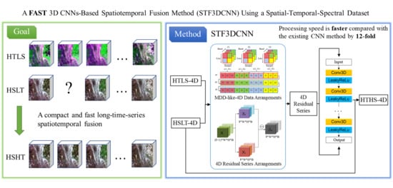
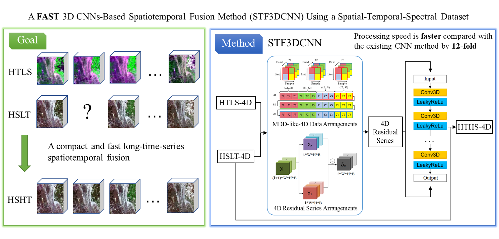
A Fast Three-Dimensional Convolutional Neural Network-Based Spatiotemporal Fusion Method (STF3DCNN) Using a Spatial-Temporal-Spectral Dataset

1
The State Key Laboratory of Remote Sensing Science, Aerospace Information Research Institute, Chinese Academy of Sciences, Beijing 100101, China
2
University of Chinese Academy of Sciences, Beijing 100049, China
*
Author to whom correspondence should be addressed.
Remote Sens. 2020, 12(23), 3888; https://doi.org/10.3390/rs12233888
Submission received: 1 November 2020 / Revised: 25 November 2020 / Accepted: 26 November 2020 / Published: 27 November 2020 / Corrected: 14 June 2022

Abstract

:
With the growing development of remote sensors, huge volumes of remote sensing data are being utilized in related applications, bringing new challenges to the efficiency and capability of processing huge datasets. Spatiotemporal remote sensing data fusion can restore high spatial and high temporal resolution remote sensing data from multiple remote sensing datasets. However, the current methods require long computing times and are of low efficiency, especially the newly proposed deep learning-based methods. Here, we propose a fast three-dimensional convolutional neural network-based spatiotemporal fusion method (STF3DCNN) using a spatial-temporal-spectral dataset. This method is able to fuse low-spatial high-temporal resolution data (HTLS) and high-spatial low-temporal resolution data (HSLT) in a four-dimensional spatial-temporal-spectral dataset with increasing efficiency, while simultaneously ensuring accuracy. The method was tested using three datasets, and discussions of the network parameters were conducted. In addition, this method was compared with commonly used spatiotemporal fusion methods to verify our conclusion.

Graphical Abstract

1. Introduction

With the rapid development of remote sensing applications and sensors, huge amounts of data have accumulated, making long-term monitoring-related applications possible. Various satellites have acquired massive datasets with different spatial and temporal resolutions. Due to the limitations of satellite sensors, remote sensing datasets cannot have both high spatial and high temporal resolutions. Combining the advantages of different remote sensing products to obtain datasets with both high spatial and high temporal resolutions has been a growing research division. Spatiotemporal data fusion is an effective choice to accomplish this goal. However, due to the design of the algorithms, traditional methods and deep learning methods cannot fuse long time-series datasets with a high speed, making them difficult to apply to large, long time-series datasets. They are insufficient because the number of remote sensing datasets continues to grow, and the application requirements have also brought challenges to the processing of long time-series datasets.
To date, researchers have proposed many spatiotemporal fusion methods, which can be divided into three categories [1]: weight function methods, linear optimization decomposition methods, and nonlinear optimization methods (as shown in Table 1). The weight function method assumes a linear relationship between high-spatial low-temporal (HSLT) resolution images and low-spatial high-temporal (HTLS) resolution images and factors temporal, spatial, and spectral weights into the model. The pixel center of the sliding window is used to determine the center pixel value. This method originated from the spatial and temporal adaptive reflectance fusion model (STARFM) [2], and scholars have since made improvements, such as the spatial temporal adaptive algorithm for mapping reflectance change model (STAARCH) [3], an enhanced STARFM (ESTARFM) algorithm [4], a modified version of the ESTARFM (mESTARFM) [5], and a rigorously weighted spatiotemporal fusion model (RWSTFM) [6]. The advantage of the weight function method is that the model is intuitive and widely used, but it has the following problems: (1) objects with changing shapes and short-term transient changes cannot be well predicted, (2) the correlation between sensors has not been strictly proven, and (3) the size of the sliding window and other parameters must be set manually and cannot be obtained automatically. The linear optimization decomposition method is also based on a linear assumption similar in principle to the weight function method. The restored image is obtained by adding constraints to obtain the optimal solution. Based on the optimization criteria, the linear optimization decomposition method can be divided into three sub-categories: the spectral unmixing method, the Bayesian method, and the sparse representation method. Commonly used algorithms include the multisensor multiresolution technique (MMT) spectral unmixing algorithm [7], flexible spatiotemporal data fusion (FSDAF) [8], the spatial and temporal data fusion model (STDFM) algorithm [9], the enhanced STDFM [10], the modified spatial and temporal data fusion approach [11], soft clustering [12], and the object-based spatial and temporal vegetation index unmixing model algorithm (Object Based Image Analysis, OBIA) [13]. Although the weight-based fusion algorithm using linear optimization decomposition can achieve better spatiotemporal fusion reconstruction, it is difficult to satisfy the actual imaging scenario due to the assumption of the linear model. The nonlinear mapping method is based on the deep learning method, which can describe the nonlinear relationship well. Scholars have also explored the use of deep learning methods for spatiotemporal fusion. Moosavi combined a wavelet algorithm, artificial neural network, adaptive neuro-fuzzy inference system, and supported vector machine methods to propose the prediction-phase wavelet–artificial intelligence fusion approach algorithm for Landsat thermal infrared data [14]. In recent years, the use of convolutional neural networks (CNNs or ConvNets) for spatiotemporal fusion algorithms, such as the spatiotemporal fusion using deep convolutional neural networks (STFDCNN) [15] and the deep convolutional spatiotemporal fusion network (DCSTFN) [16], have also been proposed. The nonlinear optimization method can learn and accurately describe the nonlinear relationship between the known and missing time-phase images and has more mobility and accuracy than those of the linear optimization decomposition method. However, its ability is related to the network architectures and parameters. Poor network structures cannot produce good results, and they often require a large number of training samples and a long training time.
All the traditional datasets arrange remote sensing data into three dimensions, space (height and width) and spectrum, rendering the data difficult to rearrange and process when it comes to long time-series. Zhang et al. proposed the idea of a new multi-dimensional dataset (MDD) in 2017 [17] that can build a spatial-temporal-spectral dataset integrating the information in four dimensions. The MDD can satisfy the multi-feature correlation analysis of different dimensions and thus is a good choice for long time-series dataset fusion. This raises the question of how to extract the spatiotemporal information from four-dimensional (4D) datasets. Recently, three-dimensional convolutional neural networks (3D CNNs) have become widely used in video and computer vision fields. Compared with two-dimensional convolutional neural networks (2D CNNs), in which operations are only performed spatially, 3D CNNs perform convolution and pooling operations spatiotemporally, making them well-suited for spatiotemporal feature learning [18].
Based on the above-mentioned reasons, we propose a fast spatiotemporal remote sensing fusion method using the tools of 3D CNNs. Differently from current spatiotemporal fusion methods, our method arranges datasets based on the idea of the MDD, and the calculations are performed four-dimensionally. The method introduces the concept of residual series of the 4D long time-series dataset, to subtract the images of the former dates from latter dates (for example, the dates are arranged and indexed, and we subtract the images on the even dates from those of the odd dates) and pile them in the temporal order. The architecture learns the mappings between 4D residual series of HTLS and HSLT datasets using the 3D CNNs model. By adding predicted residual series of HSHT to the original HSLT dataset, the method can restore a compact 4D long time-series dataset in high spatial and high temporal (HSHT) resolution. The method is easy to implement and of a high efficiency, and it is able to guarantee the accuracy at the same time. The potential contribution of our method may lie in the following: (1) This is, according to the investigation of the authors, the first spatiotemporal remote sensing data fusion method performed four-dimensionally. This casts new light on remote sensing fusion methods. (2) This method has a fast speed compared to other state-of-the-art spatiotemporal fusion methods. It can cut down the processing time hugely, thus shrinking the overall time of long time-series-related remote sensing projects.
This paper is structured as follows. Section 2 presents the overall idea and framework of the proposed method. Section 3 introduces the datasets used to verify the method, the experimental settings, and the ablation study of the method. Section 4 presents a comparison of the results with those of existing spatiotemporal fusion methods. Section 5 summarizes this work.

2. Materials and Methods

Our method is based on the idea of MDD, and the data are arranged and operated 4-dimensionally. Then, a 4D residual series of the dataset is generated and input into the three-dimensional convolutional neural networks (3D CNNs) model to learn the features and the mappings between HTLS and HSLT. The ideas and methods are explained as follows.

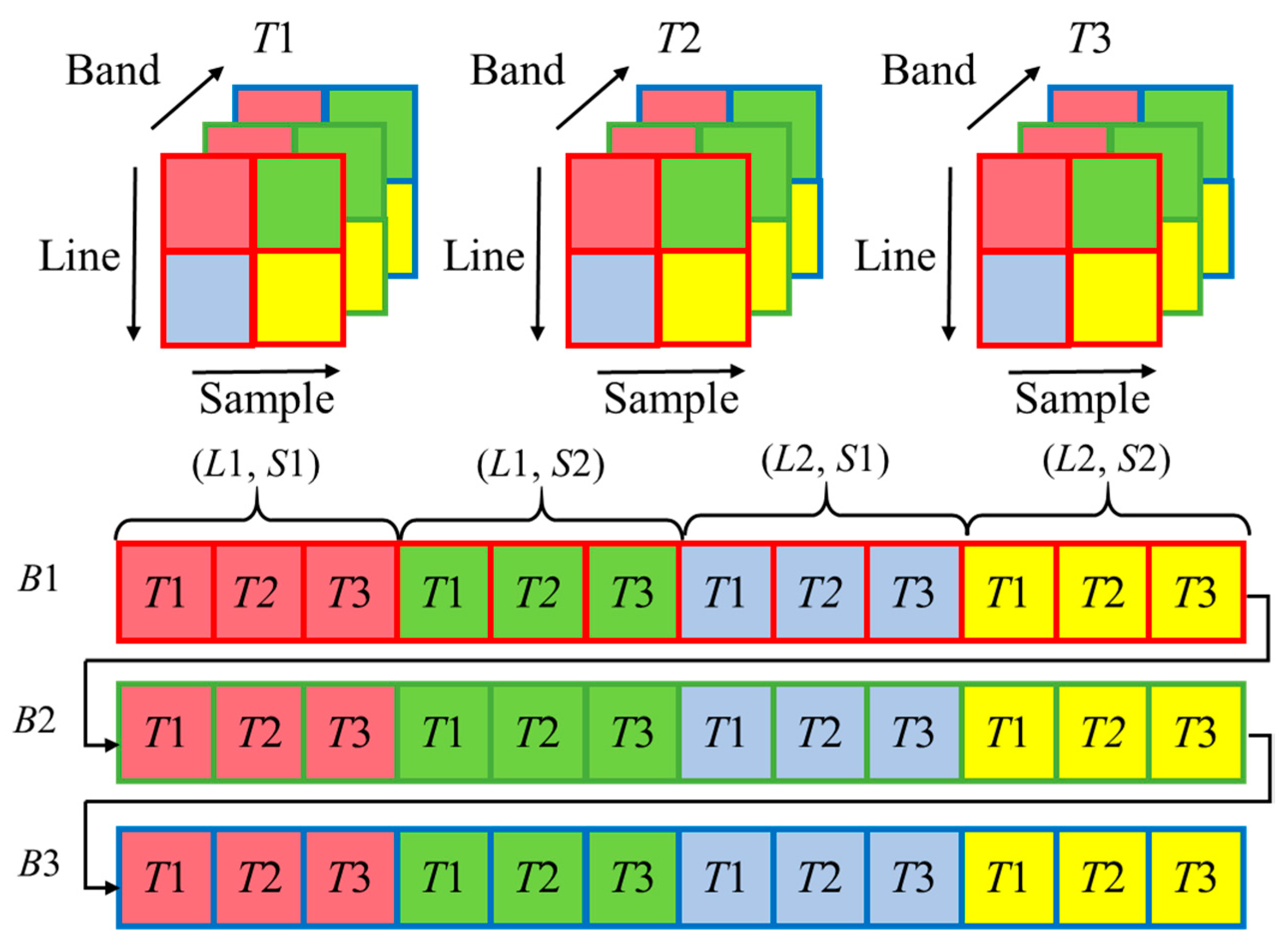
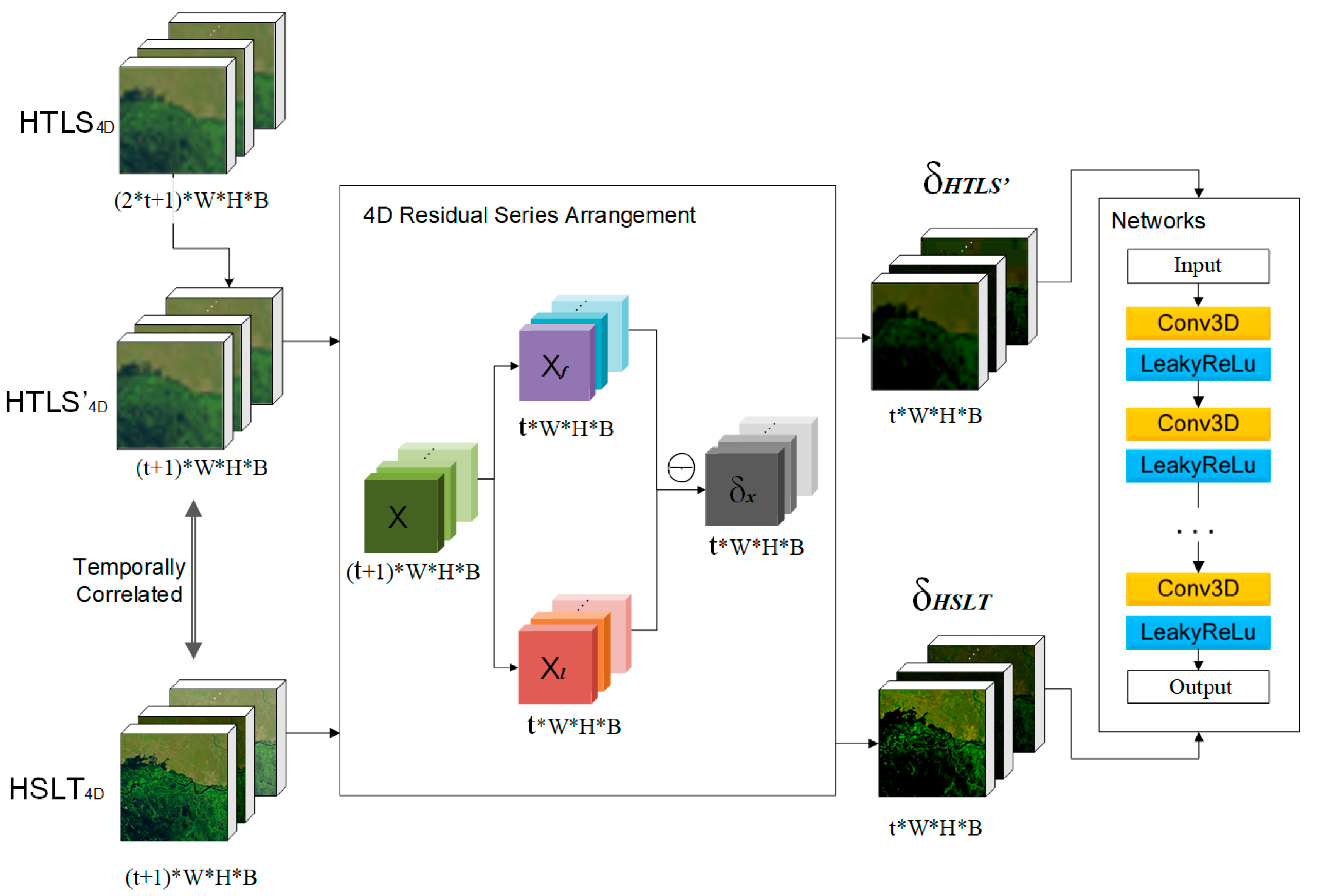
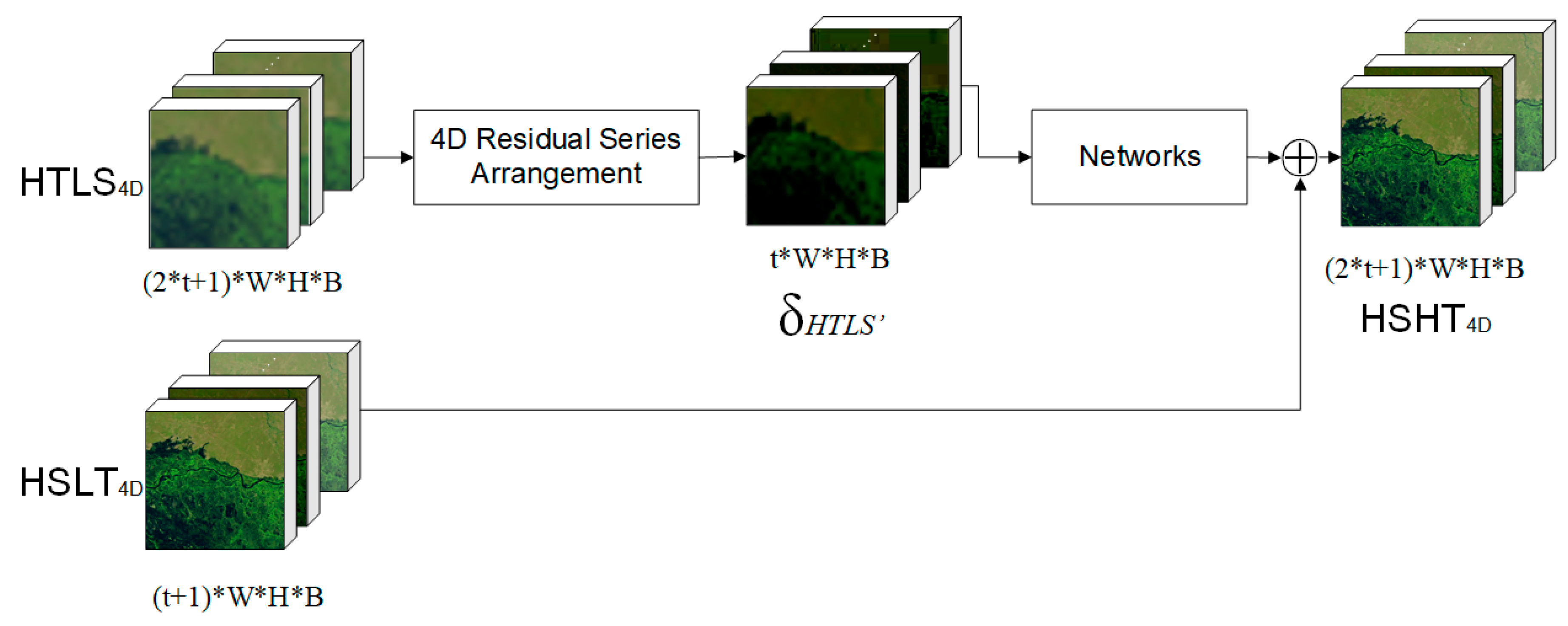
2.1. Four-Dimensional (4D) Residual Series

The existing remote sensing datasets are based mostly on 3D datasets, in which temporal arrangements are not included [19]. The fast 3-dimensional convolutional neural network-based spatiotemporal fusion method (STF3DCNN) draws on the idea of multidimensional datasets in the four-dimensional mode [17]. The MDD arranges data in four dimensions: time, space (height and width), and spectrum. The storage structure of MDD is called SPATS (SPAtial-Temporal-Spectral). It mainly consists of five data formats, and each has different forms of data arrangements. They are: Temporal Sequential in Band (TSB), Temporal Sequential in Pixel (TSP), Temporal Interleaved by Band (TIB), Temporal Interleaved by Pixel (TIP), and Temporal Interleaved by Spectrum (TIS). Similar to the TIP structure shown in Figure 1, our method first organizes data in chronological order. Then, the data are stored in the order of “row first, column second”. Finally, the data are arranged in a spectral order.
In this method, the images in the remote sensing data series are arranged into a 4-dimensional data X R T × W × H × B , where T is the temporal length, W is the image width, H is the image height, and B is the number of bands. Here, we sort the dates sequentially and index them from 1 to T. The data subset X f of former dates t f is generated by Formula (1):
X f = X ( t f , x , y , b ) ,
where t f { 1 , 3 , , T } , x { 1 , 2 , , W } , y { 1 , 2 , , H } , and b { 1 , 2 , , B } . Additionally, the data subset X l of latter dates t l can be represented as:
X l = X ( t l , x , y , b ) ,
where t l { 2 , 4 , , T 1 } . Thus, the residual series of dataset X as δ X can be calculated using Formulas (1) and (2):
δ X = X l X f ,
Here, we present the specific datasets used in the spatiotemporal fusion. We define the 4-dimensional dataset of HTLS as H T L S 4 D R T C × W × H × B and the 4-dimensional dataset of HSLT as H S L T 4 D R T F × W × H × B , where T C = T F × w + 1 and w represents the temporal resolution scale factor. The temporal resolution scale factor is calculated by dividing the temporal resolution of HSLT by that of HTLS. For example, the temporal resolution scale factor of the 8-day Moderate Resolution Imaging Spectroradiometer (MODIS) data and 16-day Landsat data is 2. As their temporal resolutions differ, we generate the temporally correlated subset H T L S 4 D R T F × W × H × B from H T L S 4 D according to the same/nearby dates of the H S L T 4 D . The residual series of H T L S 4 D , H T L S 4 D , and H S L T 4 D are calculated as δ H T L S , δ H T L S , and δ H S L T using Formula (3).

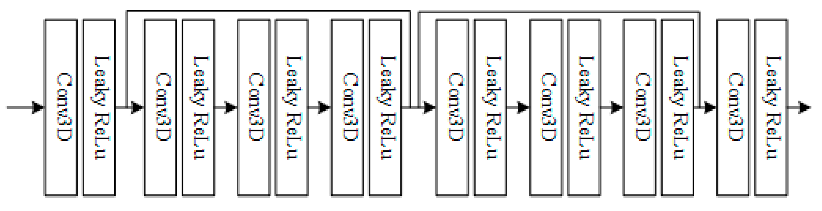
2.2. 3D CNNs for 4D Residual Series

The residual series δ C and δ F are used for training the spatiotemporal 3D CNNs model, the layers of which can be represented as:
h i l ( x , y , z ) = σ ( b i l + k u , v , w h k l 1 ( x u , y v , z w ) W k i l ( u , v , w ) ) ,
where h i l and h k l 1 are the i th 3D feature data in the l th layer and the k th 3D feature data in the previous l 1 th layer, respectively. W k i l is the 3D convolutional filter and the ( u , v , w ) represents a point in the filter. b i l is the 3D bias. σ ( ) is the nonlinear activation function, such as the rectified linear unit function.
Here, the 3D CNNs is used to extract the features across temporal residuals and spatial dimensions. Then, datasets H S L T 4 D and δ H T L S are used to predict the restored HSHT dataset H T H S 4 D R T C × W × H × B . Because some details of the extracted features are aborted when passing pooling layers [20], we choose not to use pooling layers and simply use the simple structure of fully convolutional layers.

2.3. Overall Frame

Here, we use HTLS 4 D , HSLT 4 D , and HTHS 4 D to represent the HTLS, HSLT, and HSHT series with four-dimensional structures. The main idea of this method is to learn the mappings between the residual series of HTLS 4 D and HSLT 4 D . The architecture contains two main parts: the 4D residual series arrangements and the 4D residual feature mapping networks. First, the 4D residual series arrangements arrange the HSLT images and HTLS images into a 4D residual series dataset using Formulas (1)–(3). The 4D residual feature mapping networks are used to learn and extract the features of temporal residuals and spatial dimensions 4-dimensionally. The architecture of the mapping networks is simple and lightweight. It consists of several fully convolutional networks, after which leaky rectified linear unit layers are set to add nonlinearity and reduce the effect of overfitting.
The flow chart of the training stage is shown in Figure 2. In the training stage, the original HTLS4D dataset is first used to generate a subset according to the same/nearest dates of the HSLT4D. That is, it selects images of HTLS with the same/nearest dates to the HSLT and arranges them in the 4D dataset, defined as HTLS’4D. As the inputs for the training process, the HTLS’4D and the HSLT4D are first preprocessed with 4D residual spatial arrangements to obtain the 4D residual series of the HTLS’4D and the HSLT4D dataset, which we represent as δ H T L S and δ H S L T . Then, the 4D residual series are input into the 4D residual mapping networks for training. The δ H T L S is set as the network input and the δ H S L T is set as the network output.
Figure 3 shows the predicting stage of STF3DCNN. Here, the HTLS4D is firstly preprocessed with the 4D residual spatial arrangements to obtain the 4D residual series δ H T L S . Then, the δ H T L S is input into the networks to predict the simulated 4D residual series of the HSHT dataset. Finally, the 4D residual series of the HSHT dataset is added to the HSLT4D, and, together with the original HSLT4D, the predicted HSTH4D is generated.

3. Experiments and Datasets

3.1. Datasets

To validate the effectiveness of the method, the following three datasets were used in the experiment.
(I) The Coleambally Irrigation Area (CIA) dataset is an open-source remote sensing dataset of a rice irrigation system located in southern New South Wales, Australia (34.0034° E, 145.0675° S), and is widely used in time-series remote sensing research [21]. It contains 17 pairs of cloud-free Landsat 7 Enhanced Thematic Mapper and Moderate Resolution Imaging Spectroradiometer (MODIS) data (MOD09GA) sensed during the 2001–2002 summer growing season. All the Landsat data underwent atmospheric correction using MODTRAN4. The CIA dataset overlaps two adjacent paths, and the total area is 2193 km 2 (1720 columns × 2040 lines, 25 m resolution upsampled by the data producer using nearest neighbor). For simplification, all the scenes are cropped to 1500 columns × 2000 lines. This dataset is a good sample for evaluating seasonal changes with complicated landcovers.
(II) The Lower Gwydir Catchment (LGC) dataset is another open-source remote sensing dataset sensed in the northern part of New South Wales (149.2815° E, 29.0855° S) from April 2004 to April 2005 [21]. It consists of 14 pairs of cloudless Landsat 5 Thematic Mapper and MODIS data (MOD09GA) with 3200 columns × 2720 lines at a 25 m spatial resolution. All the Landsat data underwent atmospheric correction using MODTRAN4. MODIS data contain irregular salt-and-pepper noise that is difficult to remove and may cause more distortion. Simulation is often used in spatiotemporal experiments, thus here we used a similar method to that used in Reference [8] which arranges MODIS-like data using Landsat data, and added 40 dBW of Gaussian white noise to simulate approximately the signal-to-noise ratio (SNR) of MODIS data, as shown in Reference [22]. For simplification, all the scenes were cropped to 3000 columns × 2500 lines. On the 10th date of the time-series data, a flood occurred in this field, making this dataset a good sample of a long time-series with abrupt changes, and it is more unpredictable and irregular than the CIA dataset.
(III) The Real Dataset (RDT) was sensed in Williams, CA, USA (122°15′34.33″ W, 39°10′4.17″ N), from June to October 2013. It consists of nine pairs of Landsat 8 Operational Land Imager and MODIS data (MOD09A1) with the spatial resolution of 30 m. Each scene was cropped to 800 columns × 800 lines. A subset of four bands was used. All the data were preprocessed using geographic registration and atmospheric correction. The MODIS data were resampled to the same resolution as that of the Landsat data using the bilinear resampling algorithm. This dataset is a good sample for evaluating seasonal changes in crop fields and vegetated mountain areas.
To download the Landsat–MODIS imagery of CIA and LGC datasets, see http://dx.doi.org/10.4225/08/5111AC0BF1229 for the CIA dataset and http://dx.doi.org/10.4225/08/5111AD2B7FEE6 for the LGC dataset. The acquisition dates and band information used in the experiments are listed in Table 2 and Table 3.

3.2. Data Preprocessing and Experimental Settings

In order to assess our method, we reduced the actual acquisition rate of the Landsat images to two intervals. We used all the MODIS data series and Landsat data on the odd dates to predict the missing scenes on the even dates, and the reference images were the Landsat images on the even dates. The MODIS data in the CIA and LGC datasets were upsampled to 25 m using nearest neighbor interpolation, which is the preprocess conducted by the data producer and has a negative effect on our method. Thus, we retrieved the original 500 m MODIS data using the same method. Then, all the MODIS data in the three datasets were upsampled to the same spatial resolution using the bilinear resampling algorithm according to the need of our method.
The experiments were conducted using Python with Keras 2.0. The graphics processing unit used for acceleration was the NVIDIA Quadro P6000, and the central processing unit used was the Intel Xeon Silver 4110. For the STF3DCNN, the Adam optimization algorithm was used: the learning rate was set to 0.001 and the batch size was 32. The loss function was mean least square. For better optimization, reducing on the plateau and early stopping strategies were used. The learning rate was reduced by a factor of 0.2 when the loss did not change within 5 epochs, and the training was stopped if the loss did not change within 15 epochs. The original number of epochs for training was set to 1000. To test the accuracy and efficiency of the different experiments, fusion quality indices and running time were utilized. The indices used were:
(1)
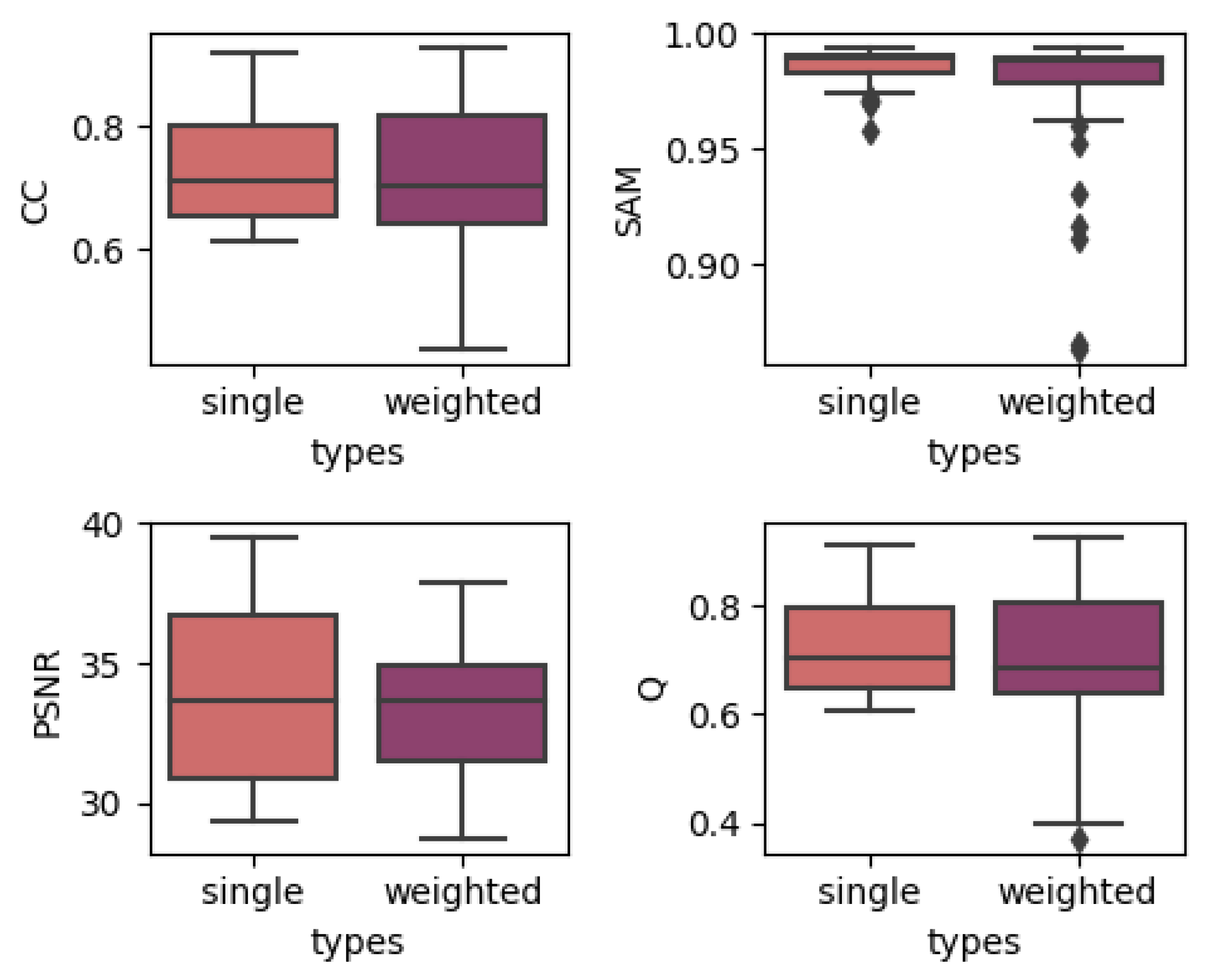
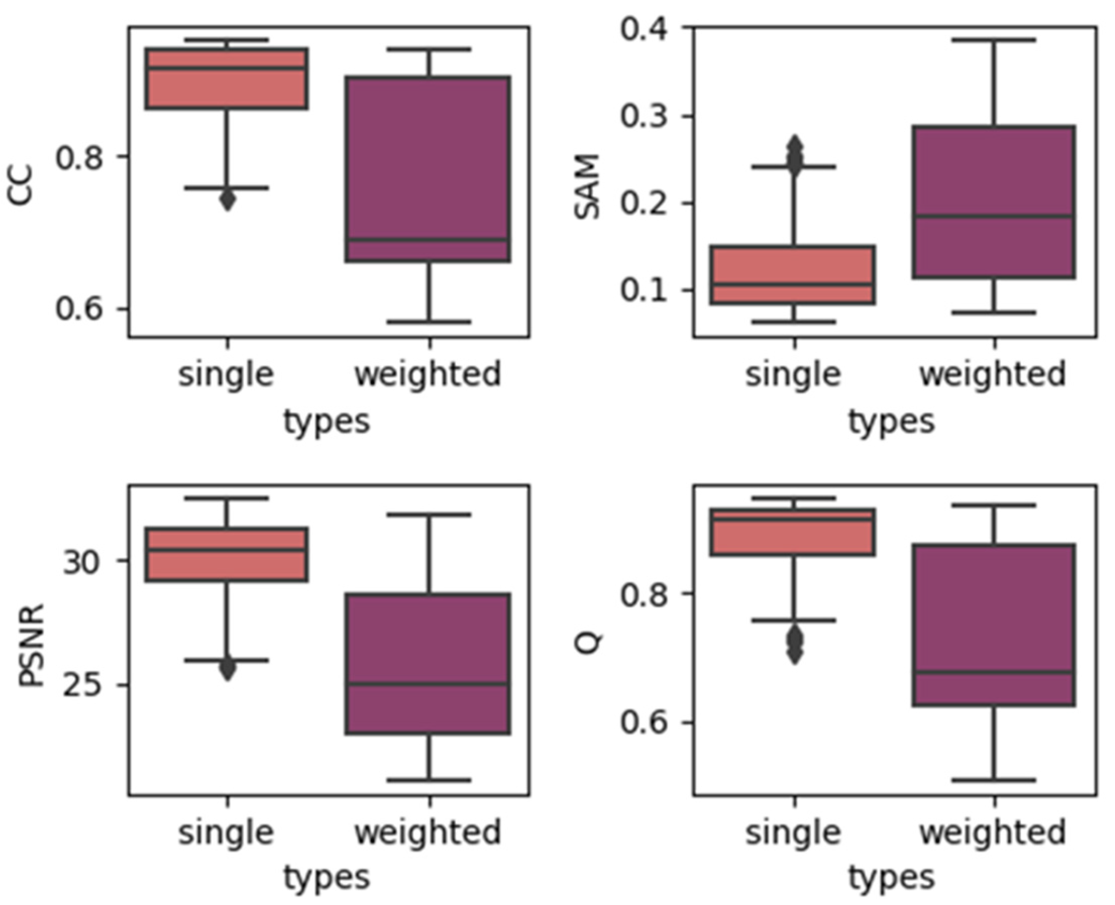
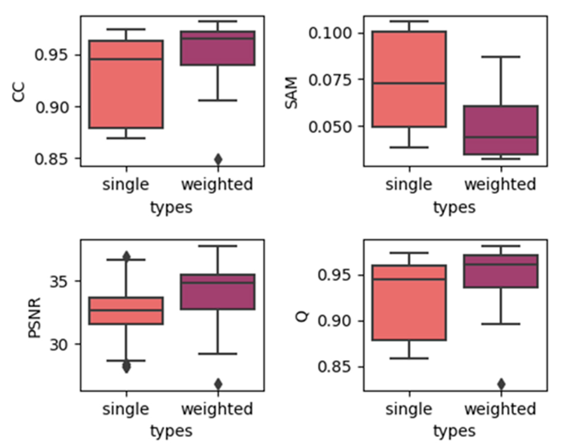
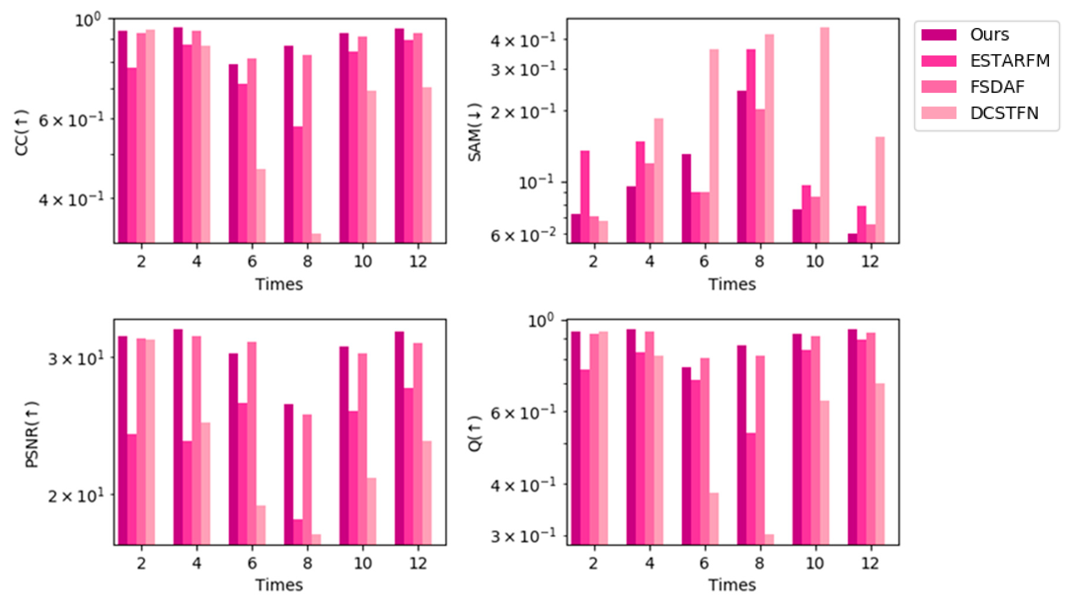
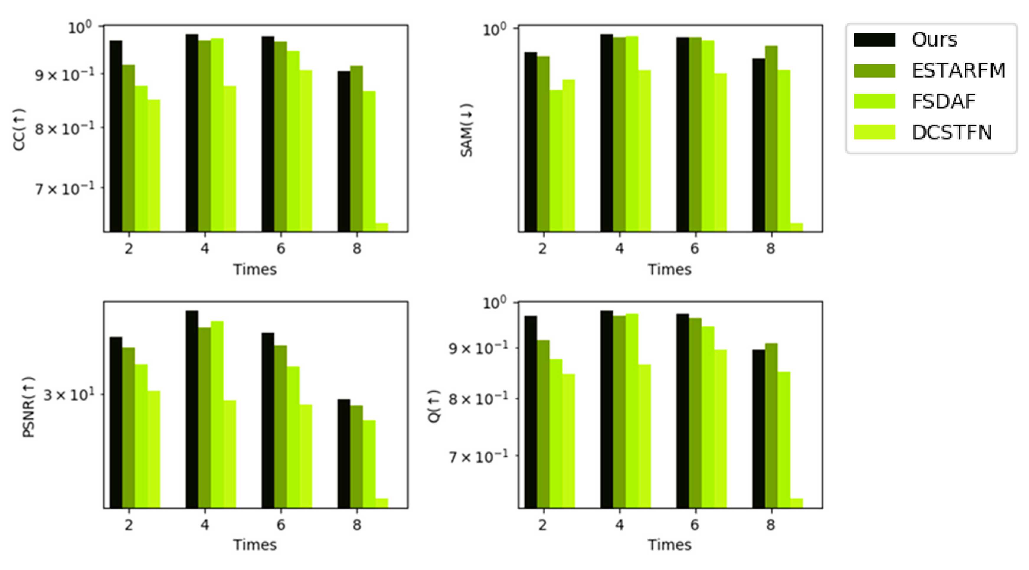
Correlation coefficient (CC) [23]: CC is an important indicator for measuring the relevance between two images. The CC, C C k , for band k can be represented as:
C C k = i = 1 m j = 1 n ( R k ( i , j ) M ( R ) ¯ k ) ( F k ( i , j ) M ( F ) ¯ k ) i = 1 m j = 1 n ( R k ( i , j ) M ( R ) ¯ k ) 2 i = 1 m j = 1 n ( F k ( i , j ) M ( F ) ¯ k ) 2 ,
where R k ( i , j ) represents the pixel value at the k-th band at the (i, j) position of the real reference image, F k ( i , j ) represents the pixel value at the k-th band at the (i, j) position of the fused image and M ( R ) ¯ k and M ( F ) ¯ k respectively, represent the average gray values of the two images in the band k. The closer the CC is to 1, the better relevance between the two images.
(2)
Spectral angle mapper (SAM) [24]: SAM is a common index used to measure the spectral similarity between two spectral vectors or remote sensing images. The SAM of the (i, j)th pixel between the two images is as follows:
θ ( i , j ) = arccos ( R ( i , j ) , F ( i , j ) R ( i , j ) F ( i , j ) ) ,
where R ( i , j ) and F ( i , j ) represent the two spectral vectors of the (i, j)th pixel of the two images, respectively. The smaller the spectral angle, the greater the similarity between the spectra. The perfectly matched spectral angle is 0. For the evaluation of the fusion image, the average spectral angle between the fusion image and the real reference image can be obtained by averaging the spectral angle of every pixel to evaluate the preservation of the spectral characteristics of the fusion image.
(3)
Peak signal-to-noise ratio (PSNR) [25]: PSNR is one of the most commonly used evaluation indices for image fusion evaluation. It evaluates whether the effective information of the fused image is enhanced compared to the original image, and it characterizes the quality of the spatial information reconstruction of the image. The PSNR of band k can be represented as:
P S N R k = 10 log 10 ( m n ( max ( k ) ) 2 / i = 1 m j = 1 n [ R k ( i , j ) F k ( i , j ) ] 2 ) ,
where max ( k ) represents the maximum possible value of the k-th band of the image. The larger the PSNR, the better the quality of the spatial information of the image.
(4)
Universal image quality index (UIQI, Q) [26]: The UIQI is a fusion evaluation index related to the correlation, brightness difference, and contrast difference between images. The formula for calculating the UIQI index of the k-th band of the image before and after fusion is:
U I Q I k = S D ( R F ) k S D ( R ) k S D ( K ) k 2 M ( R ) ¯ k M ( F ) ¯ k [ M ( R ) ¯ k ] 2 + [ M ( F ) ¯ k ] 2 2 S D ( R ) k S D ( K ) k S D ( R ) k 2 + S D ( K ) k 2 ,
where S D ( R F ) k represents the co-standard deviation between the corresponding bands of the two images. The ideal value of UIQI is 1. The closer the index is to 1, the better the fusion effect is.
Among the indices mentioned above, CC and PSNR measure the global fusion accuracies, SAM measures the fusion accuracies in the spectral domain, and UIQI measures the fusion accuracies in the spatial domain. Thus, using the four fusion indices is sufficient for measuring the fusion qualities.

4. Discussion

To test the theory of our method, different parameters and data arrangements were discussed in the ablation study, including the effects of utilizing (1) former prediction and latter prediction with temporal weights, (2) different convolutional layers, and (3) residual blocks (short connection).
As mentioned in Section 2.1, the residual series of MODIS δ C 1 can be arranged by subtracting former subset series from latter subset series, which can be represented as follows:
δ C 1 = C ( t l 1 , x , y , b ) C ( t f 1 , x , y , b ) ,
where C represents the 4D HTLS data, t l 1 { 2 , 4 , , T 1 } , t f 1 { 1 , 3 , , T 2 } , x { 1 , 2 , , W } , y { 1 , 2 , , H } , and b { 1 , 2 , , B } . After mapping to the Landsat residual series and adding the original Landsat series, the reconstructed prediction dataset can be represented as follows:
X 1 = f 1 ( δ C 1 ) + F ( t f 1 , x , y , b ) ,
where f 1 represents the trained residual feature mappings and F represents the 4D HSLT data. The formulas above are for using the predicted images and the images before them to fuse the missing images. Another way is to fuse using the predicted images and the latter images. The residual series δ C 2 is shown as Formula (11) below:
δ C 2 = C ( t l 2 , x , y , b ) C ( t f 2 , x , y , b ) ,
where t f 2 { 2 , 4 , , T 1 } and t l 2 { 3 , 5 , , T } . The final reconstructed prediction dataset is
X 2 = F ( t l 2 , x , y , b ) f 2 ( δ C 2 ) ,
where f 2 represents the trained residual feature mappings. Thus, we obtain two results, X 1 and X 2 , based on the different residual series.
Here, we introduce the temporal weight to combine these two results, and the weights are larger when the dates are close together. The temporal weight calculation can be represented as follows:
X = X 1 d 1 + X 2 d 2 1 d 1 + 1 d 2 ,
where d 1 and d 2 represent the vectors of time intervals for the left and right dates of the prediction dates respectively, and can be calculated as
d 1 = t l 1 t f 1 ,   d 2 = t f 2 t l 2 .
For three datasets, we set the depth of the network as 3 to 9, and each experiment yields two results using the single-date prediction (Formulas (9) and (10)) and the temporal weighted prediction (Formulas (9)–(14)). We also set experiments utilizing two residual blocks on three datasets. The number of experiments is 45 in total.

4.1. Effects of Utilizing Temporal Weights

In order to show the overall effect of utilizing temporal weights, we used the results of two temporal strategies, which contain the results of models with all depths, to construct a boxplot to show the effect of utilizing temporal weights. The results are produced by grouping the single-date prediction results together regardless of the depths or dates of images. The results for three different datasets are shown in Figure 4, Figure 5 and Figure 6. In each subplot, the x-axis represents the weight strategy and the y-axis represents the different fusion indices. As shown in Figure 4 and Figure 5, the results of the CIA and LGC datasets have the same tendency: the temporal weighted results are worse than the single-date prediction results across all the fusion quality indices. Additionally, the ranges of the temporal weighted results are larger than those of the single-date results. The more abrupt or unpredictable the change in the dataset, the more obvious the tendency (judging by boxplot ranges and averages). However, for the RDT, the temporal weighted prediction yielded better results, with smaller ranges, compared with the single-date prediction. The reason for this may be that, when the landcover undergoes abrupt or irregular changes, the temporal weight strategy averages the abrupt changes, decreasing the accuracy, but when the landcovers change regularly, the temporal weights combine the changes to obtain the results. Thus, this method may depend highly on landcover changes. However, for the three datasets, the characteristics of the outliers are the same. The outliers of the single-date results are close to the maximum/minimum of the boxplot, yet the outliers of the temporal weighted results are far away from the maximum/minimum of the boxplot. This may indicate that the temporal weighted method may cause some uncertainties.

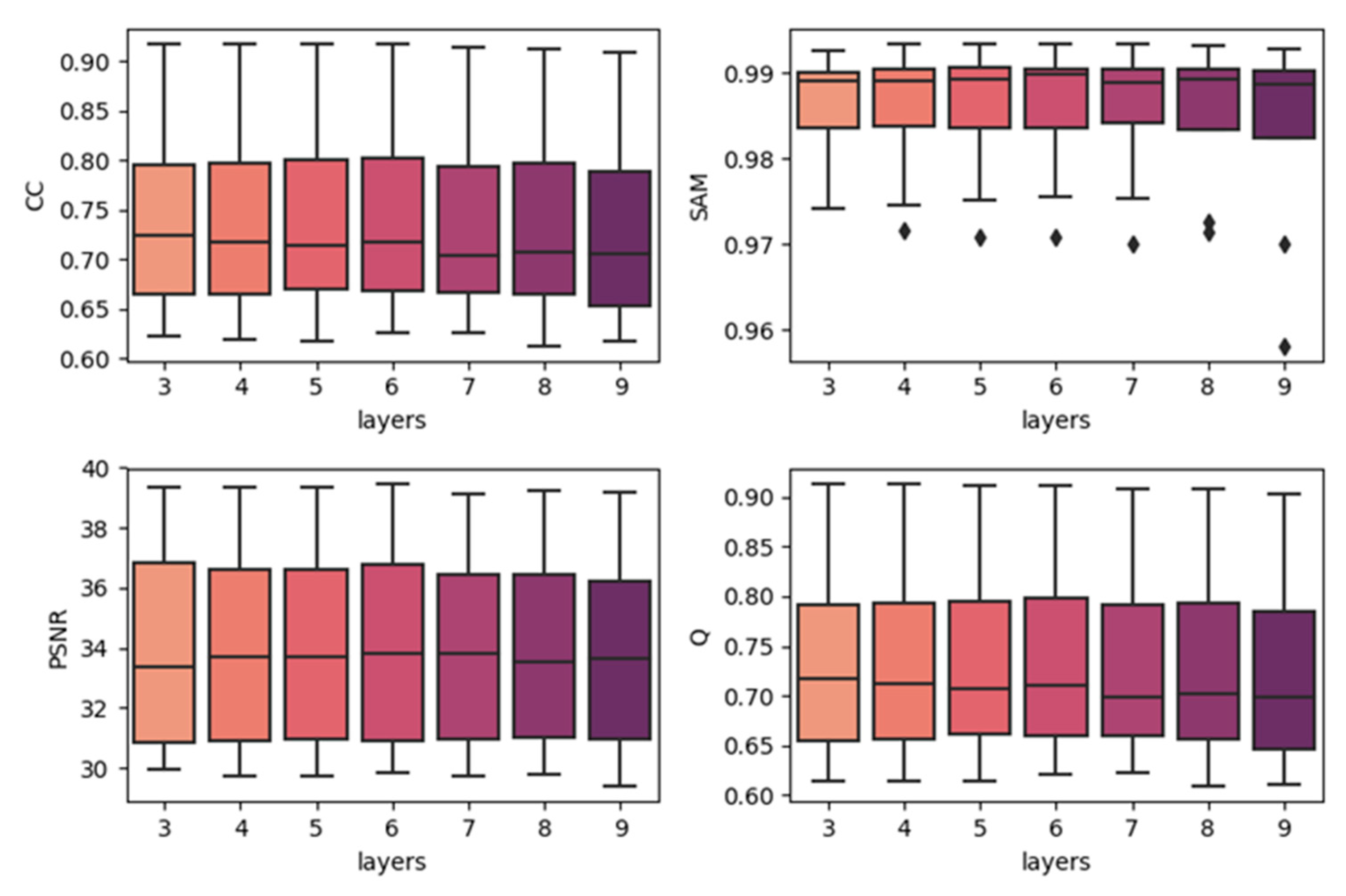
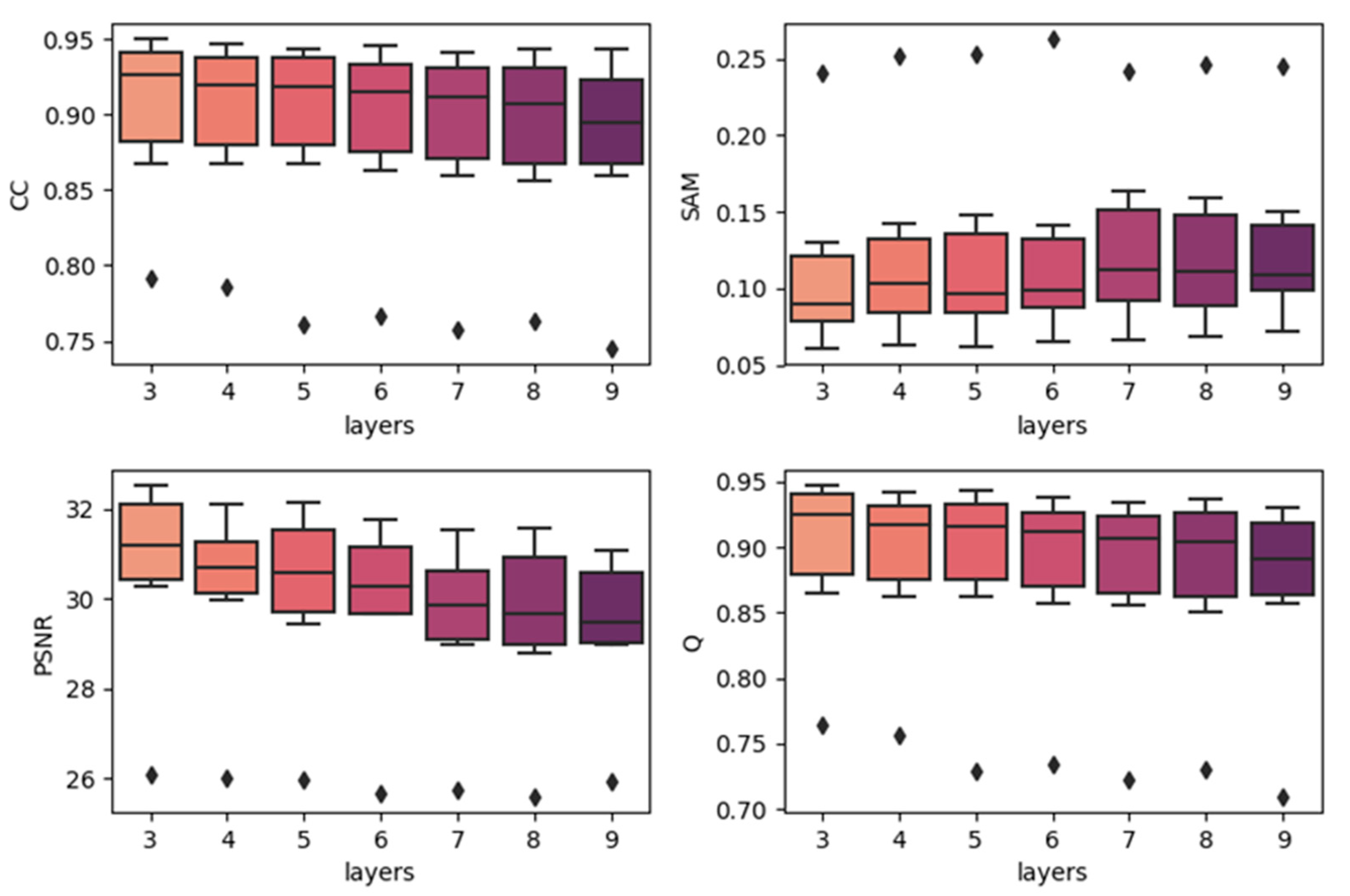
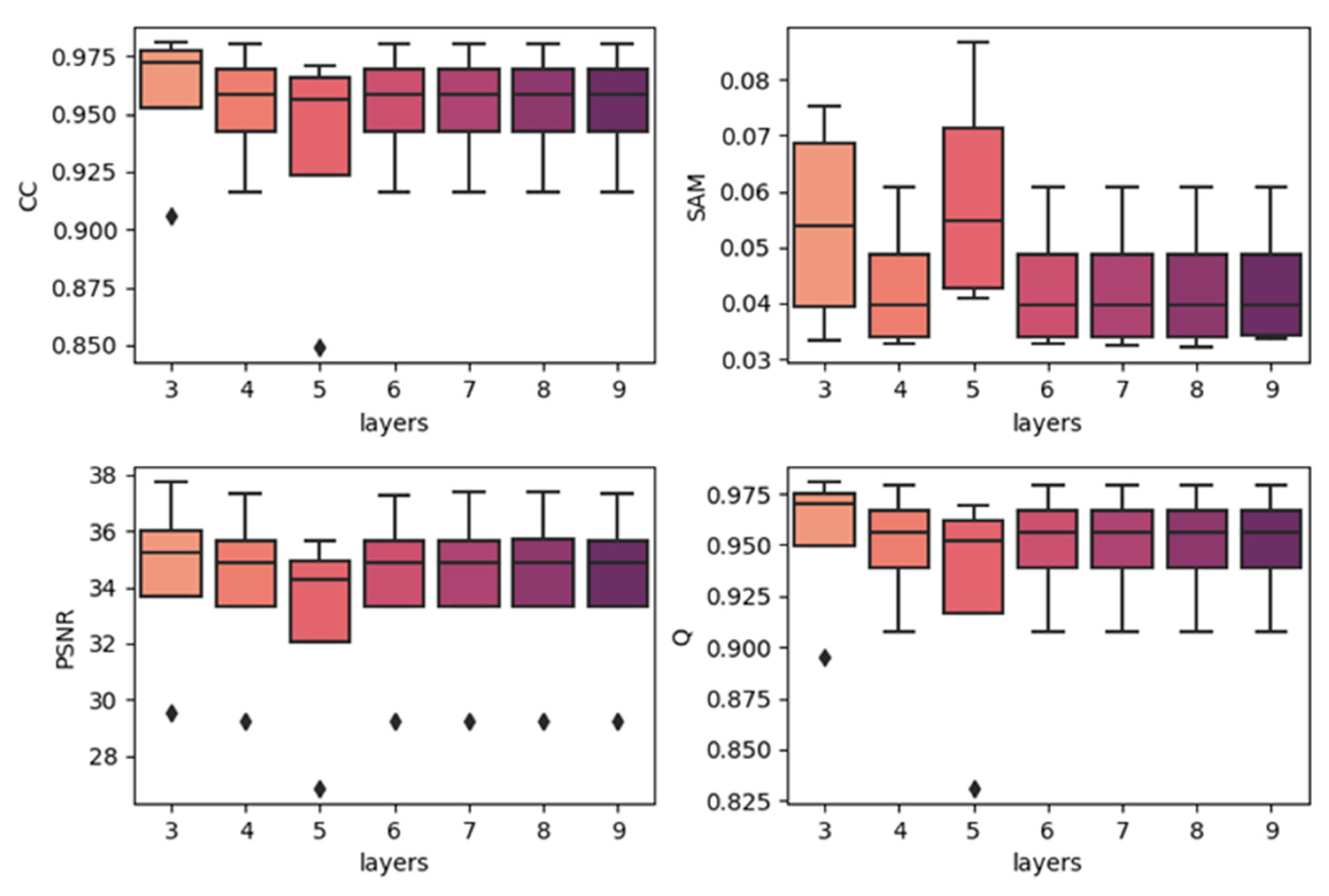
4.2. Effects of Network Depth

To show the effects of network depth, we generated boxplots of experiments with different network depths. The results are produced by combining the results of the same depth together with the best temporal strategy, regardless of the predicted dates. The results are shown in Figure 7, Figure 8 and Figure 9. In each subplot, the x-axis indicates the depth (layers) of the utilized model, and the y-axis represents the values of the different fusion indices. In the three datasets, increasing the model’s depth did not increase the accuracy. In the CIA and LGC datasets, the accuracy decreases when the depth increases. As the depth increases, the outliers become more distant from the other values. In the RDT datasets, although the tendency was not very clear, as the depth increases, the accuracies do not significantly increase. The outliers do not show the same tendency with CIA and LGC, and this may be due to the reason mentioned in Section 4.1: the temporal weighted strategy may cause some uncertainties in certain points. Since the computational cost and running time increase when the depth of the model increases, three-layer fully convolutional networks are the best choice for our method. It is not worth the cost to use more layers, particularly for the architecture with residual series. This may be due to the reason that the features of the residual series are not obvious and it is easy to cause overfitting. As the depth increases, it becomes easier to learn the mappings too delicately.

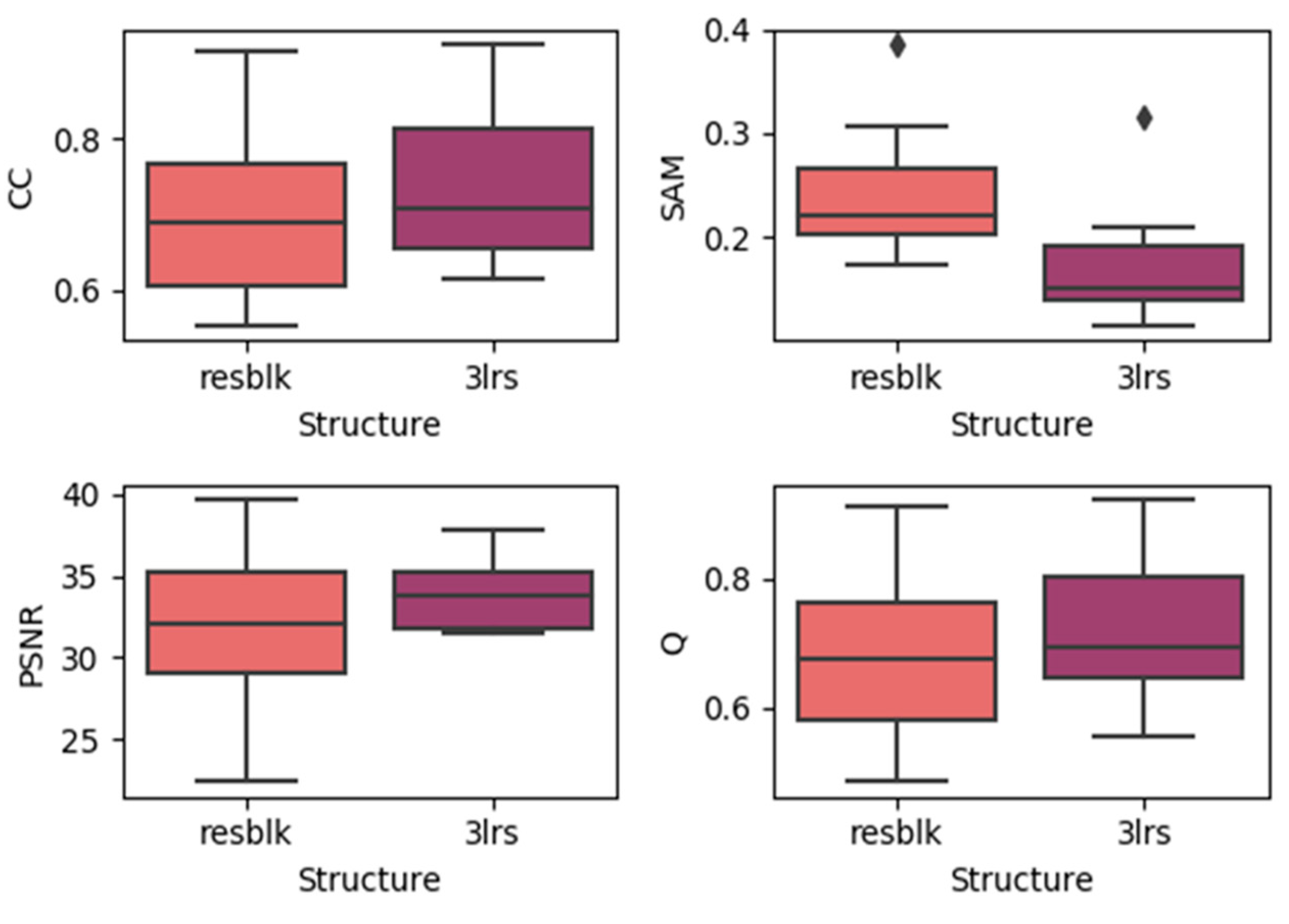
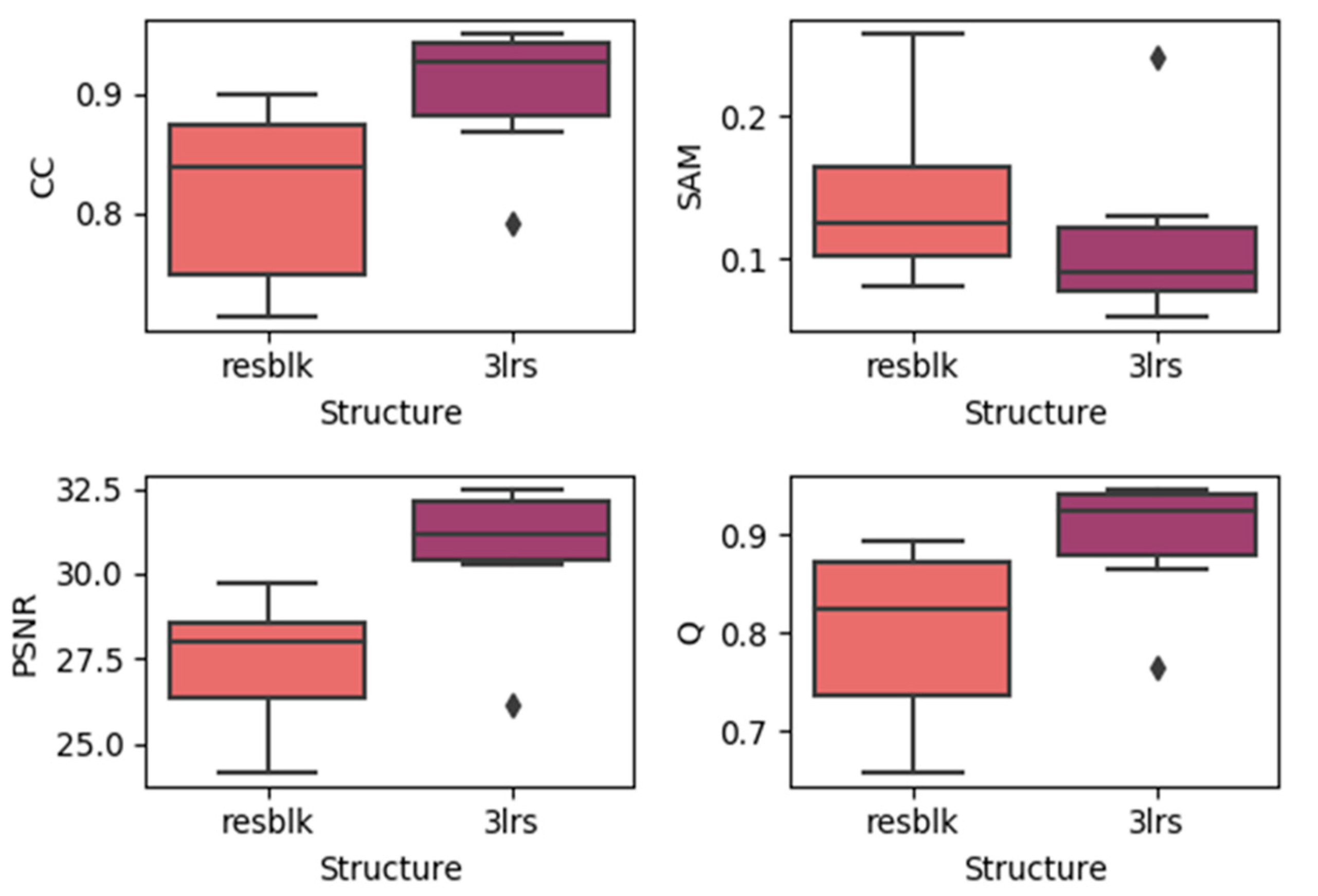
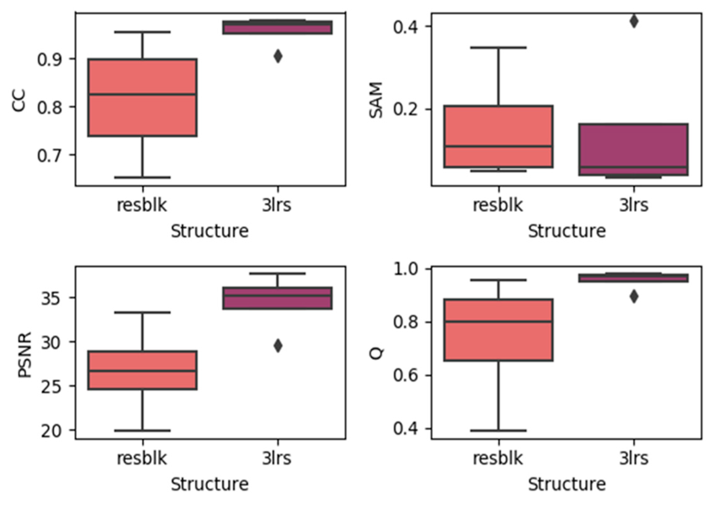
4.3. Effects of Utilizing Residual Blocks

Piling a greater number of convolutional network layers makes it easy for the model to encounter a vanishing gradient. The idea of residual networks is proposed to deal with the difficulty of training deeper networks. The purpose is to learn the residuals of two CNN layers to overcome redundancy and a vanishing gradient. As the accuracy of our model decreases when the layer count increases, we attempted to utilize residual blocks to determine whether the accuracy could be increased. The architecture is shown in the graph in Figure 10.
Here, we generated boxplots of experiments on the three datasets with residual blocks and three-layer networks (regardless of the prediction dates), which are presented in the Figure 11, Figure 12 and Figure 13. In each subplot, the x-axis represents the utilized model with the residual block (noted as resblk) and the model with three convolutional neural network layers (3lrs). The y-axis indicates the values for different validation indices. With all the datasets, utilizing residual blocks did not increase the accuracy and instead decreased the average accuracy as well as further increasing the divergence in the results. In addition, as the residual blocks were utilized, the processing time was increased. This may be due to the fact that, in a more sophisticated model, it is easier to cause overfitting when the feature is not obvious.

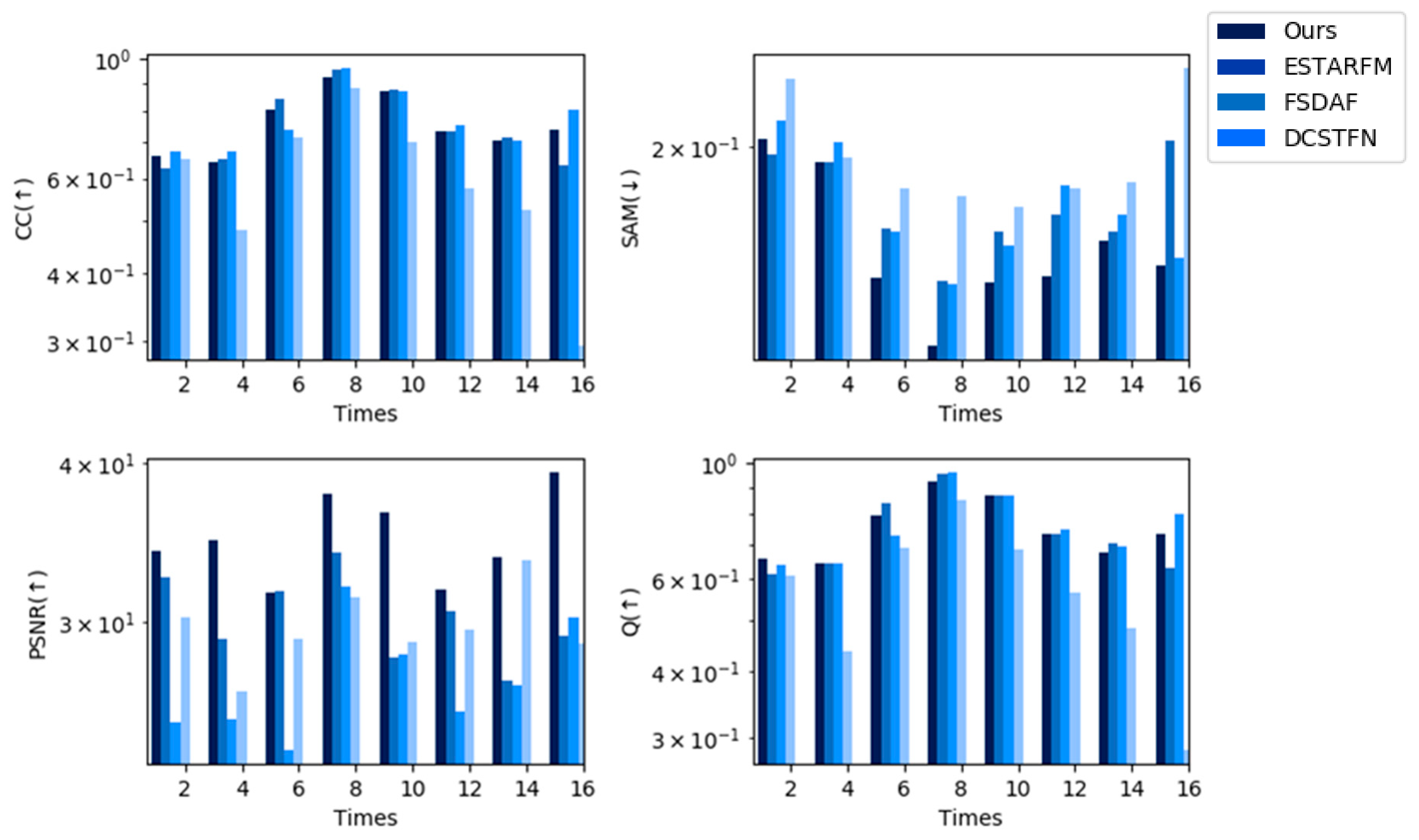
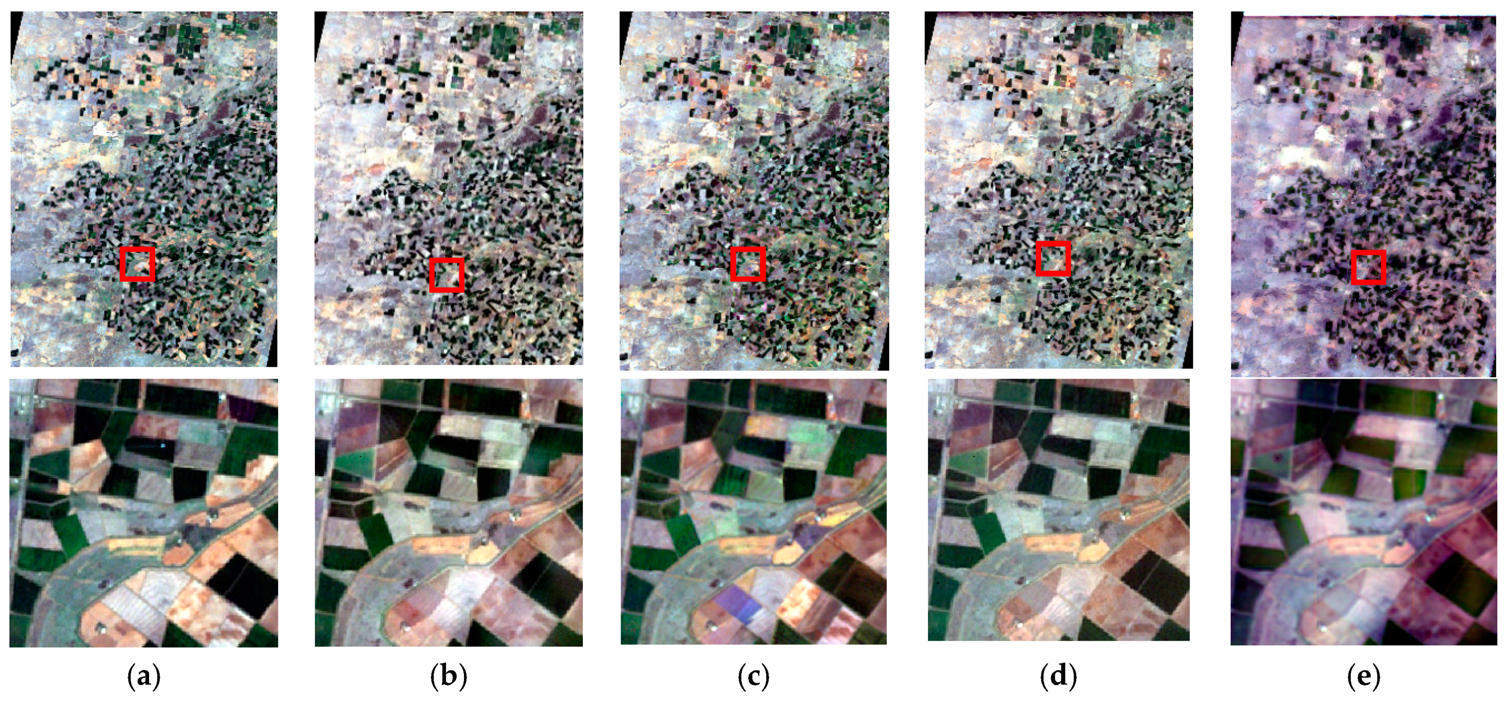
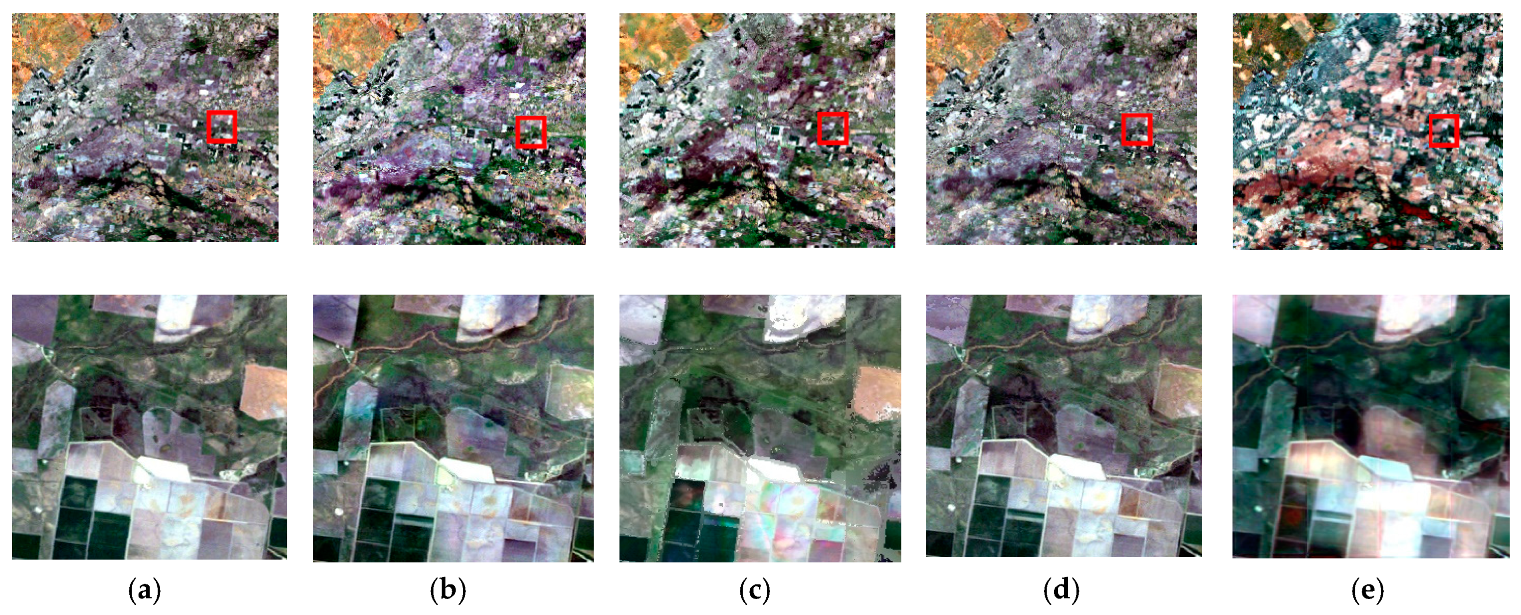
4.4. Comparison with State-of-the-Art Spatiotemporal Fusion Methods

The goal of our method is to increase the efficiency while ensuring that the accuracy is maintained in comparison with existing spatiotemporal fusion methods. To verify whether our goals were achieved, we chose the best result from our experiments and compared it with the existing spatiotemporal fusion methods of ESTARFM, FSDAF, and DCSTFN. ESTARFM and FSDAF are traditional spatiotemporal fusion methods, while DCSTFN is a deep learning-based spatiotemporal method using 2D CNNs. For ESTARFM, we used the fast version, with the window size set to 25, the estimated number of classes set to 4, and the patch size set to 500. For FSDAF, we also used the fast version, with the window size set to 25, the estimated number of classes set to 4, and the patch size set to 50. For DCSTFN, we trained the model using Landsat and MODIS on the same date and predicted the missing Landsat images: the number of epochs was set to 100, the optimizer was Adam, the learning rate was set to the default as 0.001, and the patch size was set to 64. We measured the accuracy of each method using the nine indices and recorded the running time for the entire long time-series dataset.
Figure 14, Figure 15 and Figure 16 show bar charts of the four indices for each method. For each subplot, the x-axis represents the dates indexed in chronological order and the y-axis represents the different fusion indices. Experiments on the CIA dataset show that the CC and Q were slightly lower for our method than for the other methods from a general perspective, but were not the lowest in all experiments; however, our method performed the best in terms of the other indices among all spatiotemporal fusion methods used in the experiments from a general perspective. For the SAM and PSNR, our method performed the best in seven predictions. Experiments on the LGC dataset show that for the CC, PSNR, and Q, our method outperforms other methods in five predictions. For SAM, the results of our methods are slightly poor yet still not the worst among all the methods in the experiment. Experiments on the RDT dataset indicate that our method yields the best results.
To compare the texture and tones of the reconstructed dataset, we chose one date of each dataset to display the fusion results of the whole scene in detail. For the CIA dataset, the 10th date was selected, and the RGB composites are shown in Figure 17. Our method showed a good recovery of the texture and tone similar to that of the FSDAF. As seen in the results of the ESTARFM, some landcovers were mis-predicted. The DCSTFN recovered the data but suffered from blur. Thus, for the CIA dataset, our method and the FSDAF predicted the missing image best.
In the LGC dataset, the 10th date was selected, which was the date that the flood occurred, causing drastic change. The RGB composites are shown in Figure 18. Our method was able to recover the flooded area with an accurate texture and tone. The FSDAF could also well-predict the flooded area and seemed to outperform the ESTARFM. With the DCSTFN, the tones were slightly different from the reference image and the texture suffered from blur.
In the RDT dataset, the 6th date was selected, and the RGB composites are shown in Figure 19. In the overall and detailed images (with multiple landcover types), our method performed well, as did the FSDAF. The tone was not completely true to the original when using the DCSTFN and ESTARFM.
To present the average accuracies of our methods, we calculated the average indices of each method on all dates and recorded the overall running times of all datasets. The average accuracies and total running times are shown in Table 4 and Table 5. For all the fusion indices, the performance of the STF3DCNN was the best among the four methods. Most importantly, the total running time was significantly decreased. Compared with traditional methods using a central processing unit, our method was able to decrease the running time by 109 times (ESTARFM) and 104 times (FSDAF). Compared with the DCSTFN, a deep learning spatiotemporal fusion method, the average running time decreased 12-fold among three datasets. We also observed the tendency of a higher efficiency with larger datasets. The experiments demonstrated that the STF3DCNN successfully maintains the average accuracy of the existing methods, while, at the same time, significantly increasing the efficiency.

5. Conclusions

We proposed a fast spatiotemporal fusion method using 3D fully convolutional networks (STF3DCNN) on a spatial-temporal-spectral dataset. The long time-series data were arranged and operated four-dimensionally in a spatial-temporal-spectral dataset based on the idea of an MDD. By learning the mappings between residual series of HTLS and HSLT datasets using 3D fully convolutional networks, the model can restore the 4D HSHT dataset with a high efficiency compared with existing methods, while maintaining the accuracy.
We used three datasets to verify the efficiency and accuracy of our method. An ablation study was performed to discuss the effects of parameters on long time-series spatiotemporal fusion on different occasions, including network depth, the use of temporal weights, and the use of residual blocks. Fewer layers resulted in a better accuracy and increased efficiency. Temporal weights improved the model performance for landcover with regular seasonal changes, but not for landcover with sudden irregular changes, and utilizing residual blocks did not increase the accuracy. Finally, our method was compared with existing methods in terms of accuracy and running time. Our method can highly improve the efficiency while maintaining its overall accuracy, especially in the case of very large datasets covering long time periods.

Author Contributions

Conceptualization, L.Z., M.P. and X.S.; methodology, M.P.; software, M.P.; validation, M.P.; formal analysis, M.P.; investigation, M.P.; resources, L.Z., X.S. and Y.C.; data curation, M.P.; writing—original draft preparation, M.P.; writing—review and editing, L.Z. and M.P.; visualization, M.P. and X.Z.; supervision, L.Z.; project administration, L.Z. and X.S.; funding acquisition, L.Z. All authors have read and agreed to the published version of the manuscript.

Funding

This research was funded by the National Natural Science Foundation of China, grant number 41830108,41701404, the National Key R&D Program of China, grant number 2017YFC1500900, XPCC major science and technology projects, grant number 2018AA004, and XPCC innovation team in key areas, grant number 2018CB004.

Acknowledgments

The authors would like to thank anonymous reviewers for their great comments and suggestions.

Conflicts of Interest

The authors declare no conflict of interest.

References

  1. Zhang, L.; Peng, M.; Sun, X.; Cen, Y.; Tong, Q. Progress and bibliometric analysis of remote sensing data fusion methods (1992–2018). J. Remote Sens. 2019, 23, 1993–2002. [Google Scholar] [CrossRef]
  2. Gao, F.; Masek, J.; Schwaller, M.; Hall, F. On the blending of the Landsat and MODIS surface reflectance: Predicting daily Landsat surface reflectance. IEEE Trans. Geosci. Remote Sens. 2006, 44, 2207–2218. [Google Scholar]
  3. Hilker, T.; Wulder, M.A.; Coops, N.C.; Linke, J.; Mcdermid, G.; Masek, J.G.; Gao, F.; White, J.C. A new data fusion model for high spatial- and temporal-resolution mapping of forest disturbance based on Landsat and MODIS. Remote Sens. Environ. 2009, 113, 1613–1627. [Google Scholar] [CrossRef]
  4. Zhu, X.; Jin, C.; Feng, G.; Chen, X.; Masek, J.G. An enhanced spatial and temporal adaptive reflectance fusion model for complex heterogeneous regions. Remote Sens. Environ. 2010, 114, 2610–2623. [Google Scholar] [CrossRef]
  5. Fu, D.; Chen, B.; Wang, J.; Zhu, X.; Hilker, T. An Improved Image Fusion Approach Based on Enhanced Spatial and Temporal the Adaptive Reflectance Fusion Model. Remote Sens. 2013, 5, 6346–6360. [Google Scholar] [CrossRef] [Green Version]
  6. Wang, J.; Huang, B. A Rigorously-Weighted Spatiotemporal Fusion Model with Uncertainty Analysis. Remote Sens. 2017, 9, 990. [Google Scholar] [CrossRef] [Green Version]
  7. Zhukov, B.; Oertel, D.; Lanzl, F.; Reinhackel, G. Unmixing-based multisensor multiresolution image fusion. IEEE Trans. Geosci. Remote Sens. 1999, 37, 1212–1226. [Google Scholar] [CrossRef]
  8. Zhu, X.; Helmer, E.H.; Gao, F.; Liu, D.; Chen, J.; Lefsky, M.A. A flexible spatiotemporal method for fusing satellite images with different resolutions. Remote Sens. Environ. 2016, 172, 165–177. [Google Scholar] [CrossRef]
  9. Mingquan, W.; Zheng, N.; Changyao, W.; Chaoyang, W.; Li, W. Use of MODIS and Landsat time series data to generate high-resolution temporal synthetic Landsat data using a spatial and temporal reflectance fusion model. J. Appl. Remote Sens. 2012, 6, 063507. [Google Scholar] [CrossRef]
  10. Zhang, W.; Li, A.; Jin, H.; Bian, J.; Zhengjian, Z.; Lei, G.; Qin, Z.; Huang, C. An Enhanced Spatial and Temporal Data Fusion Model for Fusing Landsat and MODIS Surface Reflectance to Generate High Temporal Landsat-Like Data. Remote Sens. 2013, 5, 5346–5368. [Google Scholar] [CrossRef] [Green Version]
  11. Wu, P.; Shen, H.; Zhang, L.; Gottsche, F.M. Integrated fusion of multi-scale polar-orbiting and geostationary satellite observations for the mapping of high spatial and temporal resolution land surface temperature. Remote Sens. Environ. 2015, 156, 169–181. [Google Scholar] [CrossRef]
  12. Amorós-López, J.; Gómez-Chova, L.; Alonso, L.; Guanter, L.; Zurita-Milla, R.; Moreno, J.; Camps-Valls, G. Multitemporal fusion of Landsat/TM and ENVISAT/MERIS for crop monitoring. Int. J. Appl. Earth Obs. Geoinf. 2013, 23, 132–141. [Google Scholar] [CrossRef]
  13. Lu, M.; Chen, J.; Tang, H.; Rao, Y.; Yang, P.; Wu, W. Land cover change detection by integrating object-based data blending model of Landsat and MODIS. Remote Sens. Environ. 2016, 184, 374–386. [Google Scholar] [CrossRef]
  14. Moosavi, V.; Talebi, A.; Mokhtari, M.H.; Shamsi, S.R.F.; Niazi, Y. A wavelet-artificial intelligence fusion approach (WAIFA) for blending Landsat and MODIS surface temperature. Remote Sens. Environ. 2015, 169, 243–254. [Google Scholar] [CrossRef]
  15. Song, H.; Liu, Q.; Wang, G.; Hang, R.; Huang, B. Spatiotemporal Satellite Image Fusion Using Deep Convolutional Neural Networks. IEEE J. Sel. Top. Appl. Earth Obs. Remote Sens. 2018, 11, 821–829. [Google Scholar] [CrossRef]
  16. Tan, Z.; Peng, Y.; Di, L.; Tang, J. Deriving High Spatiotemporal Remote Sensing Images Using Deep Convolutional Network. Remote Sens. 2018, 10, 1066. [Google Scholar] [CrossRef] [Green Version]
  17. Zhang, L.; Chen, H.; Sun, X.; Fu, D.; Tong, Q. Designing spatial-temporal-spectral integrated storage structure of multi-dimensional remote sensing images. Yaogan Xuebao J. Remote Sens. 2017, 21, 62–73. [Google Scholar] [CrossRef]
  18. Tran, D.; Bourdev, L.; Fergus, R.; Torresani, L.; Paluri, M. Learning Spatiotemporal Features with 3D Convolutional Networks. In Proceedings of the 2015 IEEE International Conference on Computer Vision (ICCV), Santiago, Chile, 7–13 December 2015; pp. 4489–4497. [Google Scholar]
  19. Sebastianelli, A.; Del Rosso, M.P.; Ullo, S. Automatic Dataset Builder for Machine Learning Applications to Satellite Imagery; 2020. Available online: https://arxiv.org/abs/2008.01578 (accessed on 18 September 2020).
  20. Sun, Z.; Wang, J.; Lei, P.; Qin, Z. Multiple Walking People Classification with Convolutional Neural Networks Based on Micro-Doppler. In Proceedings of the 2018 10th International Conference on Wireless Communications and Signal Processing (WCSP), Hangzhou, China, 18–20 October 2018; pp. 1–4. [Google Scholar]
  21. Emelyanova, I.V.; McVicar, T.R.; Van Niel, T.G.; Li, L.T.; van Dijk, A.I.J.M. Assessing the accuracy of blending Landsat–MODIS surface reflectances in two landscapes with contrasting spatial and temporal dynamics: A framework for algorithm selection. Remote Sens. Environ. 2013, 133, 193–209. [Google Scholar] [CrossRef]
  22. Salomonson, V.V.; Guenther, B.; Masuoka, E. A summary of the status of the EOS Terra mission Moderate Resolution Imaging Spectroradiometer (MODIS) and attendant data product development after one year of on-orbit performance. In Proceedings of the Scanning the Present and Resolving the Future, Proceedings. IEEE 2001 International Geoscience and Remote Sensing Symposium (Cat. No.01CH37217), Sydney, Australia, 9–13 July 2001; Volume 1193, pp. 1197–1199. [Google Scholar]
  23. Alparone, L.; Wald, L.; Chanussot, J.; Thomas, C.; Gamba, P.; Bruce, L. Comparison of Pansharpening Algorithms: Outcome of the 2006 GRS-S Data Fusion Contest. IEEE Trans. Geosci. Remote Sens. 2007, 45, 3012–3021. [Google Scholar] [CrossRef] [Green Version]
  24. Zhang, Y.; De Backer, S.; Scheunders, P. Noise-Resistant Wavelet-Based Bayesian Fusion of Multispectral and Hyperspectral Images. IEEE Trans. Geosci. Remote Sens. 2009, 47, 3834–3843. [Google Scholar] [CrossRef]
  25. Huynh-Thu, Q.; Ghanbari, M. Scope of validity of PSNR in image/video quality assessment. Electron. Lett. 2008, 44, 800–801. [Google Scholar] [CrossRef]
  26. Dan, L.; Hao, M.; Zhang, J.Q.; Bo, H.; Lu, Q. A universal hypercomplex color image quality index. In Proceedings of the IEEE Instrumentation & Measurement Technology Conference, Graz, Austria, 13–16 May 2012. [Google Scholar]
Figure 1. Temporal Interleaved by Pixel (TIP) data format of the multi-dimensional dataset.
Remotesensing 12 03888 g001
Figure 2. Training stage of the fast three-dimensional convolutional neural network-based spatiotemporal fusion method (STF3DCNN).
Remotesensing 12 03888 g002
Figure 3. Predicting stage of the fast three-dimensional convolutional neural network-based spatiotemporal fusion method (STF3DCNN).
Remotesensing 12 03888 g003
Figure 4. Results of using single/weighted double images in the CIA dataset.
Remotesensing 12 03888 g004
Figure 5. Results of using single/weighted double images in the LGC dataset.
Remotesensing 12 03888 g005
Figure 6. Results of using single/weighted double images in the RDT dataset.
Remotesensing 12 03888 g006
Figure 7. Results of using different network depths in the CIA dataset (single-date prediction).
Remotesensing 12 03888 g007
Figure 8. Results of using different network depths in the LGC dataset (single-date prediction).
Remotesensing 12 03888 g008
Figure 9. Results of using different network depths in the RDT (weighted date prediction).
Remotesensing 12 03888 g009
Figure 10. Residual blocks implemented in the mapping model.
Remotesensing 12 03888 g010
Figure 11. Results of using residual blocks in the CIA dataset.
Remotesensing 12 03888 g011
Figure 12. Results of using residual blocks in the LGC dataset.
Remotesensing 12 03888 g012
Figure 13. Results of using residual blocks in the RDT dataset.
Remotesensing 12 03888 g013
Figure 14. Indices using the CIA dataset (STF3DCNN, ESTARFM, FSDAF, DCSTFN).
Remotesensing 12 03888 g014
Figure 15. Indices using the LGC dataset (STF3DCNN, ESTARFM, FSDAF, DCSTFN).
Remotesensing 12 03888 g015
Figure 16. Indices using the RDT (STF3DCNN, ESTARFM, FSDAF, DCSTFN).
Remotesensing 12 03888 g016
Figure 17. RGB composites (Red-Band 3, Green-Band 2, Blue- Band 1) of the results of the CIA dataset on date 10 (overall and in detail): (a) reference image, (b) STF3DCNN, (c) ESTARFM, (d) FSDAF, and (e) DCSTFN.
Remotesensing 12 03888 g017
Figure 18. RGB (Red-Band 3, Green-Band 2, Blue- Band 1) composites of the results of the LGC dataset on date 10 (overall and in detail): (a) reference image, (b) STF3DCNN, (c) ESTARFM, (d) FSDAF, and (e) DCSTFN.
Remotesensing 12 03888 g018
Figure 19. RGB (Red-Band 4, Green-Band 3, Blue- Band 2) composites of the results of the LGC dataset on date 10 (overall and in detail): (a) reference image, (b) STF3DCNN, (c) ESTARFM, (d) FSDAF, and (e) DCSTFN.
Remotesensing 12 03888 g019
Table 1. Spatiotemporal fusion methods mentioned in the article.
CategoriesSub-CategoriesRepresentative Methods
Weight function methodsSTARFM, ESTARFM, mESTARFM, RWSTFM
Linear optimization decomposition methodsSpectral-unmixing methodMMT, STDFM, enhanced STDFM, soft clustering, OBIA
Bayesian method
Sparse representation method
Nonlinear optimization methodsANN, DCSTFN, STFDCNN
Table 2. Acquisition dates of datasets of CIA, LGC, and RDT.
CIALGCRDT
Image #DateIntervalsImage #DateIntervalsImage #DateIntervals
18-Oct-2001 116-Apr-2004 13-Jun-2013
217-Oct-2001922-May-200416219-Jun-201316
32-Nov-20011635-Jul-20046435-Jul-201316
49-Nov-2001746-Aug-200432421-Jul-201316
525-Nov-200116522-Aug-200416522-Aug-201332
64-Dec-20019625-Oct-20046467-Sep-201316
75-Jan-200232726-Nov-200432723-Sep-201316
812-Jan-20027812-Dec-20041689-Oct-201316
913-Feb-200232928-Dec-200416925-Oct-201316
1022-Feb-200291013-Jan-200516
1110-Mar-2002161129-Jan-200516
1217-Mar-200271214-Feb-200516
132-Apr-200216132-Mar-200516
1411-Apr-20029143-Apr-0532
1518-Apr-20027
1627-Apr-20029
174-May-20027
1 Image # represents the sequence number of the images in the dataset.
Table 3. Band information of datasets CIA, LGC, and RDT.
CIALGCRDT
Band NamesWavelengthsBand NamesWavelengthsBand NamesWavelengths
Band 1 Visible0.45–0.52 µmBand 1 Visible0.45–0.52 µmBand 2 Visible0.450–0.51 µm
Band 2 Visible0.52–0.60 µmBand 2 Visible0.52–0.60 µmBand 3 Visible0.53–0.59 µm
Band 3 Visible 0.63–0.69 µmBand 3 Visible0.63–0.69 µmBand 4 Red 0.64–0.67 µm
Band 4 Near-Infrared0.77–0.90 µmBand 4 Near-Infrared0.76–0.90 µmBand 5 Near-Infrared0.85–0.88 µm
Band 5 Short-wave Infrared1.55–1.75 µmBand 5 Near-Infrared1.55–1.75 µm
Band 7 Mid-Infrared2.08–2.35 µmBand 7 Mid-Infrared2.08–2.35 µm
Table 4. Average fusion indices of the three datasets.
CC (↑)SAM (↓)PSNR (↑)Q (↑)
STF3DCNN0.87400.120133.37090.8684
ESTARFM0.8255 0.147129.2558 0.8158
FSDAF0.8595 0.1266 29.9007 0.8525
DCSTFN0.6969 0.2227 26.8396 0.6715
1 Bold values represent the best performance.
Table 5. Running times 1 of the entire time series using different methods.
CIALGCRDT
STF3DCNN55298777
ESTARFM65,871.94109,361.79514,435.744
FSDAF27,626.01751,858.2987595.211
DCSTFN691012,278489.4740
1 Times are expressed in seconds.
Publisher’s Note: MDPI stays neutral with regard to jurisdictional claims in published maps and institutional affiliations.

