Impact of Three Gorges Reservoir Water Impoundment on Vegetation–Climate Response Relationship


Abstract
1. Introduction
2. Data and Methods
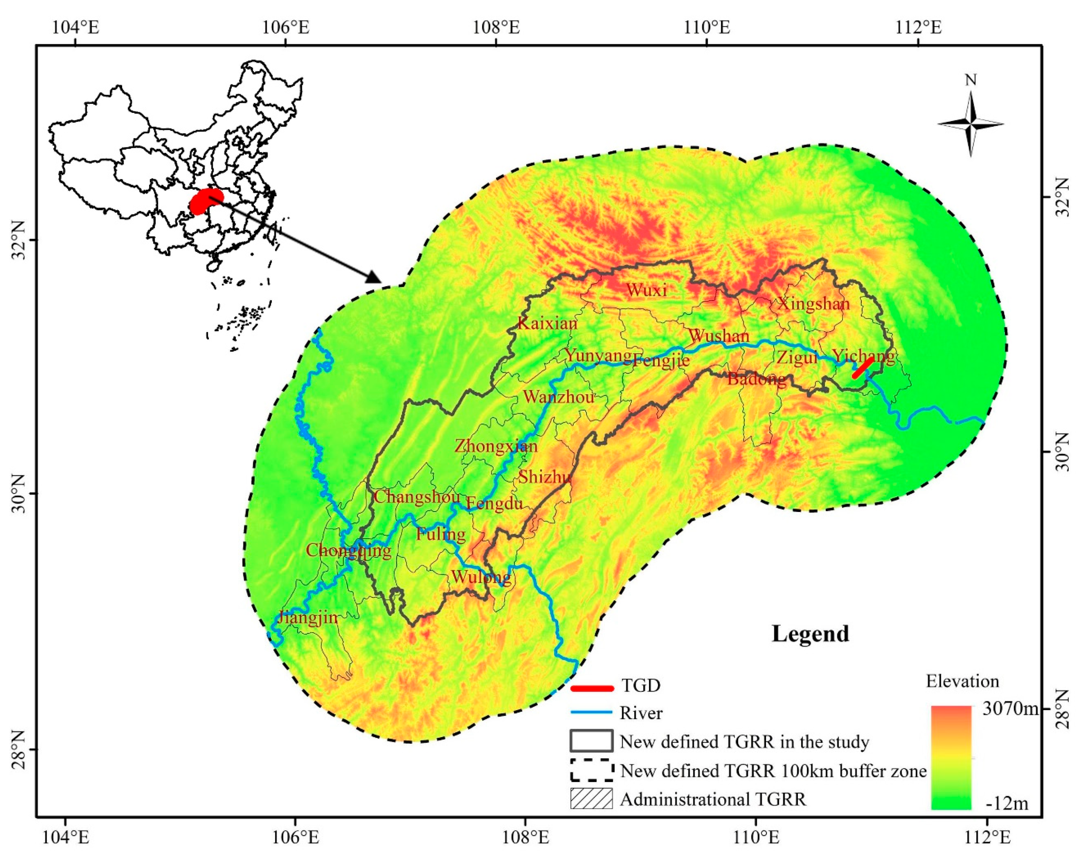
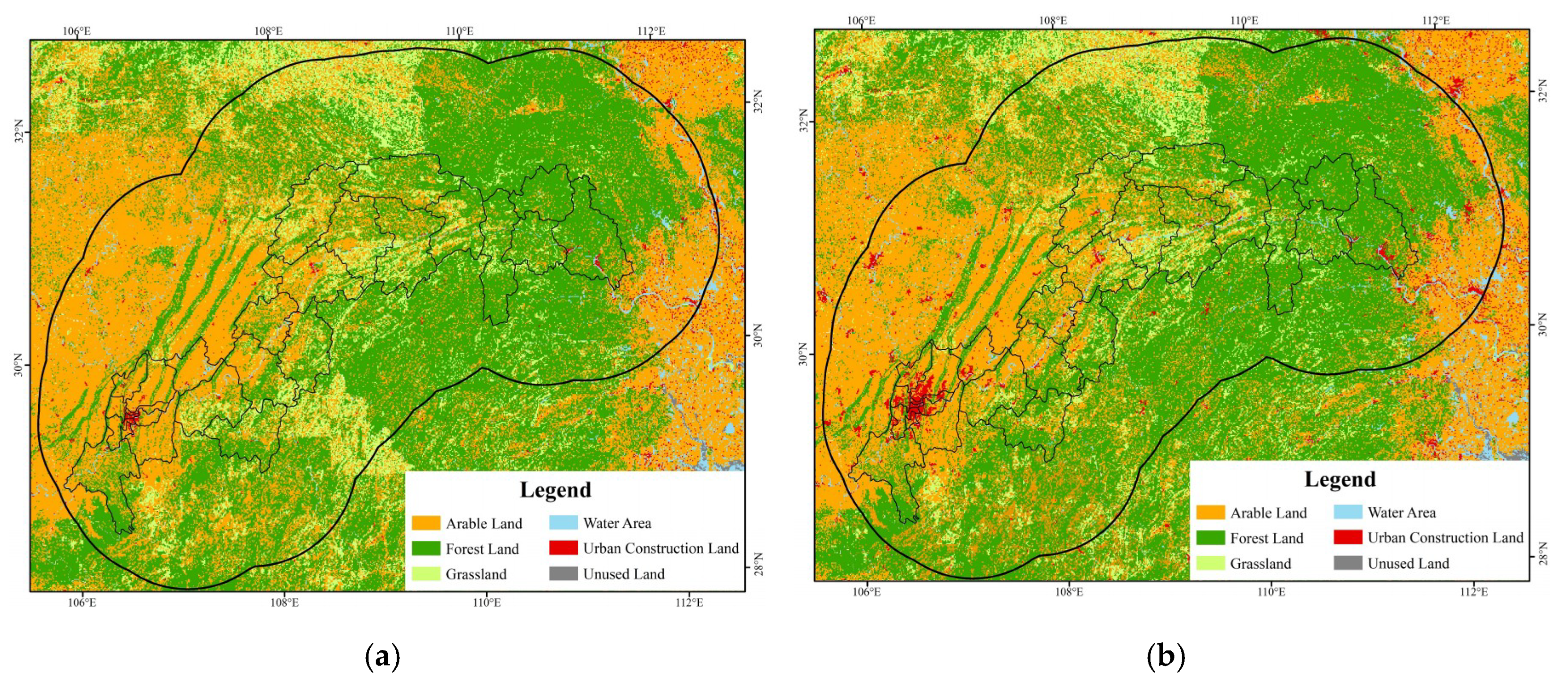
2.1. Study Area
2.2. Data
2.2.1. NDVI and Land Use/Land Cover Data
2.2.2. Meteorological Data
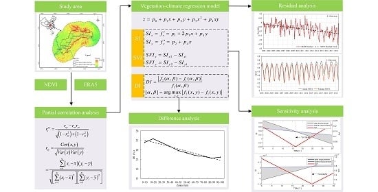
2.3. Methods
2.3.1. Partial Correlation Coefficient Method
2.3.2. Grid Point Analysis
2.3.3. Establish Vegetation–Climate Regression Model
2.3.4. Residual Analysis
2.3.5. Mann–Kendall Test
3. Results
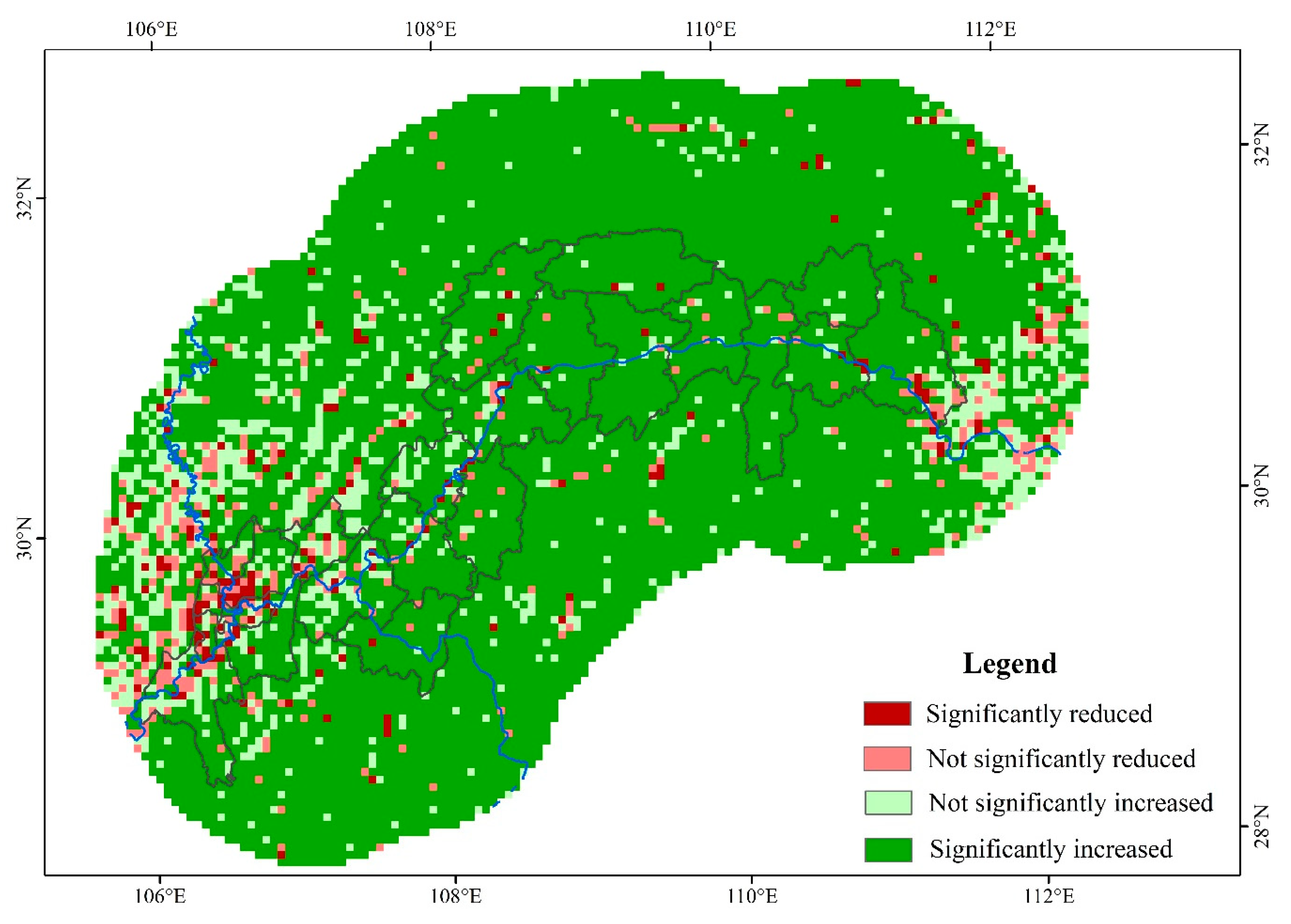
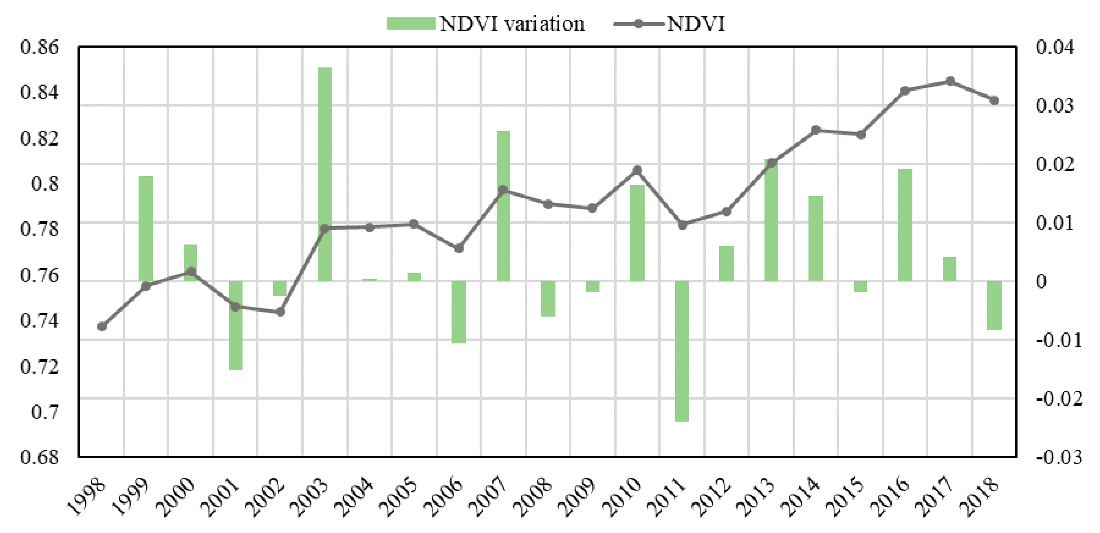
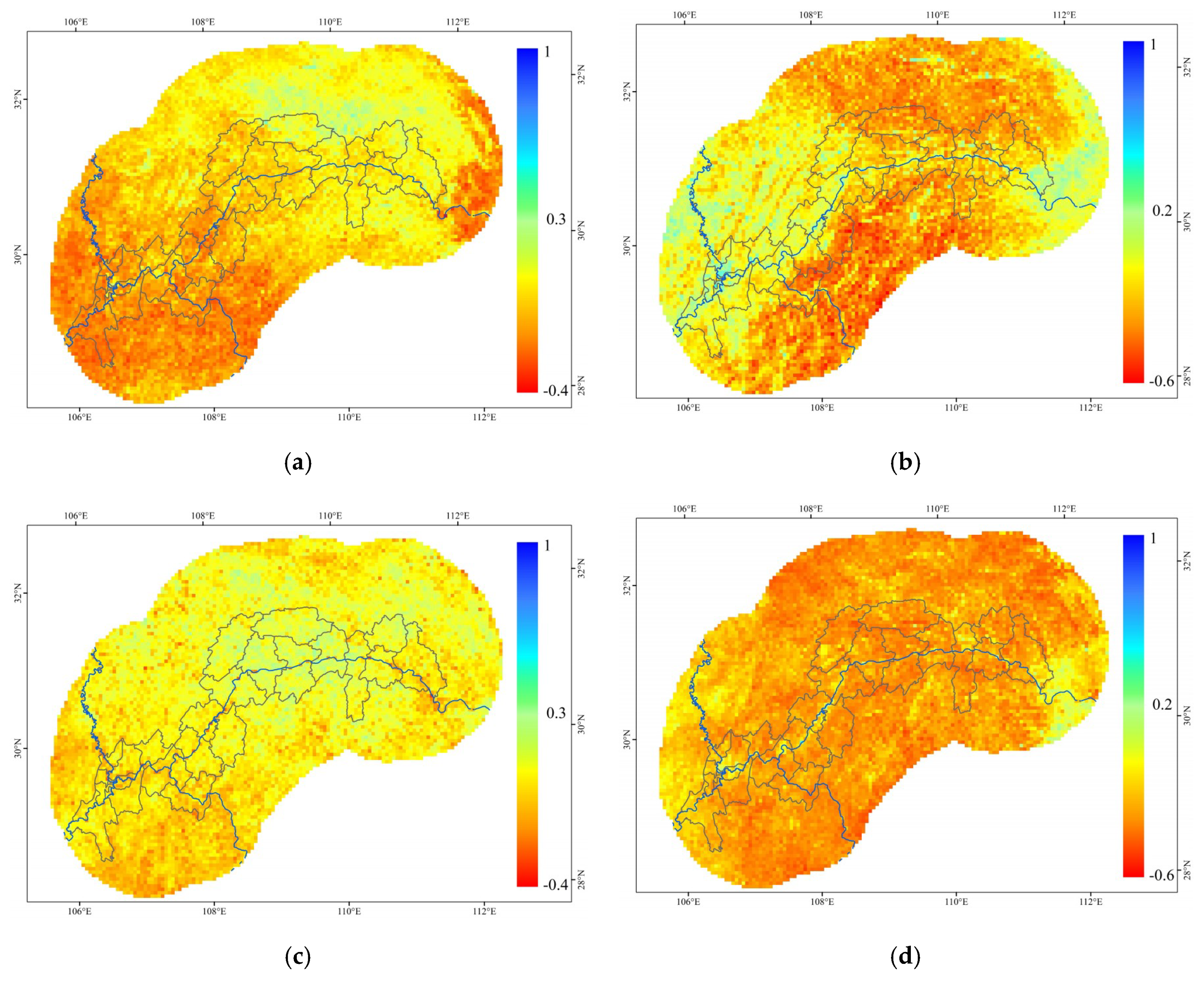
3.1. Vegetation Evolution Pattern around the Reservoir
3.2. Screening the Drivers of Vegetation Change
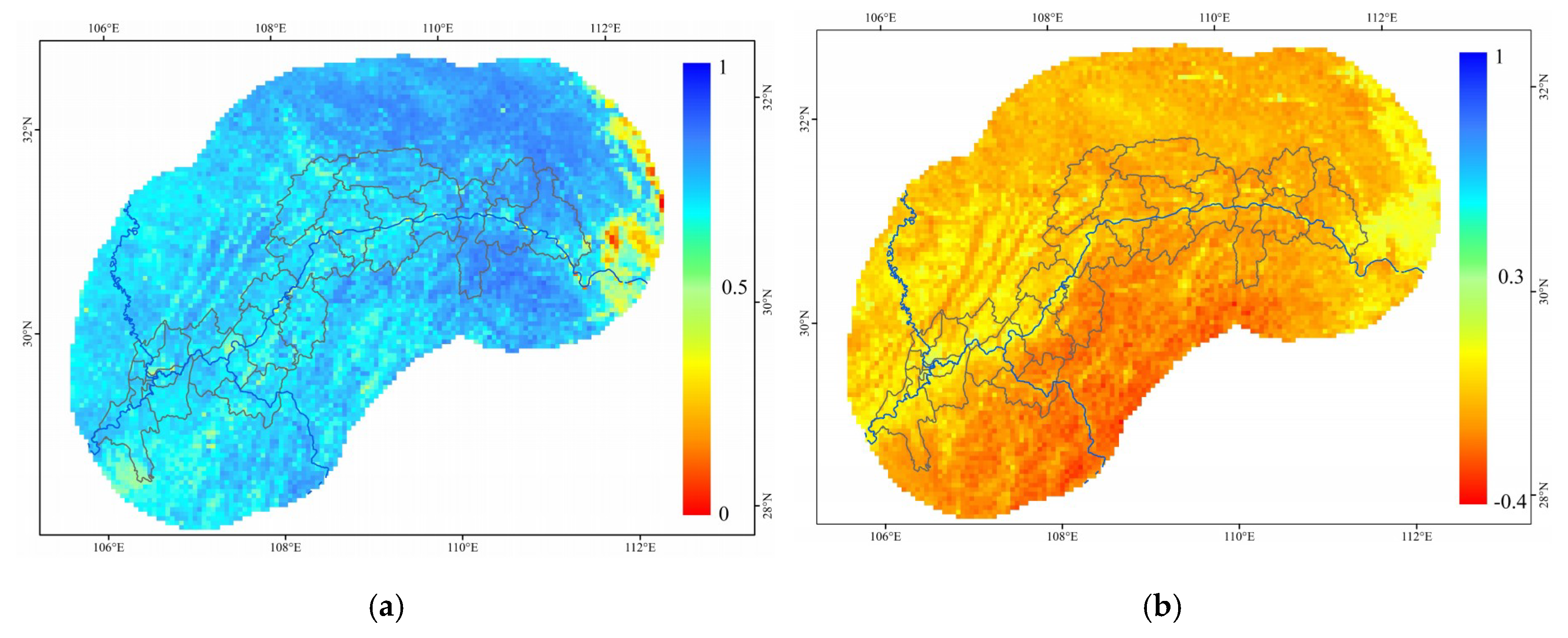
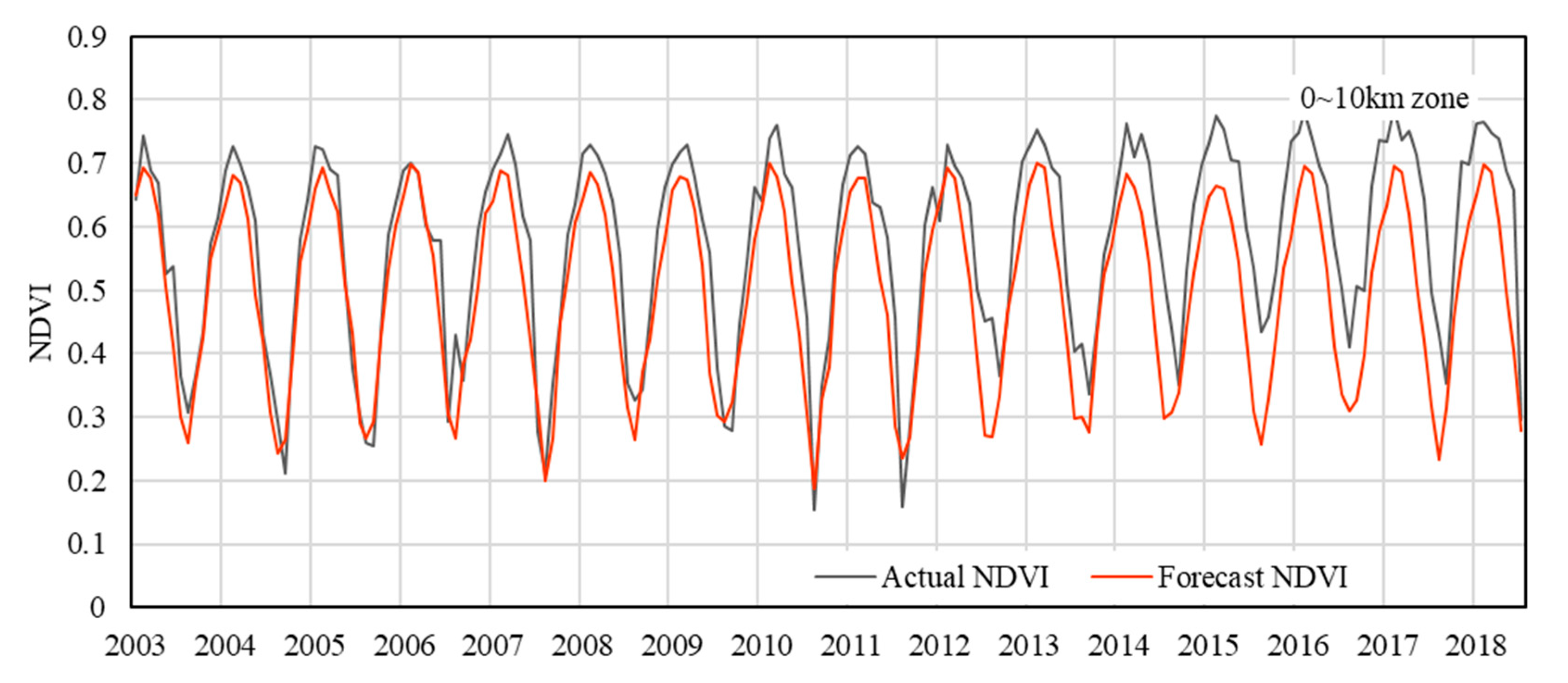
3.3. Vegetation–Climate Regression Model
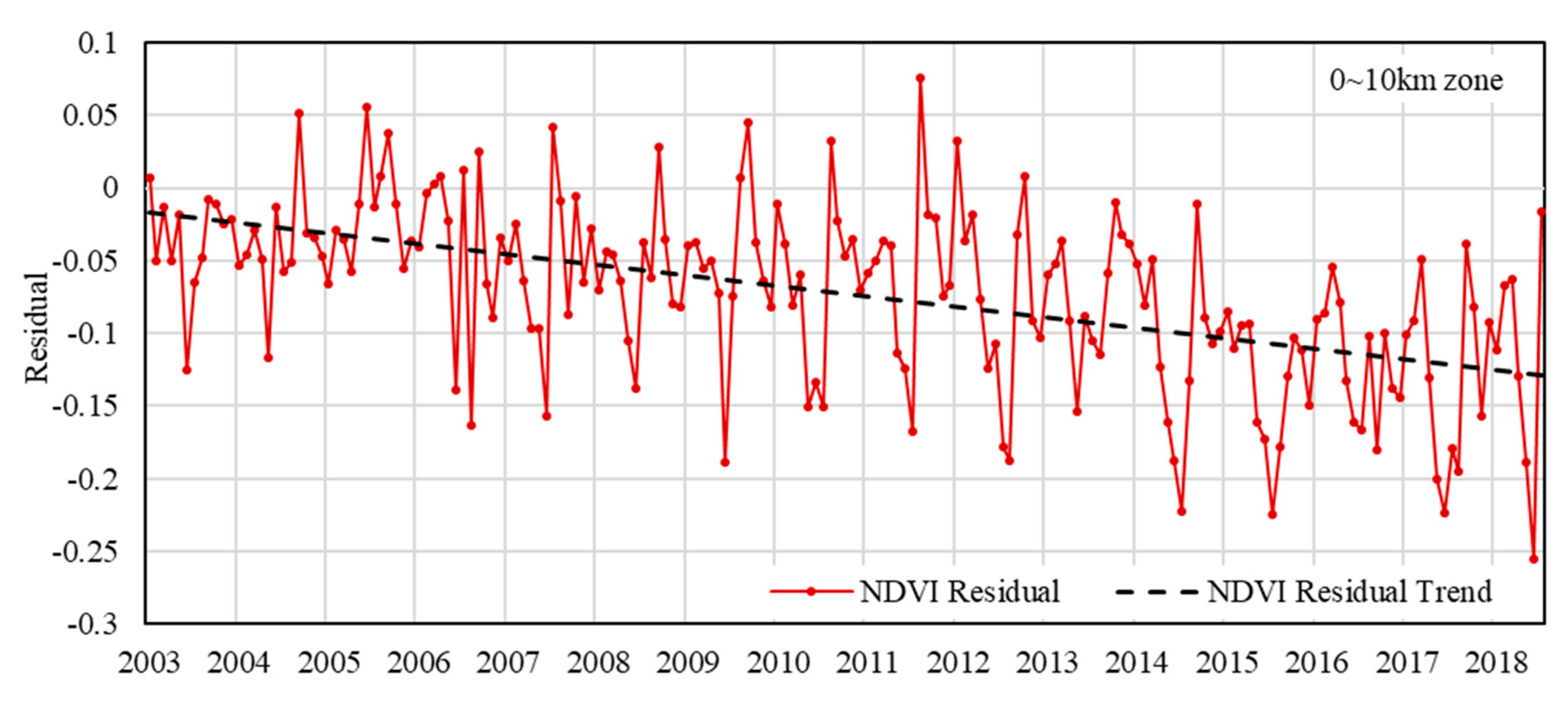
3.4. Residual Analysis
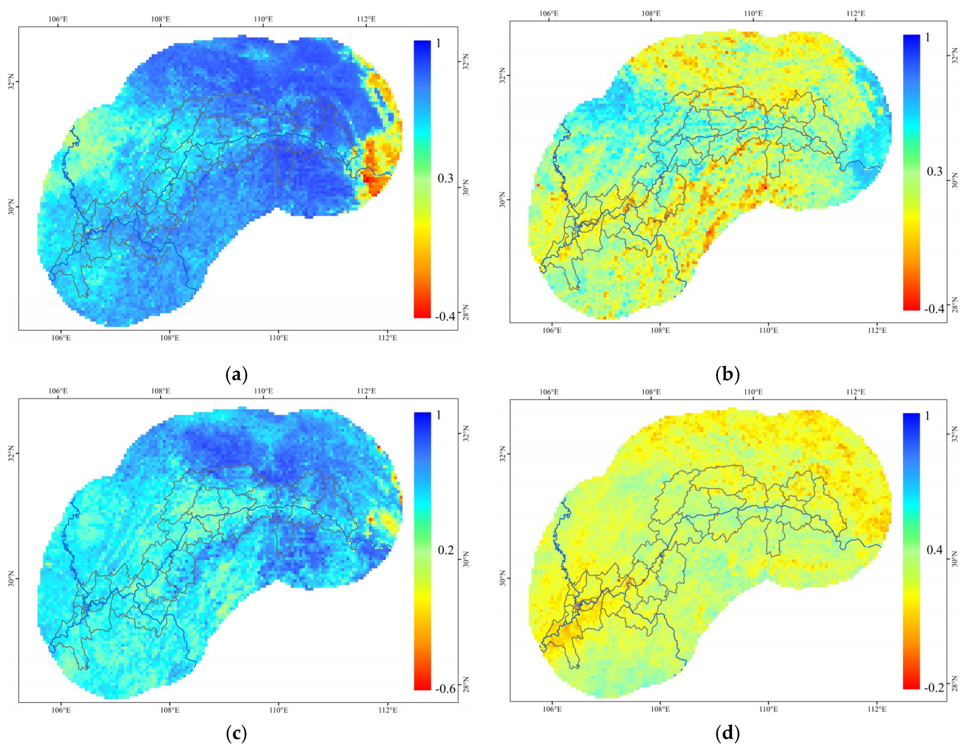
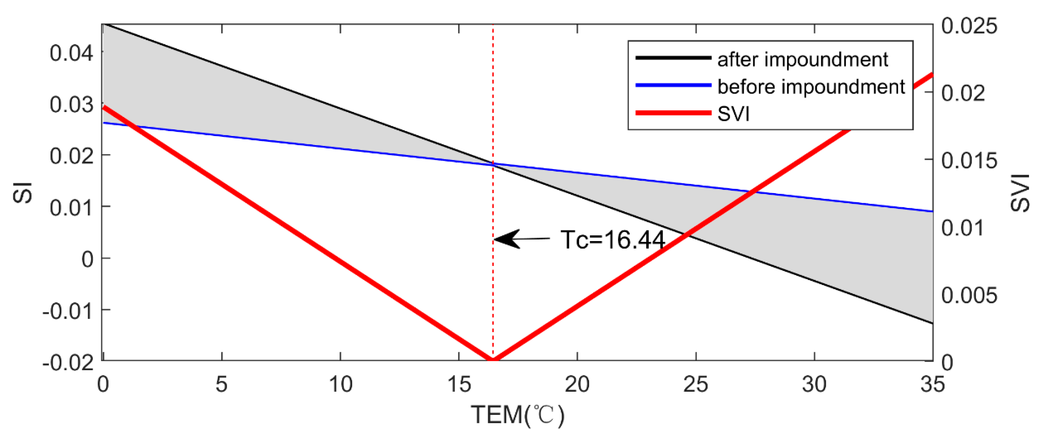
3.5. Sensitivity Analysis
3.6. Difference Analysis
4. Discussion
5. Conclusions
Author Contributions
Funding
Acknowledgments
Conflicts of Interest
References
- Sun, W.; Song, X.; Mu, X.; Gao, P.; Wang, F.; Zhao, G. Spatiotemporal vegetation cover variations associated with climate change and ecological restoration in the Loess Plateau. Agric. For. Meteorol. 2015, 209–210, 87–99. [Google Scholar] [CrossRef]
- Jia, K.; Liang, S.; Zhang, L.; Wei, X.; Yao, Y.; Xie, X. Forest cover classification using Landsat ETM+ data and time series MODIS NDVI data. Int. J. Appl. Earth Obs. Geoinf. 2014, 33, 32–38. [Google Scholar] [CrossRef]
- Bégué, A.; Vintrou, E.; Ruelland, D.; Claden, M.; Dessay, N. Can a 25-year trend in Soudano-Sahelian vegetation dynamics be interpreted in terms of land use change? A remote sensing approach. Glob. Environ. Chang. 2011, 21, 413–420. [Google Scholar] [CrossRef]
- Wang, Q.; Zhang, Q.; Zhou, W. Grassland coverage changes and analysis of the driving forces in Maqu County. Phys. Procedia 2012, 33, 1292–1297. [Google Scholar] [CrossRef]
- De Jong, R.; de Bruin, S.; de Wit, A.; Schaepman, M.E.; Dent, D.L. Analysis of monotonic greening and browning trends from global NDVI time-series. Remote Sens. Environ. 2011, 115, 692–702. [Google Scholar] [CrossRef]
- Chen, B.; Xu, G.; Coops, N.C.; Ciais, P.; Innes, J.L.; Wang, G.; Myneni, R.B.; Wang, T.; Krzyzanowski, J.; Li, Q.; et al. Changes in vegetation photosynthetic activity trends across the Asia-Pacific region over the last three decades. Remote Sens. Environ. 2014, 144, 28–41. [Google Scholar] [CrossRef]
- Krishnaswamy, J.; John, R.; Joseph, S. Consistent response of vegetation dynamics to recent climate change in tropical mountain regions. Glob. Chang. Biol. 2014, 20, 203–215. [Google Scholar] [CrossRef]
- Tousignant, M.Ê.; Pellerin, S.; Brisson, J. The relative impact of human disturbances on the vegetation of a large wetland complex. Wetlands 2010, 30, 333–344. [Google Scholar] [CrossRef]
- Root, T.L.; Price, J.T.; Hall, K.R.; Schneider, S.H.; Rosenzweig, C.; Pounds, J.A. Fingerprints of global warming on wild animals and plants. Nature 2003, 421, 57–60. [Google Scholar] [CrossRef]
- Piao, S.; Nan, H.; Huntingford, C.; Ciais, P.; Friedlingstein, P.; Sitch, S.; Peng, S.; Ahlström, A.; Canadell, J.G.; Cong, N.; et al. Evidence for a weakening relationship between interannual temperature variability and northern vegetation activity. Nat. Commun. 2014, 5, 6018. [Google Scholar] [CrossRef]
- Liu, Y.Y.; van Dijk, A.I.J.M.; McCabe, M.F.; Evans, J.P.; de Jeu, R.A.M. Global vegetation biomass change (1988–2008) and attribution to environmental and human drivers. Glob. Ecol. Biogeogr. 2013, 22, 692–705. [Google Scholar] [CrossRef]
- Strengers, B.J.; Müller, C.; Schaeffer, M.; Haarsma, R.J.; Severijns, C.; Gerten, D.; Schaphoff, S.; Van Den Houdt, R.; Oostenrijk, R. Assessing 20th century climate-vegetation feedbacks of land-use change and natural vegetation dynamics in a fully coupled vegetation-climate model. Int. J. Climatol. 2010, 30, 2055–2065. [Google Scholar] [CrossRef]
- Xu, G.; Zhang, H.; Chen, B.; Zhang, H.; Innes, J.L.; Wang, G.; Yan, J.; Zheng, Y.; Zhu, Z.; Myneni, R.B. Changes in vegetation growth dynamics and relations with climate over China’s landmass from 1982 to 2011. Remote Sens. 2014, 6, 3263–3283. [Google Scholar] [CrossRef]
- Huang, K.; Zhang, Y.; Zhu, J.; Liu, Y.; Zu, J.; Zhang, J. The influences of climate change and human activities on vegetation dynamics in the Qinghai-Tibet plateau. Remote Sens. 2016, 8, 876. [Google Scholar] [CrossRef]
- Horion, S.; Cornet, Y.; Erpicum, M.; Tychon, B. Studying interactions between climate variability and vegetation dynamic using a phenology based approach. Int. J. Appl. Earth Obs. Geoinf. 2012, 20, 20–32. [Google Scholar] [CrossRef]
- Zhao, X.; Tan, K.; Zhao, S.; Fang, J. Changing climate affects vegetation growth in the arid region of the northwestern China. J. Arid Environ. 2011, 75, 946–952. [Google Scholar] [CrossRef]
- Xin, Z.B.; Xu, J.X.; Zheng, W. Spatiotemporal variations of vegetation cover on the Chinese Loess Plateau (1981–2006): Impacts of climate changes and human activities. Sci. China Ser. D Earth Sci. 2008, 51, 67–78. [Google Scholar] [CrossRef]
- Xie, B.; Jia, X.; Qin, Z.; Shen, J.; Chang, Q. Vegetation dynamics and climate change on the Loess Plateau, China: 1982–2011. Reg. Environ. Chang. 2016, 16, 1583–1594. [Google Scholar] [CrossRef]
- Xu, X.; Chen, H.; Levy, J.K. Spatiotemporal vegetation cover variations in the Qinghai-Tibet Plateau under global climate change. Chin. Sci. Bull. 2008, 53, 915–922. [Google Scholar] [CrossRef]
- Kong, D.; Zhang, Q.; Singh, V.P.; Shi, P. Seasonal vegetation response to climate change in the Northern Hemisphere (1982–2013). Glob. Planet. Chang. 2017, 148, 1–8. [Google Scholar] [CrossRef]
- Piao, S.; Mohammat, A.; Fang, J.; Cai, Q.; Feng, J. NDVI-based increase in growth of temperate grasslands and its responses to climate changes in China. Glob. Environ. Chang. 2006, 16, 340–348. [Google Scholar] [CrossRef]
- Mohammat, A.; Wang, X.; Xu, X.; Peng, L.; Yang, Y.; Zhang, X.; Myneni, R.B.; Piao, S. Drought and spring cooling induced recent decrease in vegetation growth in Inner Asia. Agric. For. Meteorol. 2013, 178–179, 21–30. [Google Scholar] [CrossRef]
- Xu, H.J.; Wang, X.P.; Yang, T.B. Trend shifts in satellite-derived vegetation growth in Central Eurasia, 1982–2013. Sci. Total Environ. 2017, 579, 1658–1674. [Google Scholar] [CrossRef] [PubMed]
- Notaro, M.; Chen, G.; Yu, Y.; Wang, F.; Tawfik, A. Regional climate modeling of vegetation feedbacks on the Asian-Australian monsoon systems. J. Clim. 2017, 30, 1553–1582. [Google Scholar] [CrossRef]
- Johannsen, F.; Ermida, S.; Martins, J.P.A.; Trigo, I.F.; Nogueira, M.; Dutra, E. Cold bias of ERA5 summertime daily maximum land surface temperature over Iberian Peninsula. Remote Sens. 2019, 11, 2570. [Google Scholar] [CrossRef]
- Nogueira, M.; Albergel, C.; Boussetta, S.; Johannsen, F.; Trigo, I.; Ermida, S.; Martins, J.; Dutra, E. Role of vegetation in representing land surface temperature in the CHTESSEL (CY45R1) and SURFEX-ISBA (v8.1) land surface models: A case study over Iberia. Geosci. Model. Dev. Discuss. 2020, 1–29. [Google Scholar] [CrossRef]
- Zhang, Y.; Zhang, C.; Wang, Z.; Chen, Y.; Gang, C.; An, R.; Li, J. Vegetation dynamics and its driving forces from climate change and human activities in the Three-River Source Region, China from 1982 to 2012. Sci. Total Environ. 2016, 563–564, 210–220. [Google Scholar] [CrossRef]
- Hua, W.; Chen, H.; Zhou, L.; Xie, Z.; Qin, M.; Li, X.; Ma, H.; Huang, Q.; Sun, S. Observational quantification of climatic and human influences on vegetation greening in China. Remote Sens. 2017, 9, 425. [Google Scholar] [CrossRef]
- Brandt, M.; Rasmussen, K.; Peñuelas, J.; Tian, F.; Schurgers, G.; Verger, A.; Mertz, O.; Palmer, J.R.B.; Fensholt, R. Human population growth offsets climate-driven increase in woody vegetation in sub-Saharan Africa. Nat. Ecol. Evol. 2017, 1, 0081. [Google Scholar] [CrossRef]
- Li, S.; Yan, J.; Liu, X.; Wan, J. Response of vegetation restoration to climate change and human activities in Shaanxi-Gansu-Ningxia Region. J. Geogr. Sci. 2013, 23, 98–112. [Google Scholar] [CrossRef]
- Li, S.; Yang, S.; Liu, X.; Liu, Y.; Shi, M. NDVI-based analysis on the influence of climate change and human activities on vegetation restoration in the shaanxi-gansu-ningxia region, central China. Remote Sens. 2015, 7, 11163–11182. [Google Scholar] [CrossRef]
- Wang, H.; Liu, G.; Li, Z.; Ye, X.; Fu, B.; Lv, Y. Impacts of Drought and Human Activity on Vegetation Growth in the Grain for Green Program Region, China. Chin. Geogr. Sci. 2018, 28, 470–481. [Google Scholar] [CrossRef]
- Zhang, J.; Zhengjun, L.; Xiaoxia, S. Changing landscape in the Three Gorges Reservoir Area of Yangtze River from 1977 to 2005: Land use/land cover, vegetation cover changes estimated using multi-source satellite data. Int. J. Appl. Earth Obs. Geoinf. 2009, 11, 403–412. [Google Scholar] [CrossRef]
- Evans, J.; Geerken, R. Discrimination between climate and human-induced dryland degradation. J. Arid Environ. 2004, 57, 535–554. [Google Scholar] [CrossRef]
- Herrmann, S.M.; Anyamba, A.; Tucker, C.J. Recent trends in vegetation dynamics in the African Sahel and their relationship to climate. Glob. Environ. Chang. 2005, 15, 394–404. [Google Scholar] [CrossRef]
- Wessels, K.J.; van den Bergh, F.; Scholes, R.J. Limits to detectability of land degradation by trend analysis of vegetation index data. Remote Sens. Environ. 2012, 125, 10–22. [Google Scholar] [CrossRef]
- Jiang, L.; Jiapaer, G.; Bao, A.; Guo, H.; Ndayisaba, F. Vegetation dynamics and responses to climate change and human activities in Central Asia. Sci. Total Environ. 2017, 599–600, 967–980. [Google Scholar] [CrossRef]
- Sun, Y.; Yang, Y.; Zhang, L.; Wang, Z. The relative roles of climate variations and human activities in vegetation change in North China. Phys. Chem. Earth 2015, 87–88, 67–78. [Google Scholar] [CrossRef]
- Wang, J.; Wang, K.; Zhang, M.; Zhang, C. Impacts of climate change and human activities on vegetation cover in hilly southern China. Ecol. Eng. 2015, 81, 451–461. [Google Scholar] [CrossRef]
- Wen, Z.; Wu, S.; Chen, J.; Lü, M. NDVI indicated long-term interannual changes in vegetation activities and their responses to climatic and anthropogenic factors in the Three Gorges Reservoir Region, China. Sci. Total Environ. 2017, 574, 947–959. [Google Scholar] [CrossRef]
- Caesagtgp, S. Staged Assessment Report of the Three Gorges Project (Comprehensive Volume); Chinese Water Power Press: Beijing, China, 2010. [Google Scholar]
- Wu, J.; Huang, J.; Han, X.; Gao, X.; He, F.; Jiang, M.; Jiang, Z.; Primack, R.B.; Shen, Z. The Three Gorges Dam: An ecological perspective. Front. Ecol. Environ. 2004, 2, 241–248. [Google Scholar] [CrossRef]
- Kerr, J.T.; Ostrovsky, M. From space to species: Ecological applications for remote sensing. Trends Ecol. Evol. 2003, 18, 299–305. [Google Scholar] [CrossRef]
- Turner, W.; Spector, S.; Gardiner, N.; Fladeland, M.; Sterling, E.; Steininger, M. Remote sensing for biodiversity science and conservation. Trends Ecol. Evol. 2003, 18, 306–314. [Google Scholar] [CrossRef]
- Yao, B.; Teng, S.; Lai, R.; Xu, X.; Yin, Y.; Shi, C.; Liu, C. Can atmospheric reanalyses (CRA and ERA5) represent cloud spatiotemporal characteristics? Atmos. Res. 2020, 244, 105091. [Google Scholar] [CrossRef]
- Lyu, F.; Tang, G.; Behrangi, A.; Wang, T.; Tan, X.; Ma, Z.; Xiong, W. Precipitation Merging Based on the Triple Collocation Method Across Mainland China. IEEE Trans. Geosci. Remote Sens. 2020, 1–16. [Google Scholar] [CrossRef]
- Yang, J.; Gong, P.; Fu, R.; Zhang, M.; Chen, J.; Liang, S.; Xu, B.; Shi, J.; Dickinson, R. The role of satellite remote sensing in climate change studies. Nat. Clim. Chang. 2013, 3, 875–883. [Google Scholar] [CrossRef]
- Wang, X.; Yang, F.; Gao, X.; Wang, W.; Zha, X. Evaluation of Forest Damaged Area and Severity Caused by Ice-snow Frozen Disasters over Southern China with Remote Sensing. Chin. Geogr. Sci. 2019, 29, 405–416. [Google Scholar] [CrossRef]
- Di, L.; Yu, E.; Shrestha, R.; Lin, L. DVDI: A new remotely sensed index for measuring vegetation damage caused by natural disasters. Int. Geosci. Remote Sens. Symp. 2018, 2018, 9067–9069. [Google Scholar] [CrossRef]
- Klisch, A.; Atzberger, C. Operational drought monitoring in Kenya using MODIS NDVI time series. Remote Sens. 2016, 8, 267. [Google Scholar] [CrossRef]
- Beck, P.S.A.; Atzberger, C.; Høgda, K.A.; Johansen, B.; Skidmore, A.K. Improved monitoring of vegetation dynamics at very high latitudes: A new method using MODIS NDVI. Remote Sens. Environ. 2006, 100, 321–334. [Google Scholar] [CrossRef]
- Neigh, C.S.R.; Tucker, C.J.; Townshend, J.R.G. North American vegetation dynamics observed with multi-resolution satellite data. Remote Sens. Environ. 2008, 112, 1749–1772. [Google Scholar] [CrossRef]
- Pettorelli, N.; Vik, J.O.; Mysterud, A.; Gaillard, J.M.; Tucker, C.J.; Stenseth, N.C. Using the satellite-derived NDVI to assess ecological responses to environmental change. Trends Ecol. Evol. 2005, 20, 503–510. [Google Scholar] [CrossRef] [PubMed]
- Running, S.W. Estimating Terrestrial Primary Productivity by Combining Remote Sensing and Ecosystem Simulation. Remote Sens. Biosph. Funct. 1990, 65–86. [Google Scholar] [CrossRef]
- Myneni, R.B.; Hall, F.G.; Sellers, P.J.; Marshak, A.L. Interpretation of spectral vegetation indexes. IEEE Trans. Geosci. Remote Sens. 1995, 33, 481–486. [Google Scholar] [CrossRef]
- Data Center for Resources and Environmental Sciences, Chinese Academy of Sciences. NDVI Spatial Distribution Dataset in China. Available online: http://www.resdc.cn (accessed on 11 February 2020).
- Data Center for Resources and Environmental Sciences, Chinese Academy of Sciences. Land Use/Land Cover Remote Sensing Monitoring Dataset in China. Available online: http://www.resdc.cn (accessed on 5 August 2020).
- Liu, J.; Zhang, Z.; Xu, X.; Kuang, W.; Zhou, W.; Zhang, S.; Li, R.; Yan, C.; Yu, D.; Wu, S.; et al. Spatial patterns and driving forces of land use change in China during the early 21st century. J. Geogr. Sci. 2010, 20, 483–494. [Google Scholar] [CrossRef]
- Climate Data Store. Available online: https://cds.climate.copernicus.eu/ (accessed on 16 February 2019).
- Albergel, C.; Dutra, E.; Munier, S.; Calvet, J.C.; Munoz-Sabater, J.; De Rosnay, P.; Balsamo, G. ERA-5 and ERA-Interim driven ISBA land surface model simulations: Which one performs better? Hydrol. Earth Syst. Sci. 2018, 22, 3515–3532. [Google Scholar] [CrossRef]
- Nogueira, M. Inter-comparison of ERA-5, ERA-interim and GPCP rainfall over the last 40 years: Process-based analysis of systematic and random differences. J. Hydrol. 2020, 583, 124632. [Google Scholar] [CrossRef]
- Tarek, M.; Brissette, F.; Arsenault, R. Evaluation of the ERA5 reanalysis as a potential reference dataset for hydrological modeling over North-America. Hydrol. Earth Syst. Sci. Discuss. 2020, 24, 2527–2544. [Google Scholar] [CrossRef]
- Tang, G.; Clark, M.P.; Papalexiou, S.M.; Ma, Z.; Hong, Y. Have satellite precipitation products improved over last two decades? A comprehensive comparison of GPM IMERG with nine satellite and reanalysis datasets. Remote Sens. Environ. 2020, 240, 111697. [Google Scholar] [CrossRef]
- Yang, H.; He, C.; Wang, Z.; Shao, W. Reliability Analysis of European ERA5 Water Vapor Content Based on Ground-based GPS in China. Atlantis Press 2019, 89, 44–49. [Google Scholar] [CrossRef][Green Version]
- Zhang, W.; Zhang, H.; Liang, H.; Lou, Y.; Cai, Y.; Cao, Y.; Zhou, Y.; Liu, W. On the suitability of ERA5 in hourly GPS precipitable water vapor retrieval over China. J. Geod. 2019, 93, 1897–1909. [Google Scholar] [CrossRef]
- Mann, H.B. Nonparametric tests against trend. Econometrica 1945, 13, 245. [Google Scholar] [CrossRef]
- Kendall, M.G. Rank correlation methods. Biometrika 1957, 44, 298. [Google Scholar] [CrossRef]
- Xiang, F.; Wang, L.; Yao, R.; Niu, Z. The characteristics of climate change and response of vegetation in three gorges reservoir area. Earth Sci. 2018, 43, 42–52. (In Chinese) [Google Scholar] [CrossRef]
- Zhang, L.; Shen, J.; Liu, X.; Zhu, W. Vegetation changes in the three gorges reservoir area from 2001 to 2016 and the analysis of its climate driving factors. Geogr. Geo Inf. Sci. 2019, 35, 38–46. (In Chinese) [Google Scholar] [CrossRef]
- Clifford, M.J.; Royer, P.D.; Cobb, N.S.; Breshears, D.D.; Ford, P.L. Precipitation thresholds and drought-induced tree die-off: Insights from patterns of Pinus edulis mortality along an environmental stress gradient. New Phytol. 2013, 200, 413–421. [Google Scholar] [CrossRef]
- Zhang, K.; Kimball, J.S.; Nemani, R.R.; Running, S.W.; Hong, Y.; Gourley, J.J.; Yu, Z. Vegetation Greening and Climate Change Promote Multidecadal Rises of Global Land Evapotranspiration. Sci. Rep. 2015, 5, 15956. [Google Scholar] [CrossRef]
- Gourdji, S.M.; Sibley, A.M.; Lobell, D.B. Global crop exposure to critical high temperatures in the reproductive period: Historical trends and future projections. Environ. Res. Lett. 2013, 8, 024041. [Google Scholar] [CrossRef]
- Jiao, K.; Gao, J.; Wu, S.; Hou, W. Research progress on the response processes of vegetation activity to climate change. Acta Ecol. Sin. 2018, 38, 2229–2238. (In Chinese) [Google Scholar] [CrossRef]


| Spring | Summer | Autumn | Winter | Total Series | |
|---|---|---|---|---|---|
| Average rN-t | 0.654 | 0.268 | 0.532 | 0.295 | 0.718 |
| Percentage of |rN-t| ≥ 0.4 | 92.086% | 23.699% | 83.231% | 10.075% | 98.47% |
| Average rN-p | −0.037 | −0.163 | 0.057 | −0.282 | −0.090 |
| Percentage of |rN-p| ≥ 0.4 | 0.034% | 9.874% | 0 | 9.123% | 0 |
| Zones (km) | Before Impoundment | After Impoundment | ||||||||
|---|---|---|---|---|---|---|---|---|---|---|
| p0 | p1 | p2 (10−5) | p3 (10−5) | p4 (10−6) | p0 | p1 | p2 (10−3) | p3 (10−4) | p4 (10−5) | |
| 0–10 | 0.160 | 0.026 | −1.176 | −25.1 | 4.764 | 0.212 | 0.040 | −1.136 | −8.252 | 5.065 |
| 10–20 | 0.179 | 0.025 | 1.871 | −20.29 | 1.527 | 0.239 | 0.041 | −1.288 | −8.385 | 5.578 |
| 20–30 | 0.209 | 0.023 | −2.125 | −10.44 | 1.035 | 0.259 | 0.039 | −1.278 | −7.8 | 5.457 |
| 30–40 | 0.217 | 0.022 | −2.628 | −6.946 | −0.329 | 0.264 | 0.038 | −1.231 | −7.227 | 5.175 |
| 40–50 | 0.218 | 0.022 | −12.73 | −7.649 | 3.68 | 0.255 | 0.038 | −1.298 | −7.168 | 5.442 |
| 50–60 | 0.220 | 0.023 | −14.48 | −8.769 | 4.098 | 0.258 | 0.037 | −1.261 | −6.909 | 5.274 |
| 60–70 | 0.228 | 0.022 | −18.55 | −7.109 | 5.334 | 0.261 | 0.036 | −1.21 | −6.593 | 5.072 |
| 70–80 | 0.223 | 0.021 | −18.27 | −4.098 | 5.491 | 0.255 | 0.035 | −1.15 | −6.115 | 4.889 |
| 80–90 | 0.236 | 0.021 | −18.96 | −3.693 | 5.806 | 0.266 | 0.035 | −1.087 | −5.861 | 4.53 |
| 90–100 | 0.225 | 0.021 | −14.87 | −3.966 | 4.28 | 0.256 | 0.035 | −1.075 | −5.848 | 4.444 |
| Zones | Before Impoundment | After Impoundment | ||||
|---|---|---|---|---|---|---|
| SSE | R2 | p | SSE | R2 | p | |
| 0–10 | 0.1171 | 0.913 | 1.56 × 10⁻²⁹ * | 0.6394 | 0.854 | 7.39 × 10−75 * |
| 10–20 | 0.1281 | 0.908 | 7.82 × 10⁻²⁹ * | 0.6687 | 0.852 | 3.12 × 10−74 * |
| 20–30 | 0.1357 | 0.902 | 4.65 × 10⁻²⁸ * | 0.6588 | 0.853 | 1.81 × 10−74 * |
| 30–40 | 0.1508 | 0.893 | 5.70 × 10⁻²⁷ * | 0.6262 | 0.861 | 8.80 × 10−77 * |
| 40–50 | 0.1443 | 0.900 | 9.82 × 10⁻²⁸ * | 0.5891 | 0.873 | 1.78 × 10−80 * |
| 50–60 | 0.1436 | 0.899 | 1.17 × 10⁻²⁷ * | 0.5749 | 0.876 | 2.69 × 10−81 * |
| 60–70 | 0.1409 | 0.900 | 9.73 × 10⁻²⁸ * | 0.567 | 0.878 | 6.84 × 10−82 * |
| 70–80 | 0.1304 | 0.909 | 5.84 × 10⁻²⁹ * | 0.5479 | 0.884 | 6.77 × 10−84 * |
| 80–90 | 0.1292 | 0.906 | 1.43 × 10⁻²⁸ * | 0.5485 | 0.880 | 1.26 × 10−82 * |
| 90–100 | 0.1263 | 0.910 | 4.05 × 10⁻²⁹ * | 0.5258 | 0.887 | 7.19 × 10−85 * |
| Zones | k (10−4) | p |
|---|---|---|
| 0–10 km | −6.030 | 7.51 × 10⁻¹⁵ * |
| 10–20 km | −6.020 | 2.09 × 10⁻¹⁴ * |
| 20–30 km | −6.015 | 8.28 × 10⁻¹⁴ * |
| 30–40 km | −6.006 | 1.83 × 10⁻¹³ * |
| 40–50 km | −6.004 | 2.73 × 10⁻¹³ * |
| 50–60 km | −5.999 | 2.13 × 10⁻¹³ * |
| 60–70 km | −5.997 | 2.62 × 10⁻¹³ * |
| 70–80 km | −6.006 | 5.72 × 10⁻¹³ * |
| 80–90 km | −6.005 | 3.59 × 10⁻¹³ * |
| 90–100 km | −6.007 | 4.06 × 10⁻¹³ * |
| Zones | Before Impoundment | After Impoundment | Tc (°C) | ||||||
|---|---|---|---|---|---|---|---|---|---|
| p1 | 2p3 (10−5) | p4 (10−6) | p1 | 2p3 (10−4) | p4 (10−5) | Pre = 100 mm | Pre = 200 mm | Pre = 300 mm | |
| 0–10 | 0.026 | −50.2 | 4.764 | 0.040 | −16.50 | 5.065 | 16.44 | 20.43 | 24.43 |
| 10–20 | 0.025 | −40.58 | 1.527 | 0.041 | −16.77 | 5.578 | 16.41 | 20.68 | 24.95 |
| 20–30 | 0.023 | −20.88 | 1.035 | 0.039 | −15.60 | 5.457 | 16.1 | 20.06 | 24.02 |
| 30–40 | 0.022 | −13.89 | −0.329 | 0.038 | −14.45 | 5.175 | 16.02 | 20.01 | 24 |
| 40–50 | 0.022 | −15.30 | 3.680 | 0.038 | −14.34 | 5.442 | 16.18 | 20.14 | 24.1 |
| 50–60 | 0.023 | −17.54 | 4.098 | 0.037 | −13.82 | 5.274 | 16.22 | 20.25 | 24.29 |
| 60–70 | 0.022 | −14.22 | 5.334 | 0.036 | −13.19 | 5.072 | 16.18 | 20.04 | 23.9 |
| 70–80 | 0.021 | −8.20 | 5.491 | 0.035 | −12.23 | 4.889 | 16.03 | 19.84 | 23.64 |
| 80–90 | 0.021 | −7.39 | 5.806 | 0.035 | −11.72 | 4.53 | 16.16 | 19.75 | 23.35 |
| 90–100 | 0.021 | −7.93 | 4.280 | 0.035 | −11.70 | 4.444 | 16.24 | 19.93 | 23.61 |
| Zones | Before Impoundment | After Impoundment | Tc (°C) | ||
|---|---|---|---|---|---|
| p2 (10−5) | p4 (10−6) | p2 (10−3) | p4 (10−5) | ||
| 0–10 | −1.176 | 4.764 | −1.136 | 5.065 | 24.29 |
| 10–20 | 1.871 | 1.527 | −1.288 | 5.578 | 23.91 |
| 20–30 | −2.125 | 1.035 | −1.278 | 5.457 | 23.29 |
| 30–40 | −2.628 | −0.329 | −1.231 | 5.175 | 22.95 |
| 40–50 | −12.73 | 3.680 | −1.298 | 5.442 | 22.88 |
| 50–60 | −14.48 | 4.098 | −1.261 | 5.274 | 22.75 |
| 60–70 | −18.55 | 5.334 | −1.210 | 5.072 | 22.36 |
| 70–80 | −18.27 | 5.491 | −1.150 | 4.889 | 22.06 |
| 80–90 | −18.96 | 5.806 | −1.087 | 4.530 | 22.47 |
| 90–100 | −14.87 | 4.280 | −1.075 | 4.444 | 22.82 |
© 2020 by the authors. Licensee MDPI, Basel, Switzerland. This article is an open access article distributed under the terms and conditions of the Creative Commons Attribution (CC BY) license (http://creativecommons.org/licenses/by/4.0/).
Share and Cite
Tian, M.; Zhou, J.; Jia, B.; Lou, S.; Wu, H. Impact of Three Gorges Reservoir Water Impoundment on Vegetation–Climate Response Relationship. Remote Sens. 2020, 12, 2860. https://doi.org/10.3390/rs12172860
Tian M, Zhou J, Jia B, Lou S, Wu H. Impact of Three Gorges Reservoir Water Impoundment on Vegetation–Climate Response Relationship. Remote Sensing. 2020; 12(17):2860. https://doi.org/10.3390/rs12172860
Chicago/Turabian StyleTian, Mengqi, Jianzhong Zhou, Benjun Jia, Sijing Lou, and Huiling Wu. 2020. "Impact of Three Gorges Reservoir Water Impoundment on Vegetation–Climate Response Relationship" Remote Sensing 12, no. 17: 2860. https://doi.org/10.3390/rs12172860
APA StyleTian, M., Zhou, J., Jia, B., Lou, S., & Wu, H. (2020). Impact of Three Gorges Reservoir Water Impoundment on Vegetation–Climate Response Relationship. Remote Sensing, 12(17), 2860. https://doi.org/10.3390/rs12172860