Artificial Neural Networks to Retrieve Land and Sea Skin Temperature from IASI

Abstract

Surface skin temperature (T_skin) derived from infrared remote sensors mounted on board satellites provides a continuous observation of Earth’s surface and allows the monitoring of global temperature change relevant to climate trends. In this study, we present a fast retrieval method for retrieving T_skin based on an artificial neural network (ANN) from a set of spectral channels selected from the Infrared Atmospheric Sounding Interferometer (IASI) using the information theory/entropy reduction technique. Our IASI T_skin product (i.e., T_ANN) is evaluated against T_skin from EUMETSAT Level 2 product, ECMWF Reanalysis (ERA5), SEVIRI observations, and ground in situ measurements. Good correlations between IASI T_ANN and the T_skin from other datasets are shown by their statistic data, such as a mean bias and standard deviation (i.e., [bias, STDE]) of [0.55, 1.86 °C], [0.19, 2.10 °C], [−1.5, 3.56 °C], from EUMETSAT IASI L-2 product, ERA5, and SEVIRI. When compared to ground station data, we found that all datasets did not achieve the needed accuracy at several months of the year, and better results were achieved at nighttime. Therefore, comparison with ground-based measurements should be done with care to achieve the ±2 °C accuracy needed, by choosing, for example, a validation site near the station location. On average, this accuracy is achieved, in particular at night, leading to the ability to construct a robust T_skin dataset suitable for T_skin long-term spatio-temporal variability and trend analysis.

1. Introduction

Land surface temperature, radiometric temperature, or as used hereafter, skin temperature, T_skin, depends on the energy fluxes between the surface and the atmosphere. It is an important factor for studying the Earth’s energy balance, convection at the surface, monitoring droughts, and in numerical weather prediction [1,2,3]. Although in situ observations play a major role in measuring relevant climate change indicators, local measurements are sparse and unevenly distributed. Global view observations are now routinely available from remote sensors on satellites, providing data from which climate variables such as T_skin can be derived using appropriate retrieval methods. The World Meteorological Organization (WMO) Global Climate Observing System (GCOS) program aims at identifying requirements for the global climate monitoring system. It recommends 54 key variables (https://gcos.wmo.int/en/essential-climate-variables/), called Essential Climate Variables (ECVs), as the atmospheric, land, and ocean components of this monitoring system. Near-surface temperature and skin temperature are both ECVs. In the thermal infrared spectral range, satellites do not measure the well-known thermodynamic near-surface air temperatures (T_2m); instead, they measure the skin temperature. It is called “skin” temperature since it corresponds to the radiation emitted from depths less than or equal to the penetration depth at a given wavelength [4], which can be as small as 10–20 micrometers at the ocean surface [5]. The relationship between T_skin and T_2m is complex: differences between T_skin and T_2m can reach several to ten or more degrees under cloud-free, low wind speed conditions, and is usually smaller under cloudy conditions or when solar insolation is low [6,7,8].

Satellite retrievals of skin temperatures are available from a variety of polar-orbiting and geostationary platforms carrying microwave and infrared sensors, such as the Spinning Enhanced Visible and Infrared Imager (SEVIRI) onboard the geostationary Meteosat Second Generation [9], the Advanced Very High Resolution Radiometer (AVHRR) sensors onboard the different NOAA polar orbiting platforms and more recently on the suite of Metop satellites [10], the Moderate Resolution Imaging Spectroradiometer (MODIS) on board of the Terra and Aqua satellites [11], the Atmospheric InfraRed Sounder (AIRS) [12] on board the Aqua satellite, and from the Infrared Atmospheric Sounding Interferometer (IASI) on board the three Metop satellites since 2006, 2012, and 2018 [13,14,15].

With a polar orbit, IASI on Metop revisits all points on the Earth’s surface twice a day at around 9:30 a.m. and 9:30 p.m. local time. IASI is designed for numerical weather prediction, climate research, and atmospheric composition monitoring [15,16,17]. It measures radiances in the thermal infrared spectral range between 645 and 2760 cm⁻¹, corresponding to 8461 spectral channels, every 0.25 cm⁻¹, with an instrument response function of 0.5 cm⁻¹ half-width after apodization. With more than 13 years of data that are now readily available, the instrument provides more than 1.2 million radiance spectra per day, with a footprint on the ground of 12 km diameter pixel (at nadir). IASI scenes are reduced by around one-third when clear sky filtering (<10% cloud coverage) is applied, a necessity for accessing information at the surface. IASI has been used for atmospheric composition sounding, allowing near-real-time mapping of chemical species and aerosols, contributing to air traffic safety, and improving the understanding of atmospheric transport processes [18,19,20].

The interest in exploiting highly spectrally resolved IASI data to study climate variability has been previously highlighted [21,22,23,24]; preliminary T_skin trends from Metop-A IASI measurements were presented at the SPIE conference [25]. Although the spectral signature of climate variability and T_skin anomalies have been studied for similar instruments [26,27], relatively little has been done to generate systematic climate-data records for surface and atmospheric parameters with IASI measurements. The instrument is relatively new (radiances are provided since July 2007) and the climate community is still not fully aware of its potential. It is also computationally demanding to systematically process the large amount of data generated by the instrument. However, since IASI is planned to fly for at least 18 years, with the three instruments built at the same time and flying in constellation, continuity and stability are insured, and the potential of constructing a long-term climate data record is becoming evident. In addition, it is worth noting that the long-term continuation of the program is also guaranteed, as the new generation of Infrared Atmospheric Sounding Interferometers (IASI-NG) [28,29] will be launched on three successive Metop—Second Generation satellites within the 2022–2040 timeframe.

IASI data are disseminated by EUMETSAT (EUropean organization for the exploitation of METeorological SATellites) [30]. It processes a T_skin product from the series of the Metop satellites for day-to-day meteorological applications. This T_skin product is derived from IASI upwelling radiances but also relies on two microwave instruments (Microwave Humidity Sounder, MHS, and The Advanced Microwave Sounding Unit-A, AMSU-A) on board Metop, particularly for cloudy scenes. Changes occurred with evolving versions of the processing algorithm [31,32], with the algorithm mostly stable after 2016. The Metop-A L1C (radiance spectra) record has been reprocessed back in time at EUMETSAT for the period 2007–2017, and is used in this work, and has been available since late 2019 [33]. L1C data after 2017 are not reprocessed because they are assumed to be up to date. The Level 2 series (T_skin, H₂O, cloud information, etc.) has not yet been reprocessed back in time, which complicates the construction of a homogeneous T_skin data record from IASI.

More generally, high volumes of data resulting from IASI present many challenges in data transmission, storage, and assimilation. One of the simplest methods for reducing the data volume is channel selection. The goal of this study is to present a fast and reliable method developed to retrieve T_skin from radiances using a limited set of radiances from the 2019 reprocessed IASI L1C data record in the thermal infrared in order to have a consistent and homogeneous product covering the whole IASI sounding period. The challenge is therefore to find the optimal set of channels from which skin temperature can be retrieved. In the following Section 2, we present an approach based on entropy reduction [34,35] from which we deduce a set of 100 channels, which are among the most sensitive channels to T_skin. This new IASI L1C dataset is then used to retrieve skin temperature from IASI’s cloud-free radiances using an artificial neural network (ANN). In Section 3 we validate the product and we conclude this paper with a discussion in Section 4 of the current challenges in the validation and comparison of different T_skin products.

2. Data and Methods

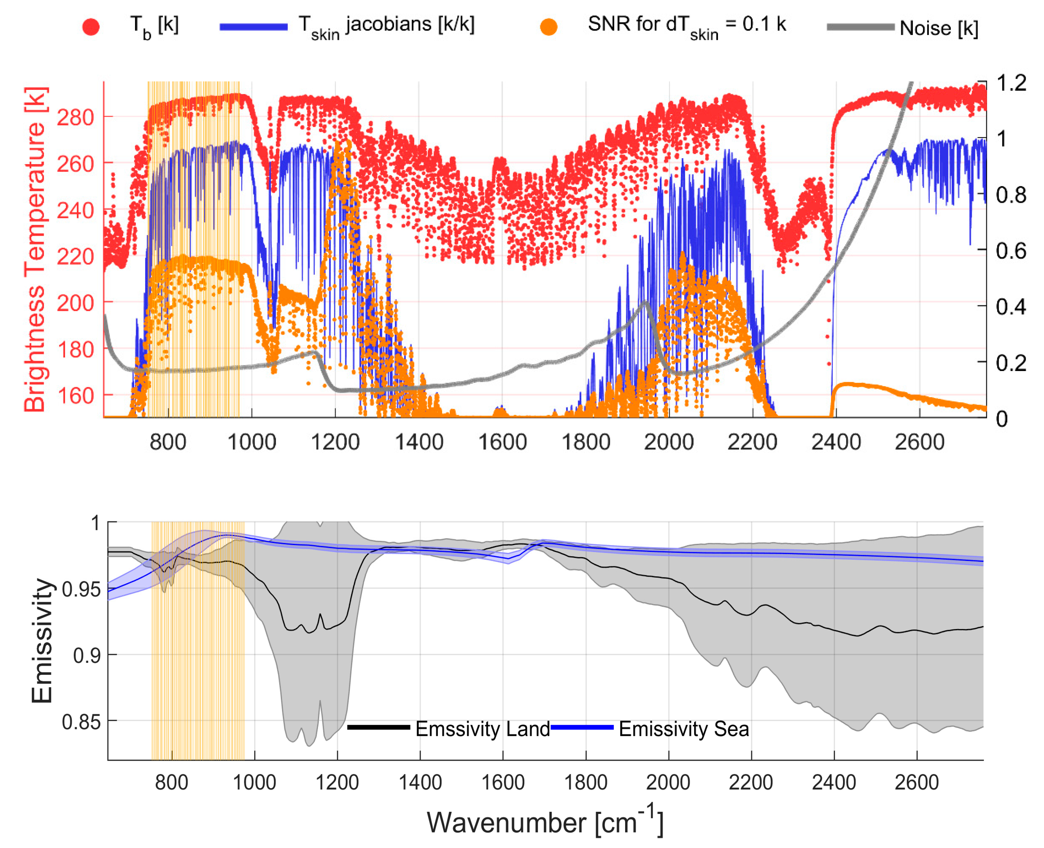
2.1. Choice of IASI Spectral Window for T_skin Retrieval

IASI uses three detectors to fully cover the spectral range that extends from 645 to 2760 cm⁻¹ (15.5 to 3.62 μm) with no gaps. To understand the spectral window that must be used for T_skin retrieval, we show in Figure 1, upper panel, a typical IASI cloud-free spectra, with the corresponding Jacobian (the sensitivity of the IASI brightness temperature to the skin temperature), as well as signal-to-noise ratio (SNR), and radiometric noise. The recorded spectrum, with an example shown in red in the upper panel of Figure 1, in brightness temperature units (K), exhibits signatures associated with spectroscopic absorption/emission lines of molecules present along the optical path between the Earth’s surface and the satellite detectors. From these spectra, geophysical data such as temperature profiles and atmospheric concentrations of trace gases can be retrieved from the selected spectral windows. Channels that are candidates for T_skin retrieval are therefore located in spectral windows with little interference from other absorbing/emitting molecules, and are also those where the T_skin Jacobians (blue line in upper panel) are the highest. These are the spectral ranges before and after the ozone band, i.e., 800–1040 cm⁻¹ and 1080–1150 cm⁻¹, the small spectral window after the water vapor continuum at ~2150 cm⁻¹ and the spectral range >2400 cm⁻¹.

The window >2400 cm⁻¹, as well as that around ~2150 cm⁻¹ may be contaminated by solar radiation during the day. In terms of SNR, the very important values of the radiometric noise at >2400 cm⁻¹ induce a low value of the SNR. The spectral band at ~2150 cm⁻¹ presents a slightly weaker performance than the spectral ranges around the ozone absorption band. These two spectral bands (~2150 and >2400 cm⁻¹) were therefore not critical for the T_skin retrieval and were discarded.

The lower panel of Figure 1 shows the average emissivity over land (in black) and sea (in blue). Emissivity is needed to calculate T_skin from the radiative transfer equation, and it changes as a function of wavenumber, as the figure shows. We can see that on the right of the ozone band, around 1100–1200 cm⁻¹, the variability of the emissivity, especially over land is much more important than the window between 750 and 970 cm⁻¹, where the noise is also smaller, and the SNR higher. This makes this spectral window the best candidate for T_skin retrieval. The yellow thin vertical lines indicate the location of the channels that were used in this study to retrieve skin temperature (a zoomed version is provided in Figure 2) and the description of the retrieval is provided in the following section.

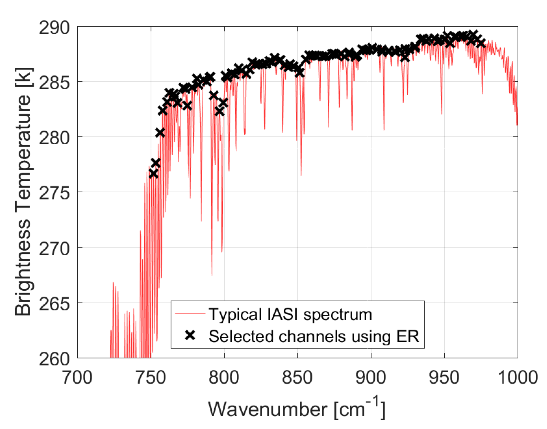
2.2. Channel Selection based on Entropy Reduction

We used an iterative method where channels are selected based on their ability to reduce the uncertainty of retrieving temperature. It was proposed by [34,37], evaluated for IASI by [38] and applied by [35] to Numerical Weather Prediction (NWP). The method has been rigorously studied and relies on evaluating the impact of the addition of single channels on a theoretical retrieval based on a figure of merit, such as the Entropy Reduction (ER), used in this study, and defined as follows:

$$ER=\frac{1}{2}lo{g}_2\left(B{A}^{-1}\right)$$

(1)

$ER$ measures the probabilities of the ensemble of possible states in the retrieval, and is maximal if all the states have an equal probability. The lower the entropy of the ensemble, the better the retrieval. The channel that reduces this entropy emphasizes a particular state of the retrieval. Entropy reduction is a metric derived from information theory, specifically from relative entropy, where two densities are compared [39]. In Equation (1), $A$ is the analysis-error covariance matrix, and $B$ is the background/a priori error covariance matrix, with:

$$A={\left(B^{-1}+H^T{R}^{-1}H\right)}^{-1},$$

(2)

where $H$ is the Jacobian matrix of T_skin and $R$ the covariance matrix of instrumental and radiative transfer noises. External variables such as water vapor or ozone can contaminate a given candidate T_skin channel by absorbing in the targeted spectral range. This might affect the selection, and introduces an error that should be added to the $A$ matrix [40,41]. If those errors were not included in the background $B$ matrix, the quality of the selected channels might be artificially over-estimated. When this contaminating effect is defined explicitly, Equation (2) is updated to:

$$A_{V^{-1}}=B_V^{-1}+H_V^t · {\left(R+H_{\mathsf{\nu }}· B_{\mathsf{\nu }} · H_{\mathsf{\nu }}^t\right)}^{-1}· H_V,$$

(3)

where $V$ is the variable to be retrieved (T_skin) and $\mathsf{\nu }$ is the external variable (e.g., ozone or water vapor). This equation is valid by making some assumptions, in particular that no correlation between $V$ and $\mathsf{\nu }$ exists and that the impact of this external variable contamination on the channel is an error with Gaussian distribution with covariance matrix $H_{\mathsf{\nu }}^t·B_{\mathsf{\nu }}·H_{\mathsf{\nu }}$.

In most channel selection analyses, the errors from external variables (such as that of relative humidity or ozone) are not taken into account in the measurement of the information content of the candidate channel. A study [35] attempted to take into account the effects of trace gases not included in the radiative transfer simulation by inflating the observation errors for channels that showed sensitivity to the missing species. A more complete approach was adopted by [42], who used climatological variability of atmospheric constituent species to model their effect on the radiances during the channel selection process.

In this work, we explicitly considered the contamination effect in the selection process of dedicated T_skin related-channels. This refined methodology improves the representation of contamination effects from atmospheric species and therefore the reliability of the background error covariance matrix $B$. This matrix $B$ characterizes the quality of the a priori information and varies in space and time in order to account for its complex state-dependence. For this work, we derived a Gaussian $B$ matrix as: $B=Cov\left(x,y\right)$ at the vertical level x and y. An uncertainty of $\mathsf{\sigma }$ = 2 K was chosen for T_skin, as done by [35]. The covariance and correlation matrices of the background errors for relative humidity and ozone were calculated based on the widely used assumption that humidity (or ozone) error correlation between the vertical layers is close to the actual associated humidity (or ozone) correlation. We chose to have the covariance matrices $B$ for humidity and ozone based on the raw humidity and ozone correlation matrices, and an error variance (${\mathsf{\sigma }}^2$) of 20% for humidity, and 30% for ozone on each vertical atmospheric layer. As humidity and ozone can impact T_skin channel selection, error along the vertical is needed for T_skin retrieval.

An iterative method [34] was used to forwardly select the most informative channels. In order to speed up the computations, an efficient algorithm was developed assuming that the observation errors are uncorrelated between channels. However, as the IASI radiances are apodized, and thus have highly-correlated errors between adjacent channels, a channel is not selected if its immediate neighbor is already chosen [35].

The iterative procedure was initialized with $A_0=B$, and the Jacobian $H$ (which is constant during the iteration) was normalized with the instrumental noise covariance matrix $R,$ as follows: $H^{\prime }=R^{-1/2}H$.

According to [34], the updated analysis error covariance matrix at each iteration step $i$ can be calculated from the previous step $i-1$ as follows:

$$A_i=A_{i-1}-\frac{\left(A_{i-1}{h}^{\prime }\right){\left(A_{i-1}{h}^{\prime }\right)}^T}{1+{\left(A_{i-1}{h}^{\prime }\right)}^T{h}^{\prime }}$$

(4)

where $h^{\prime }$ is the column vector equal to the row of $H^{\prime }$ for the candidate channel.

The ER change between two iterations can now be written as:

$$\Delta ER=\frac{1}{2}lo{g}_2\left(1+h{\prime }^T{A}_{i-1}{h}^{\prime }\right)$$

(5)

At each step, the channel that has the largest information content (measured as a reduction of the entropy of the corresponding T_skin retrieval when the candidate channel is used) is selected, given the information content of the previously selected channel(s). The channel selection starts with no channel selected, and sequentially chooses the channel with the highest information content in complement to the information from all the previously selected channels.

The spectra and Jacobians used in this study were simulated using the last version of the Optimum Spectral Sampling (OSS) radiative transfer model [43], using the Thermodynamic Initial Guess Retrieval (TIGR3) database [44], and more detailed descriptions on the atmospheric profiles, the radiative transfer code, and the Jacobians, can be found in [45]. Here, a channel selection was only performed over the spectral window of T_skin retrieval, as was discussed in Section 2.1, and is shown in Figure 2. The IASI spectral window was divided into 100 spectral subsets and a channel selection was applied to each. Using this method, we selected the best 100 channels in terms of information content and the resulting selection is listed in

Table 1. The 100 channels used for T_skin retrieval selected using the Entropy Reduction (ER) method. Channels are sorted from the highest to the lowest information content (top to bottom and left to right).

Channel	Wavenumber (cm−1)	Channel	Wavenumber (cm−1)	Channel	Wavenumber (cm−1)	Channel	Wavenumber (cm−1)
1300	969.75	1038	904.25	853	858.00	682	815.25
1282	965.25	1100	919.75	984	890.75	582	790.25
1249	957.00	1001	895.00	862	860.25	630	802.25
1272	962.75	1321	975.00	771	837.50	625	801.00
1254	958.25	1209	947.00	759	834.50	574	788.25
1294	968.25	1069	912.00	752	832.75	584	790.75
1230	952.25	997	894.00	797	844.00	547	781.50
1164	935.75	1070	912.25	745	831.00	551	782.50
1267	961.50	921	875.00	775	838.50	565	786.00
1194	943.25	962	885.25	801	845.00	516	773.75
1179	939.50	1051	907.50	714	823.25	510	772.25
1222	950.25	940	879.75	706	821.25	593	793.00
1311	972.50	916	873.75	698	819.25	534	778.25
1086	916.25	1114	923.25	844	855.75	484	765.75
1157	934.00	950	882.25	726	826.25	472	762.75
1172	937.75	869	862.00	810	847.25	488	766.75
1142	930.25	1237	954.00	736	828.75	494	768.25
1203	945.50	926	876.25	824	850.75	466	761.25
1018	899.25	961	885.00	691	817.50	619	799.50
1141	930.00	875	863.50	669	812.00	609	797.00
1009	897.00	979	889.50	661	810.00	521	775.00
1089	917.00	889	867.00	786	841.25	454	758.25
1115	923.50	899	869.50	827	851.50	447	756.50
1025	901.00	897	869.00	642	805.25	435	753.50
1126	926.25	1052	907.75	650	807.25	429	752.00

and presented in Figure 2. The figure shows that most of the selected channels were between 760 and 980 cm⁻¹. However, few channels were also selected for wavenumbers <760 cm⁻¹ since in this part of the spectrum, the atmospheric vertical levels are very correlated to one another and therefore information on the surface exists in these channels.

2.3. Artificial Neural Network for T_skin Retrievals

The artificial neural networks (ANN) method was used to approximate the complex radiative transfer function that maps the radiances to skin temperature. The feasibility of using ANN to T_skin retrieval has been shown, for instance, by [46] for IASI, and has also been performed to tackle various problems in atmospheric remote sensing [47,48,49,50]. The retrieval, even if trained with the reanalysis, does not reproduce the reanalysis; the time and spatial variations are driven by the satellite observations [51,52,53]. For AIRS and AMSU, projected principal components for coefficient compression and a neural network trained using a global training set derived from European Center for Medium-Range Weather Forecasting (ECMWF) fields are used for retrievals of atmospheric temperatures and water vapor [54,55].

The training dataset was constructed out of clear-sky IASI scenes (cloud cover <10%). ERA5 hourly T_skin reanalysis product [56] of the Copernicus Climate Change Service [57] was used as the output/target.

Clear-sky IASI observations were selected using AVHRR measurements, collocated with those of IASI, both instruments being on Metop [58]. Level 1C (L1C) clear-sky IASI radiances were extracted for the 100 channels Selected in Section 2.2. For the training datasets, one day (the 15th of each month) was chosen from 2008 to 2017. From each file, 10,000 points were randomly selected (for a total of 1.2 million scenes), and then separated between land and sea scenes. Two distinct ANN trainings were performed: one over sea, and one over land. Both ANN trainings were done using mini-batches with a maximum of 10,000 epochs to train. The ANN had two hidden layers with four nodes, and a network training function that updates weight and bias values according to the Levenberg-Marquardt optimization. For both ANNs, ERA5 skin temperature product was used as the target for the training. We provide more information on the ERA5 reanalysis in Section 2.4. In the following, “T_ANN” refers to the product developed in this study using artificial neural networks from IASI radiances.

2.3.1. T_skin Retrievals over Sea

Over sea, the input to the ANN was simply the 100 radiance channels provided in Table 1. For each set of 100 radiances, T_skin from the ERA5 reanalysis was used as the target, co-localized in space and time with IASI’s observation. 3D gridded data interpolation was used. The interpolant was created from ERA5 data (0.25° longitude/latitude grid and 1-h time resolution), using the “griddedInterpolant” function of Matlab. The interpolant was then applied to time, longitude, and latitudes of IASI. Figure 3 shows the training results when T_ANN was compared with T_ERA5 used for the training. As expected, a good agreement was achieved, with a standard deviation of the T_ERA5–T_ANN equal to 0.99, and a correlation coefficient ~1. The largest differences were for points located near the poles. This was probably due to either an incorrect cloud cover detection or to partially ice-covered pixels detected as “sea”. It was also shown that ERA5 data might underestimate winds, and overestimate surface air temperature slightly over the poles [59]. A sea-ice mask is recommended, therefore, when performing temperature comparison studies at high latitudes. Further validation is provided in the following section.

2.3.2. Skin Temperature Retrievals over Land

To retrieve skin temperature over land, we apply a similar approach to that done over sea, but we include information on land surface emissivity. This was done to improve the ANN training in regions where land cover variability/surface properties play an important role in determining skin temperature. We use monthly climatological emissivities from IASI based on the work by [60,61]. The dataset is updated and includes monthly emissivities at a 0.25° × 0.25° grid globally from Metop-A, over the period from 1st June 2007 to 31th May 2017 (10 years). Our tests (not shown here), show that the standard deviation of emissivity reaches 0.002 (0.13 °C) with a global mean of ~5 × 10⁻⁴ at 926.25 cm⁻¹ (0.03 °C).

For each of the scenes selected for the ANN training, we add to the 100 radiance channels the corresponding 100 emissivities at the scene’s longitude and latitude. We train our datasets with the spatio-temporal collocated ERA5 T_skin. Figure 4 shows the results when T_ANN is compared with T_ERA5 used for the training. Since surface properties are more various, the standard deviation over land (T_ERA5–T_ANN = 3.26) is higher than that over sea. Correlation coefficient is close to 1. The largest differences are for points located near the poles’ coast potentially due to pixels that are part land/part sea, and to missed clouds.

2.4. Datasets Used for Validation

We compared sea and land T_ANN datasets to the EUMETSAT L2 product, the ECMWF ERA5 reanalysis, the SEVIRI satellite retrieval, and ground observations. We describe each dataset used briefly hereafter.

2.4.1. EUMETSAT T_skin Product

IASI temperatures (L2 data) from EUMETSAT [62] are provided for nearly all IASI observations by deriving T_skin primarily from IASI for cloud-free scenes and using the Advanced Microwave Sounding Unit (AMSU), and the Microwave Humidity Sounder (MHS) for cloudy scenes [31,32]. AMSU and MHS are multi-channel microwave radiometers, which measure radiances in 15 and 5 discreet frequency channels, respectively, and provide information on various aspects of the Earth’s atmosphere and surface. They both can be used for cloud-contaminated scenes, since they are synchronized with IASI’s scanning. The algorithm is based on the optimal estimation method. Since the algorithm uses data from instruments on board of Metop, the IASI ANN cloud-free radiances used in this study were also co-localized in space and time. For EUMETSAT data, comparison between IASI derived skin temperature and in-situ observations at Gobabeb leads to an agreement within 3.1 K. Metop-A IASI sea surface temperature have a cool bias of −0.35 K (standard deviation 0.35 K) when compared to drifting buoys [63].

2.4.2. ERA5 T_skin Product

In the framework of the ECMWF’s latest reanalysis (ERA5) [56], skin temperature is defined as the temperature of the surface at radiative equilibrium. It is derived from the surface energy balance within the land model in ERA5 and no assimilation of surface skin temperature observations takes place. Radiances, on the other hand, are assimilated. The surface energy balance is satisfied independently for each tile by calculating its skin temperature. The skin layer represents the vegetation layer, the top layer of the bare soil, or the top layer of the snow pack. In order to calculate the skin temperature, the surface energy-balance equation is linearized for each tile, leading to an expression for the skin temperature [64]. Over the ocean, the sea surface temperature (SST) is specified from an analysis provided by the Operational Sea Surface Temperature and Ice Analysis (OSTIA) [65] from September 2007 and prior to that date from the Met Office Hadley Centre HadISST2 product [66]. The SST analysis is a blend of satellite retrievals and in situ observations from ships, and ensures a detailed horizontal distribution from satellite data anchored to the sparse ship observations. The resulting SST fields are therefore calibrated as if they are ship observations, and therefore, they represent bulk SST fields (i.e., measured a few meters deep). Since the ocean skin temperature (<1 mm thickness) might be cooler than the SST because of the turbulent and long wave radiative heat loss to the atmosphere, parameterizations of different near surface ocean effects are included in the code [64]. ERA5 data are at 0.25^° × 0.25^° resolution (native horizontal resolution of ERA5 is ~31km) and are interpolated in time and space to the IASI observation. ERA5 assimilates different datasets, and the dataset is relatively new, and used as a basis for comparison with other datasets. Global accuracies were not found in the literature, but are provided in this work. Its validation in the Southern Antarctic suggests a warm bias of 0.14 °C, with a significant improvement compared to the ERA5 predecessor, ERA-Interim, in particular at high altitudes [59].

2.4.3. SEVIRI T_skin Product

The Spinning Enhanced Visible and Infrared Imager (SEVIRI) onboard the geostationary Meteosat Second Generation (MSG) satellite scans the Earth surface every 15 min and provides observations in 12 spectral channels with a sampling distance of 3 km at nadir. MSG’s nominal position at 0° longitude and SEVIRI’s large field of view (up to 80° zenith angle) allows for frequent observations of a wide area encompassing Africa, most of Europe, and part of South America [67]. The skin temperature (or also called land surface temperature, LST) product (LSA-001) used for validation here [68,69] was retrieved by the EUMETSAT Land Surface Analysis Satellite Application Facility (LSA SAF) with the generalized split-window method, which requires land surface emissivity as input data. IASI and SEVIRI data are spatially co-located when observations from each instrument are less than 5 min apart, and within 0.25 degrees in longitude and latitude. Validation of the SEVIRI LST product shows that the difference with in situ LST usually lies well within ±2.0 °C accuracy [70], however the study also found that the results for daytime and night-time accuracies differ considerably from station to station, depending on such factors as orography, land cover, and surface homogeneity.

2.4.4. Ground Observations

Two sets of ground observations were used for validation. The first was from the Gobabeb wind tower, Namibia (23.551° S 15.051° E) [71]. Gobabeb station is located on the large and homogenous Namib gravel plains [72]. T_skin measurements are obtained once per minute and it is part of the Karlsruhe Institute of Technology (KIT) stations, designed for continuous validation of LST products over several years. The core instruments of KIT’s validation stations are Heitronics KT15.85 IIP infrared radiometers, that measure radiances between 9.6 and 11.5 μm. The temperature resolution is 0.03 K with an uncertainty of ±0.3 K over the relevant range, and high stability with a drift of less than 0.01% per month [73]. Based on in-situ measurements, the surface emissivity of the gravel plains is estimated as 0.944 ± 0.015 for MSG/SEVIRI 10.8 μm channel [72]. During an international inter-comparison campaign, in-situ emissivity spectra were obtained at 49 sample locations distributed across the gravel plains: the results confirm the previously obtained results [74].

The infrared radiance measurements from KIT stations have been successfully used to validate several satellite LST products derived from MODIS [69,75,76], SEVIRI [69,73,76], and a range of sensors [70]. The monitoring capability of KIT’s validation stations was demonstrated by [71] for LST derived from MSG/SEVIRI. Reference [73] showed that the Gobabeb station T_skin is representative for an area of several 100 km², making it suitable for validation with satellite measurements, and in particular IASI.

The second set of T_skin validation stations was derived from radiative fluxes measured at the Surface Radiation Budget Network (SURFRAD) in the United States [77,78] (https://www.esrl.noaa.gov/gmd/grad/surfrad/). Seven SURFRAD stations are operating in diverse land-type regions in the US and are representative of various land cover types. Details on the stations are listed in

Table 2. List of Surface Radiation Budget Network (SURFRAD) validation sites used in this study.

Site Location	Latitude	Longitude	Surface Emissivity
Table Mountain, CO	40.126° N	105.238° W	0.973
Bondville, IL	40.051° N	88.373° W	0.976
Goodwin Creek, MS	34.255° N	89.873° W	0.975
Fort Peck, MT	48.308° N	105.102° W	0.979
Desert Rock, NV	36.623° N	116.020° W	0.966
Penn State U., PA	40.720° N	77.931° W	0.972
Sioux Falls, SD	43.734° N	96.623° W	0.978

. To derive T_skin, the upwelling (F↑) and down-welling (F↓) thermal infrared radiances, which are measured by two pyrgeometers (spectral range 3.5 to 50.0 µm) are used. These fluxes are related to skin temperature as follows: F↑ = εσT_skin⁴ + (1 − ε) F↓, where ε is the surface emissivity, σ is the Stefan-Boltzmann constant = 5.669 × 10⁻⁸ J m⁻² s⁻¹ K⁻⁴. Surface emissivities at each of the stations are listed in Table 2, based on [77]. Heidinger et al. [79] showed that a 0.1 error in emissivity equates to an error in the SURFRAD skin temperature not exceeding 0.25 K. Our tests (not shown here), also suggested a similar result.

Instrumental error leads to an uncertainty in retrieved skin temperature of less than 1 K [80]. Measurements from SURFRAD have been used for evaluating land surface temperature from a variety of instruments, such as ASTER, MODIS, among others [80,81,82,83].

3. Results

To validate our T_ANN product, the year of 2016 was chosen. T_ANN was calculated from the two ANNs over land and sea obtained in Section 2 by applying it to each set of 100 radiances over sea and into 100 radiances and 100 emissivities over land. All scenes used were IASI cloud-free observations.

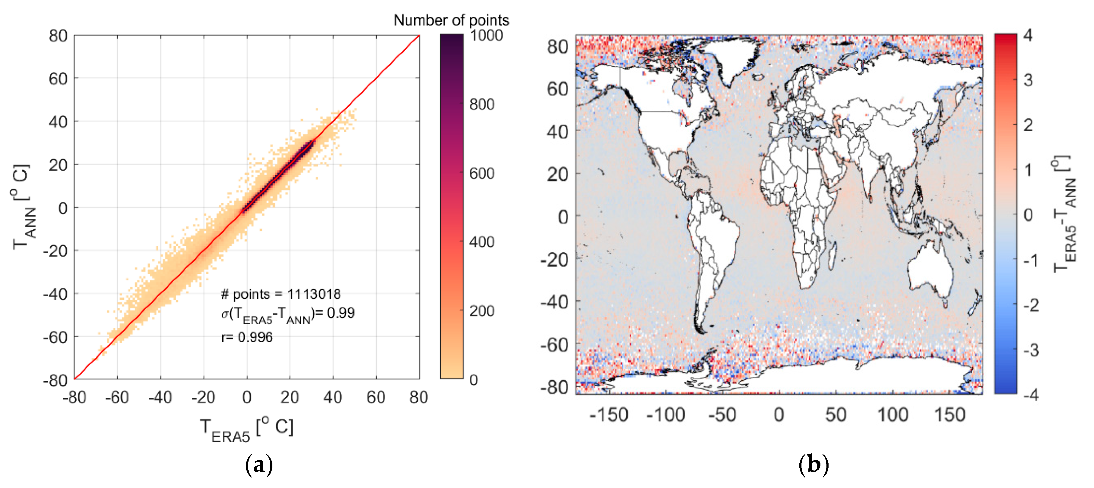
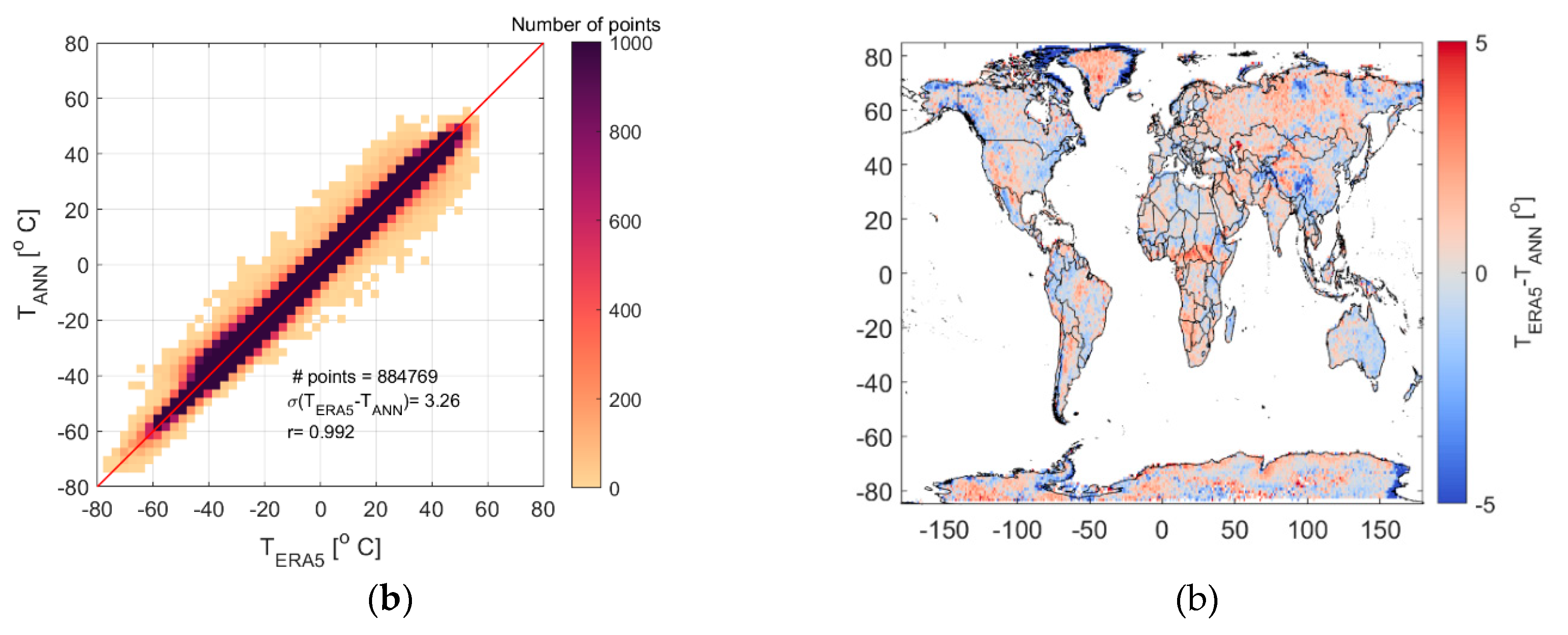
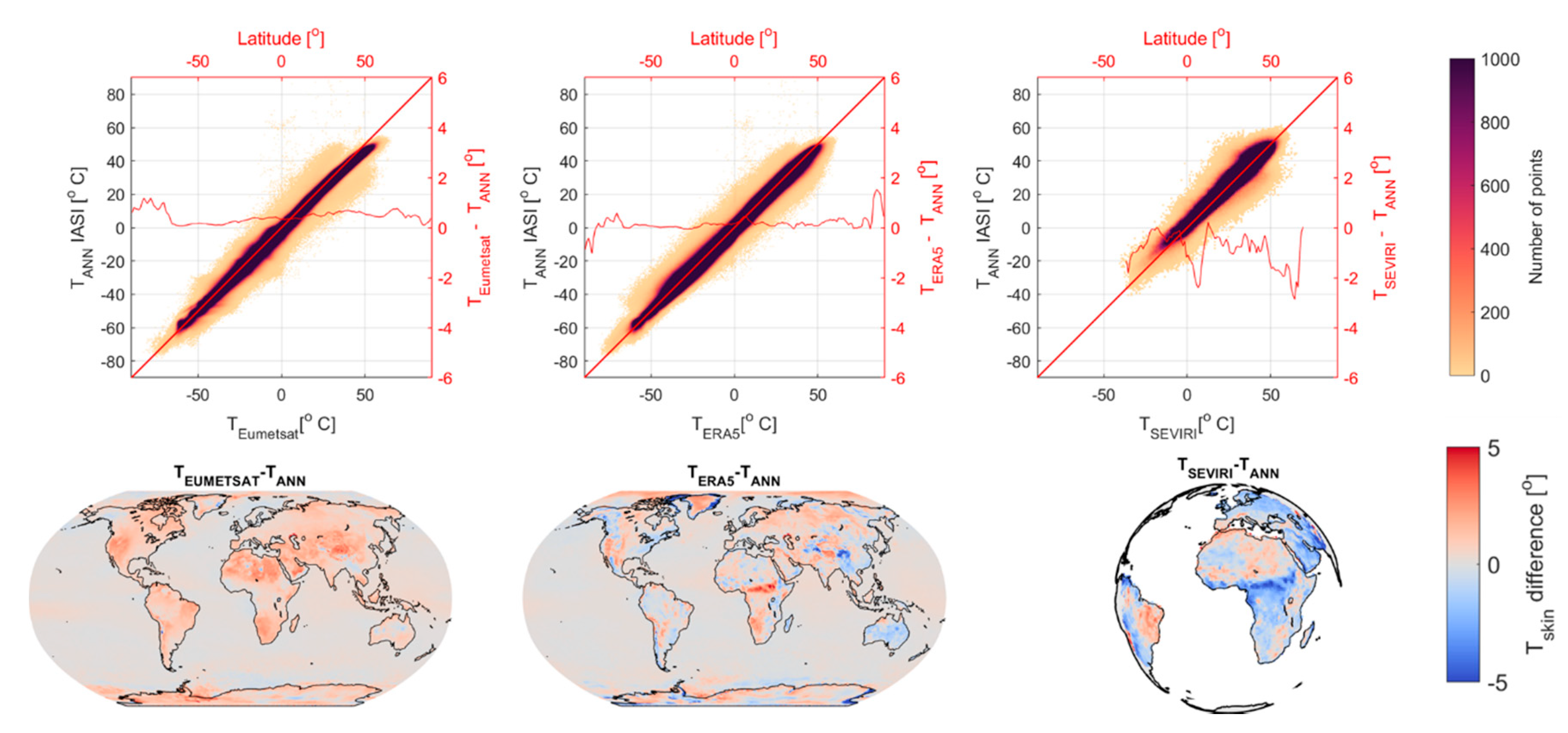
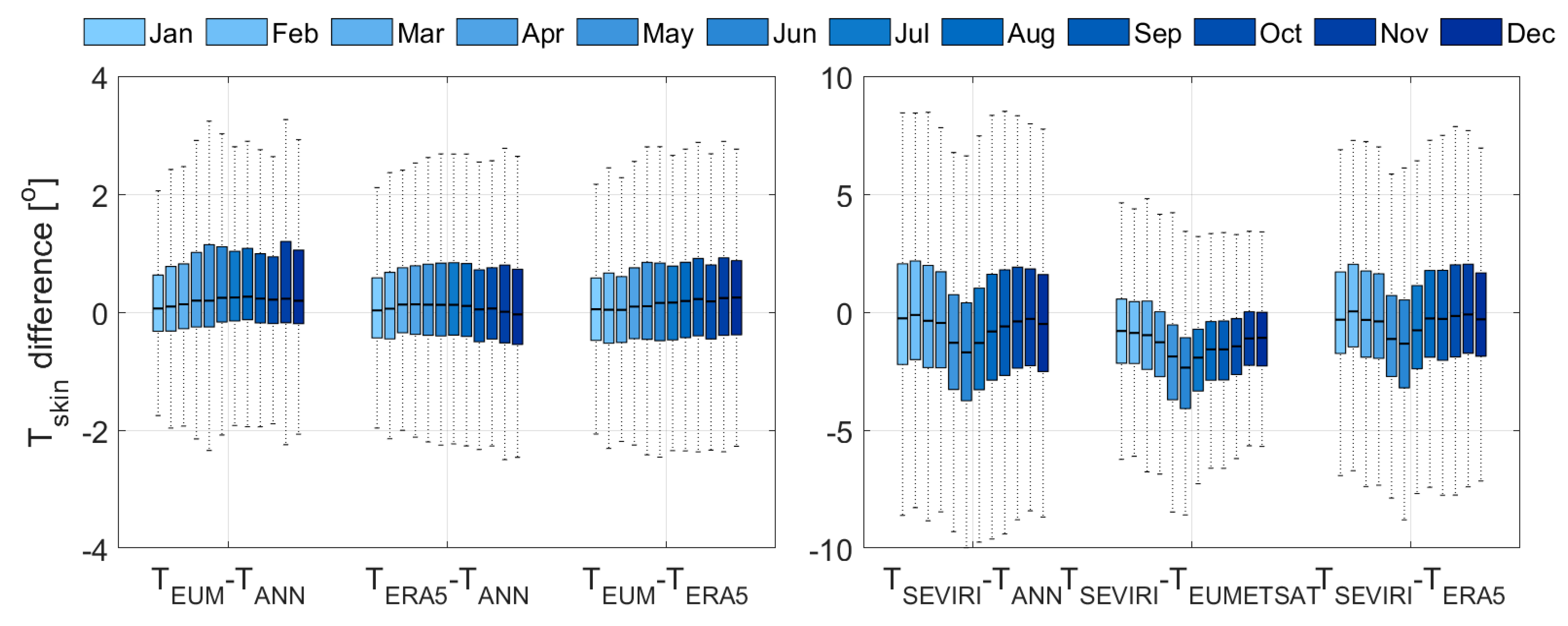
3.1. Validation of T_ANN with ERA5, EUMETSAT and SEVIRI T_skin Products

We started by performing the validation of our T_ANN product with the EUMETSAT, ERA5, and SEVIRI T_skin datasets over the whole 2016 year. The upper panel of Figure 5 shows the correlation plots, superimposed with the average difference by latitude in red. Over the sea, the comparison of our dataset with the skin temperature from ERA5 and EUMETSAT showed excellent results. Over land, positive bias was observed when our T_ANN product was compared with that from EUMETSAT. This has been already seen when EUMETSAT data are validated with ground-based measurement [32], and when they are compared to ERA5 [84]. T_ANN from IASI compared best with the EUMETSAT T_skin product (standard deviation σ = 1.86 °C), which is logical since it was also obtained from IASI radiances. Comparison with ERA5 also showed a correlation close to 1, and σ = 2.10 °C. Globally, and over land, the two datasets agree very well, with the highest differences recorded over the Equator (variable land cover). For the comparisons between T_ANN IASI and T_skin SEVIRI a standard deviation of σ = 3.56 K was determined, with the largest differences over the Arabian Peninsula and the Equator. For large viewing angles, in particular near the edge of the Meteosat disk (the Meteosat is shown here for the comparison with SEVIRI), the uncertainty of SEVIRI T_skin was high [69]. A study [85] reported similar to larger cool biases in the rest of the domain between the ECMWF model data and SEVIRI, especially over semiarid regions, such as North Africa, Sahara, and Namibia. In the rest of the domain, the two datasets agree well.

While this paper focuses on validating IASI T_ANN, inter-comparisons between the different products (ERA5 with EUMETSAT L2 or EUMETSAT L2 with SEVIRI, etc.) are valuable for assessing their differences. Figure 6 shows the box plot of these monthly inter-comparisons during 2016. It can be seen that the T_ANN product developed in the framework of this study is within the range of biases among the other products comparison. Figure 6, left panel, shows that the inter-comparisons of T_ANN, T_EUMETSAT, and T_ERA5 are similar on a monthly basis and the median close to zero. Seasonally, we see that the EUMETSAT T_skin product records a systematic monthly positive bias to our T_ANN product, and to ERA5. Comparison of the Metop-A EUMETSAT skin temperature to that of ERA5 at different latitude bands shows similar results [84]. When we compare our T_ANN product to that of ERA5 seasonally, we can see that the differences are slightly higher in summer, but globally the 25th and 75th percentiles of differences are well below 2 degrees.

Comparison with SEVIRI shows a consistent negative bias when compared to T_ANN, T_EUMETSAT, and T_ERA5, and a seasonal behavior in the differences that are larger in summer. Several studies, e.g., [86,87] already reported cold biases between SEVIRI and other T_skin products. For the ECMWF model, the cold bias over land was identified for a previous version of the model by [88] and for a more recent version by [85]. A misrepresentation of surface energy fluxes, either because of deficiencies in the parameterization of aerodynamic resistances, or in the partitioning between latent and sensible heat fluxes are frequent causes of these deviations [85].

3.2. Validation of the T_ANN with Ground-Based Measurements

For validation with ground measurements, we used the two station datasets mentioned in Section 2.4.4 for 2016.

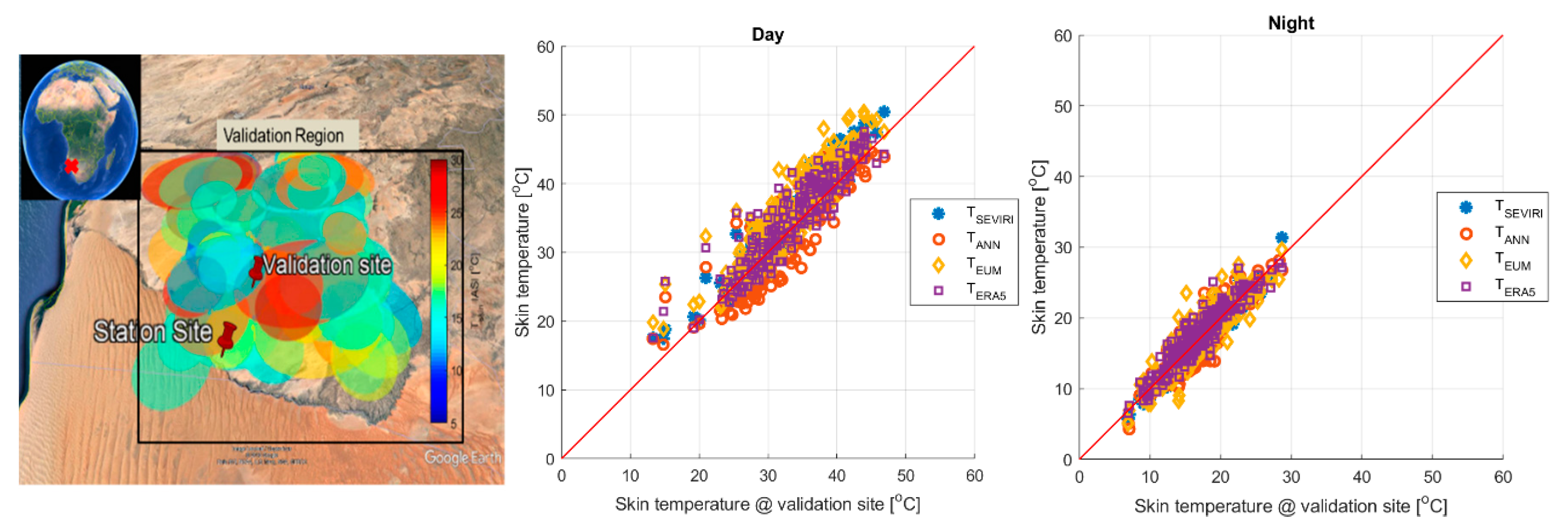
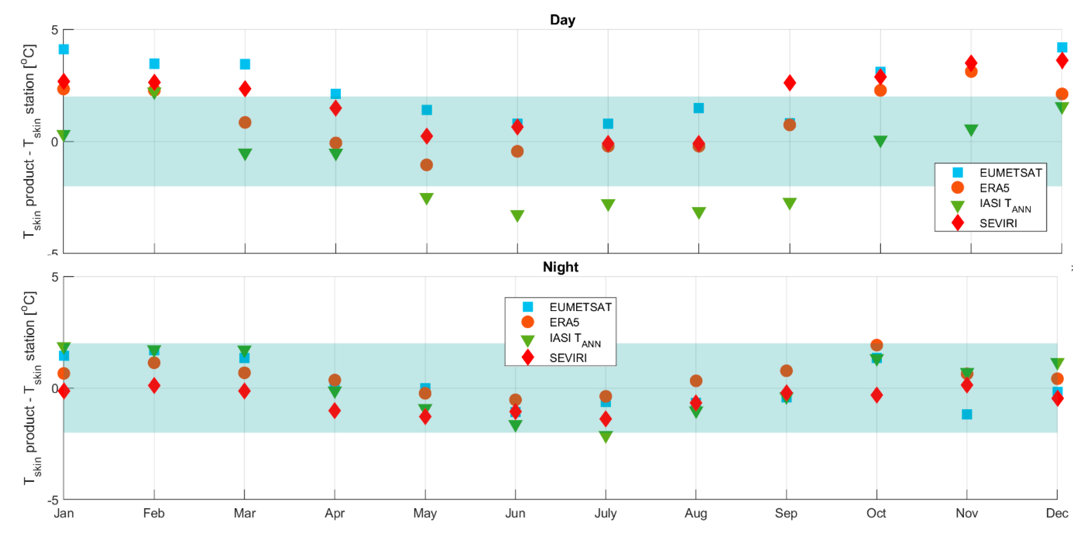
3.2.1. Validation at the Gobabeb Site

First, we show the validation with the Gobabeb site in Namibia. This site was chosen in order to minimize complications from spatial scale mismatch between ground-based and satellite sensors. IASI (and co-localized EUMETSAT and ERA5 and SEVIRI T_skin products) cloud-free data were matched in space and time (within 1 minute of the station data). The spatial matching was done around 0.25° of a validation site [15.17° E, 23.18° S], the location of which is shown in Figure 7. This validation location was chosen because it is close of the station site and is representative of the same gravel plain surface, yet, away from the sand dunes limiting the station. The total number of coincident IASI data points around this area is 446 during the day and 650 during the night. The validation of the T_ANN with in situ T_skin are illustrated in Figure 7 and Figure 8.

Day and night correlation coefficients between the different datasets are > 0.9.

Table 3. 2016 standard deviation and accuracy (median bias) between ground-based station temperature (T_station) and skin temperature from the different datasets used in this study.

	Day		Night
	Standard Deviation [°]	Accuracy [°]	Standard Deviation [°]	Accuracy [°]
TANN–Tstation	2.87	−0.51	1.94	0.03
TEUMETSAT–Tstation	2.80	2.76	1.87	−0.07
TERA5–Tstation	2.65	1.16	1.36	0.40
TSEVIRI–Tstation	1.88	2.25	1.04	−0.56

lists how the different datasets used for validation compare to ground measurements. Accuracies are described using the median accuracy (skin temperature from the different products − skin temperature at the station), as described by [89]. Accuracies’ monthly evolutions are also shown in Figure 8 for daytime (upper panel), and nighttime (lower panel) coincident IASI observations. During the day, the scatter plots in Figure 7, and the monthly median accuracies shown in Figure 8 suggest higher variability. The standard deviation of the differences between the different datasets (in Table 3) show higher values, which is expected since meteorology and cloud cover play a more important role in the daytime variability. The in situ measurement site might be partly cloudy/clear, while the validation site might not. At night, and for all products, comparison with ground measurements is better. It is worth noting here that the numbers discussed in Figure 8 and Table 3 are based on the validation of the T_skin product at the IASI’s crossing time around 9:30 AM and PM. SEVIRI and ERA5 provide T_skin at 15-minute and one-hour resolution, respectively, and validation of these products has been detailed and provided by [70,73] for SEVIRI at Gobabeb, and partly in [90] for ERA5. Martin et al. [70] have shown that the median accuracy for SEVIRI is usually within 2 degrees when compared to Gobabeb station data. Here, we achieved this accuracy only in autumn/winter (March to September) during the daytime, and all year during the nighttime.

During the daytime, the EUMETSAT product overestimated the skin temperature. This has been already noted in a EUMETSAT validation report for both Metop A and Metop B [63]. SEVIRI data also did not achieve the desired accuracy for seven months of the year during the day, which is unusual, since validation of SEVIRI at Gobabeb shows that 2 °C accuracy is achieved [71]. In fact, the full SEVIRI data record comparison with Gobabeb (not shown here) achieves the 2 °C accuracy. The lack of accuracy here is due to the fact that the comparison was made at the crossing time of IASI (around ~9:30 a.m. for the daytime measurements), and the combination of lower number of points, morning fog on gravel plains, and issues with the cloud mask or shadowing effects might be affecting the comparison. Our T_ANN product and that of ERA5 agreed the best with the ground station. While IASI T_ANN was “derived” from the training with the ERA5 product, we can see that they do not behave similarly when validated at the ground station, which is plausible and implies that indeed the variability seen is proper to each of the products. At night, all investigated data sets were generally in good agreement with the ground station data. The differences were all within the 2.0 °C range.

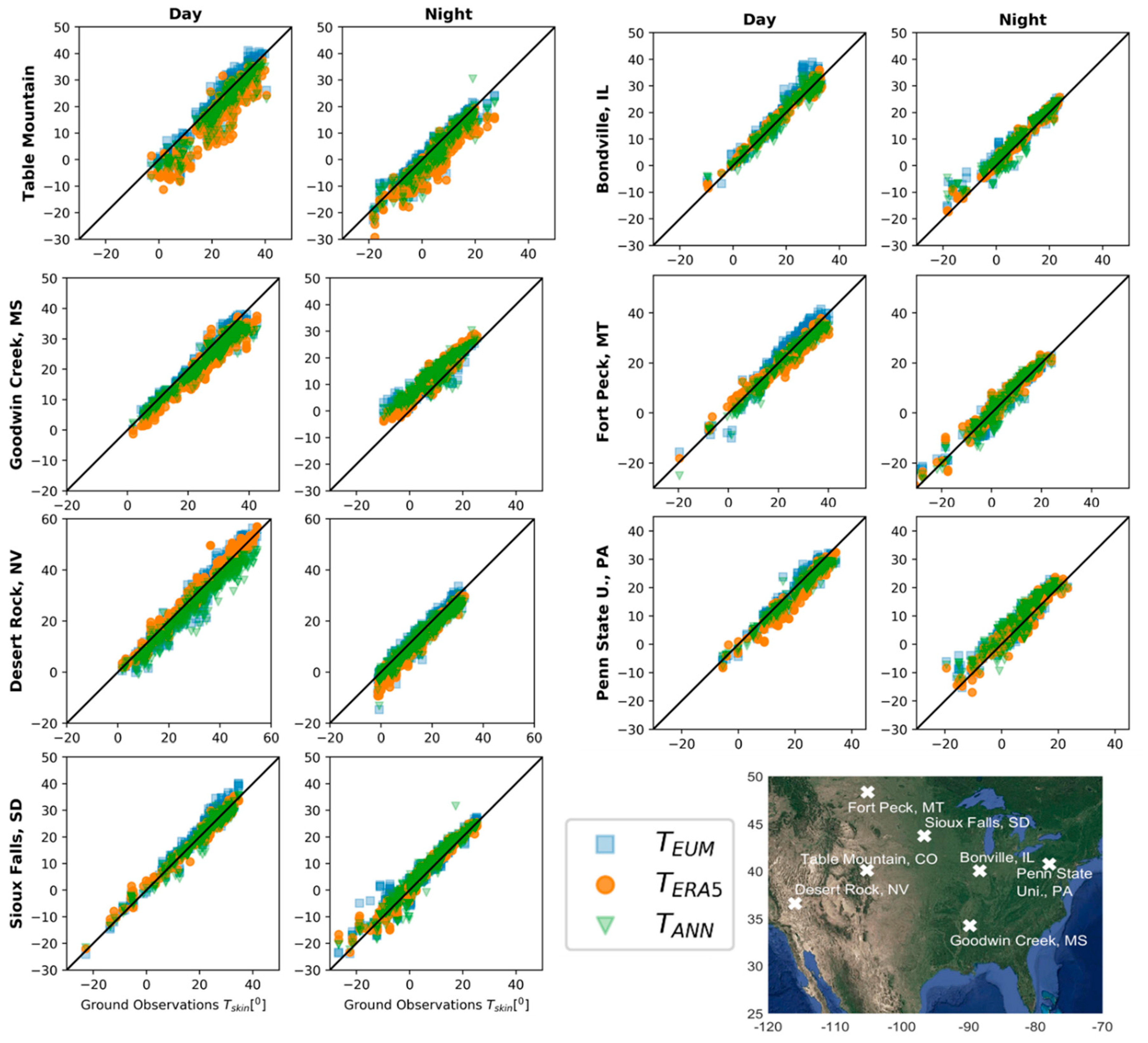
3.2.2. Validation at the SURFRAD Station

IASI cloud-free data were co-localized in space and time within 1 minute of each of the SURFRAD station data. The spatial matching was done at ±0.25° around each of the station (Table 2 and Figure 9). Figure 9 shows the comparison between the skin temperature retrieved from the SURFRAD stations with that of EUMETSAT, ERA5, and our T_ANN product. The station locations are shown in the figure, and they clearly cover different land types.

Figure 9 shows that the three datasets are reasonably correlated with the station data. ERA5 data seem to have most of the outliers, particularly at Table Mountain (for both day and night). To investigate the differences, we separated day and night observations. The median of the differences (the accuracy as was done at Gobabeb station) between the three datasets and T_skin at the station is shown in Figure 10, upper panel, for daytime observations and in the lower panel for nighttime observations. The standard deviation of the differences (not shown here) varies between 1.5 °C (Bondville), and is larger than 4 at the Table Mountain station. Four out of the seven stations shown here are located in areas with heterogeneous land covers, these are Table Mountain, Goodwin Creek, Fort Peck, and Penn State University. The mixture of land cover types found around these stations strongly influences the validation. Moreover, the spatial representativeness of T_skin derived from SURFRAD station is only about 70 × 70 m² [80]. IASI’s and ERA5’s respective resolutions are much coarser and one observation of each contains various land cover types.

For example, the Table Mountain station is located on a mountain slope, and its surroundings are a highly heterogeneous mixture of agricultural fields. The incorrect simulation of surface properties might be responsible for the high ERA5 bias [64] detected at this station. The Goodwin Creek station is located on grass in a rural pasture land in Mississippi. Reference [70] showed with Google Earth imagery that a mixture of forest and grassland is found around the station. This station had the highest bias at night for the three datasets. The other stations agreed reasonably well with the different datasets, and our T_ANN product was within the range of the other two datasets. One of the issues hindering proper comparison might be due to local emissivity differences. We tested this by calculating the skin temperature at each of the stations using our climatological monthly emissivities from IASI, and the results changed by less than 1% annually, with a difference less than 0.25 °C.

The accuracy and standard deviation (accuracy; STDE) for T_ANN–T_SURFRAD, T_ERA5–T_SURFRAD, and T_EUMETSAT–T_SURFRAD for all the stations combined are listed in

Table 4. 2016 standard deviation and accuracy (median bias) between SURFRAD derived T_skin for the seven stations used in this study, and skin temperature from our ANN product, EUMETSAT, and ERA5.

	Day		Night
	Standard Deviation (°)	Accuracy (°)	Standard Deviation (°)	Accuracy (°)
TANN–TSURFRAD	3.32	−2.16	3.67	0.31
TEUMETSAT–TSURFRAD	3.20	0.15	3.20	0.59
TERA5–TSURFRAD	3.53	−1.36	3.71	−0.06

. The standard deviation of the differences was between 3.20 and 3.71 for all datasets. Our T_ANN product achieved a reasonable accuracy of −2.16 °C during the day, and of 0.31 °C at night.

4. Discussion and Conclusions

Satellite data are able to provide systematic global temperature data, at least in cloud-free areas, from pole to pole on a regular basis. EUMETSAT has been updating different versions of algorithms to retrieve the skin temperature from IASI, and at the same time, relying on different instruments (particularly for cloudy scenes) to derive a T_skin product. Consequently, no homogenous consistent IASI T_skin record exists to date. However, in this study we took advantage of the fact that the Metop-A L1C radiances, recently reprocessed at EUMETSAT and used in this work, are homogeneous.

In this study, we derived a T_skin product using Metop-A IASI L1C radiances. The first challenge was to find the channels with access to surface information. To this end, we present a method based on entropy reduction, to find the channels with the highest information content in skin temperature. An efficient and fast IASI retrieval algorithm based on artificial neural networks was then used to calculate T_skin from the upwelling IASI radiances. While empirical methods using ANN can deal with hundreds to thousands of channels [46], we show in this study how ANN and channel selection can be used to retrieve T_skin, making this method fast and reliable for near real-time application, as well as to reprocess more than 13 years of IASI data. In this study, we performed two ANN trainings with IASI radiances, one over land by adding land surface emissivity for each radiance channel, and another training over the sea using only radiances as input. ERA5 hourly simulation was used as the output. The resulting neural networks were then applied for the year 2016 and validated. Our results show the potential of ANN in mapping radiances and emissivities globally and locally to skin temperature [91]. We achieved good correlation when we compared our datasets to other widely used skin temperature datasets, as well as when we compared it to ground measurements. When we compared our T_skin product with that of other datasets, a mean bias and STDE (i.e., [bias, STDE]) of [0.55, 1.86 °C], [0.19, 2.10 °C], [−1.5, 3.56 °C], was found from EUMETSAT IASI L−2 product, ERA5, and SEVIRI. We performed a more detailed statistical analysis when we compared with ground measurements. First, when we compared with Gobabeb station data, the location of which is in the Namibian desert, we found that we achieved at nighttime the required the 2 °C accuracy needed for climate trends construction. At the SURFRAD’s network stations, which cover different locations in the United states, we found that the accuracy found largely depends on the location of the station. The bias was the largest when the IASI or ERA5 coincident observation was over a heterogeneous land cover. On average, we were able to achieve the 2 °C accuracy at four out of the seven stations. Our product’s accuracy is within the accuracy and standard deviation of the other products.

More generally, retrieval of T_skin from space measurements faces many challenges. The solution of the radiative transfer equation requires the simultaneous knowledge of two unknowns: T_skin and the surface emissivity. In our study this was accounted for, since emissivity was used as the input to the ANN over land. Second, infrared retrievals are only available under clear-sky conditions, reducing the amount of global data by roughly one-third. This study has been performed with data from IASI on Metop A, and it implies that with IASI on Metop B and Metop C, the global coverage can be enhanced during their overlapping periods. Third, validation and inter-comparison between different products are challenges that are not only bound to this study. The diversity in sensor characteristics and sensor-specific skin temperature retrieval algorithms, as well as the different challenges facing current NWP models, make it difficult to homogenize different skin temperature products for proper comparison. Moreover, for polar-orbiting satellite products, inter-comparison between different T_skin satellite products is challenging, since the crossing times of the satellites and the shape of the field of view are different. For example, MODIS (with overpass time at 10:30 a.m./p.m. on TERRA) and MODIS and AIRS, on the AQUA platform (with an overpass time of 1:30 a.m./p.m.), both offer a good skin temperature product. IASI, on the other hand, has an overpass time of 9:30 am/pm local-time. Since skin temperature, particularly over the land surfaces, vary strongly in space and time [92], inter-comparison between IASI and MODIS or AIRS, with a time difference of one to more than four hours can imply a difference of the order of 10 degrees or more in some regions. This makes inter-comparison with other satellite products with different crossing times very difficult to achieve. Moreover, considering IASI’s pixel area at nadir and at its outermost viewing angle of 48° (off-nadir), several surface types with varying skin temperature and emissivities will co-exist within one pixel. The resulting skin temperature is therefore an “effective” measure of the average of the surface-heterogeneity existing in the pixel. This alone complicates the physical understanding of the T_skin values retrieved from space from different instruments with different pixel shapes (round/ellipse vs. square/rectangle, etc.), and sizes. Moreover, the satellite viewing angle also plays a role in the T_skin at the surface: the comparison is affected by the different Sun–surface–instrument geometries, as a result of shadows due to orography or vegetation, for example [62].

Using channel selection and artificial neural network, this work showed a T_skin retrieval method that can serve as a baseline for constructing the first homogeneous dataset of skin temperature from IASI, and can be extended to other infrared remote measurements. Future work will look at constructing a T_skin time series from IASI during 2007-present and using Metop A, B, and C for climate trends application. Regional and seasonal variations can be studied using the atlas for the surface skin temperature distributions. The daily/monthly/yearly variations will be studied in terms of the main climate drivers (solar, volcanic eruptions, aerosols, and greenhouse gases) and modes of variability at the inter-annual and decadal timescales.

References

1. Goldberg, M.D.; Qu, Y.; McMillin, L.M.; Wolf, W.; Zhou, L.; Divakarla, M. AIRS near-real-time products and algorithms in support of operational numerical weather prediction. IEEE Trans. Geosci. Remote Sens. 2003, 41, 379–389. [Google Scholar] [CrossRef]
2. Zhou, L.; Dickinson, R.E.; Tian, Y.; Jin, M.; Ogawa, K.; Yu, H.; Schmugge, T. A sensitivity study of climate and energy balance simulations with use of satellite-derived emissivity data over Northern Africa and the Arabian Peninsula. J. Geophys. Res. Atmos. 2003, 108, 4795. [Google Scholar] [CrossRef] [Green Version]
3. Rhee, J.; Im, J.; Carbone, G.J. Monitoring agricultural drought for arid and humid regions using multi-sensor remote sensing data. Remote Sens. Environ. 2010, 114, 2875–2887. [Google Scholar] [CrossRef]
4. Becker, F.; Li, Z. Surface temperature and emissivity at various scales: Definition, measurement and related problems. Remote Sens. Rev. 1995, 12, 225–253. [Google Scholar] [CrossRef]
5. McKeown, W.; Bretherton, F.; Huang, H.L.; Smith, W.L.; Revercomb, H.L. Sounding the Skin of Water: Sensing Air–Water Interface Temperature Gradients with Interferometry. J. Atmos. Ocean. Technol. 1995, 12, 1313–1327. [Google Scholar] [CrossRef] [Green Version]
6. Prigent, C.; Aires, F.; Rossow, W.B. Land surface skin temperatures from a combined analysis of microwave and infrared satellite observations for an all-weather evaluation of the differences between air and skin temperatures. J. Geophys. Res. Atmos. 2003, 108, 4310. [Google Scholar] [CrossRef]
7. Prigent, C.; Aires, F.; Rossow, W.B. Retrieval of Surface and Atmospheric Geophysical Variables over Snow-Covered Land from Combined Microwave and Infrared Satellite Observations. J. Appl. Meteorol. 2003, 42, 368–380. [Google Scholar] [CrossRef] [Green Version]
8. Good, E.J. An in situ-based analysis of the relationship between land surface “skin” and screen-level air temperatures. J. Geophys. Res. Atmos. 2016, 121, 8801–8819. [Google Scholar] [CrossRef]
9. Trigo, I.F.; Peres, L.F.; DaCamara, C.C.; Freitas, S.C. Thermal Land Surface Emissivity Retrieved From SEVIRI/Meteosat. IEEE Trans. Geosci. Remote Sens. 2008, 46, 307–315. [Google Scholar] [CrossRef]
10. Jin, M. Analysis of Land Skin Temperature Using AVHRR Observations. Bull. Am. Meteorol. Soc. 2004, 85, 587–600. [Google Scholar] [CrossRef]
11. Wan, Z.; Li, Z. A physics-based algorithm for retrieving land-surface emissivity and temperature from EOS/MODIS data. IEEE Trans. Geosci. Remote Sens. 1997, 35, 980–996. [Google Scholar] [CrossRef]
12. Ruzmaikin, A.; Aumann, H.H.; Lee, J.; Susskind, J. Diurnal Cycle Variability of Surface Temperature Inferred From AIRS Data. J. Geophys. Res. Atmos. 2017, 122, 10928–10938. [Google Scholar] [CrossRef]
13. Siméoni, D.; Singer, C.; Chalon, G. Infrared atmospheric sounding interferometer. Acta Astronaut. 1997, 40, 113–118. [Google Scholar] [CrossRef]
14. Blumstein, D.; Chalon, G.; Carlier, T.; Buil, C.; Hebert, P.; Maciaszek, T.; Ponce, G.; Phulpin, T.; Tournier, B.; Simeoni, D.; et al. IASI Instrument: Technical Overview and Measured Performances. In Infrared Spaceborne Remote Sensing XII; International Society for Optics and Photonics: Washington, DC, USA, 2004; Volume 5543, pp. 196–207. [Google Scholar]
15. Hilton, F.; Armante, R.; August, T.; Barnet, C.; Bouchard, A.; Camy-Peyret, C.; Capelle, V.; Clarisse, L.; Clerbaux, C.; Coheur, P.-F.; et al. Hyperspectral Earth Observation from IASI: Five Years of Accomplishments. Bull. Am. Meteorol. Soc. 2012, 93, 347–370. [Google Scholar] [CrossRef]
16. Collard, A.D.; McNally, A.P. The assimilation of Infrared Atmospheric Sounding Interferometer radiances at ECMWF. Q. J. R. Meteorol. Soc. 2009, 135, 1044–1058. [Google Scholar] [CrossRef]
17. Clerbaux, C.; Boynard, A.; Clarisse, L.; George, M.; Hadji-Lazaro, J.; Herbin, H.; Hurtmans, D.; Pommier, M.; Razavi, A.; Turquety, S.; et al. Monitoring of atmospheric composition using the thermal infrared IASI/MetOp sounder. Atmos. Chem. Phys. 2009, 9, 6041–6054. [Google Scholar] [CrossRef] [Green Version]
18. Coheur, P.-F.; Clarisse, L.; Turquety, S.; Hurtmans, D.; Clerbaux, C. IASI measurements of reactive trace species in biomass burning plumes. Atmos. Chem. Phys. 2009, 9, 5655–5667. [Google Scholar] [CrossRef] [Green Version]
19. Clarisse, L.; R’Honi, Y.; Coheur, P.-F.; Hurtmans, D.; Clerbaux, C. Thermal infrared nadir observations of 24 atmospheric gases. Geophys. Res. Lett. 2011, 38, L10802. [Google Scholar] [CrossRef] [Green Version]
20. Clerbaux, C.; Hadji-Lazaro, J.; Turquety, S.; George, M.; Boynard, A.; Pommier, M.; Safieddine, S.; Coheur, P.-F.; Hurtmans, D.; Clarisse, L.; et al. Tracking pollutants from space: Eight years of IASI satellite observation. C. R. Geosci. 2015, 347, 134–144. [Google Scholar] [CrossRef]
21. Clerbaux, C.; Hadji-Lazaro, J.; Turquety, S.; Mégie, G.; Coheur, P.-F. Trace gas measurements from infrared satellite for chemistry and climate applications. Atmos. Chem. Phys. 2003, 3, 1495–1508. [Google Scholar] [CrossRef] [Green Version]
22. Brindley, H.; Bantges, R.; Russell, J.; Murray, J.; Dancel, C.; Belotti, C.; Harries, J. Spectral Signatures of Earth’s Climate Variability over 5 Years from IASI. J. Clim. 2015, 28, 1649–1660. [Google Scholar] [CrossRef]
23. Smith, N.; Smith, W.L.; Weisz, E.; Revercomb, H.E. AIRS, IASI, and CrIS Retrieval Records at Climate Scales: An Investigation into the Propagation of Systematic Uncertainty. J. Appl. Meteorol. Clim. 2015, 54, 1465–1481. [Google Scholar] [CrossRef]
24. Whitburn, S.; Clarisse, L.; Bauduin, S.; George, M.; Hurtmans, D.; Safieddine, S.; Coheur, P.F.; Clerbaux, C. Spectrally Resolved Fluxes from IASI Data: Retrieval Algorithm for Clear-Sky Measurements. J. Clim. 2020, 33, 6971–6988. [Google Scholar] [CrossRef] [Green Version]
25. Zhou, D.K.; Larar, A.M.; Liu, X. Global Surface Skin Temperature Analysis from Recent Decadal IASI Observations. In Multispectral, Hyperspectral, and Ultraspectral Remote Sensing Technology, Techniques and Applications VII; International Society for Optics and Photonics: Washington, DC, USA, 2018; Volume 10780, p. 1078005. [Google Scholar]
26. Brindley, H.E.; Bantges, R.J. The Spectral Signature of Recent Climate Change. Curr. Clim. Chang. Rep. 2016, 2, 112–126. [Google Scholar] [CrossRef] [Green Version]
27. Susskind, J.; Schmidt, G.A.; Lee, J.N.; Iredell, L. Recent global warming as confirmed by AIRS. Environ. Res. Lett. 2019, 14, 044030. [Google Scholar] [CrossRef]
28. CLERBAUX, C.; CREVOISIER, C. New Directions: Infrared remote sensing of the troposphere from satellite: Less, but better. Atmos. Environ. 2013, 72, 24–26. [Google Scholar] [CrossRef]
29. Crevoisier, C.; Clerbaux, C.; Guidard, V.; Phulpin, T.; Armante, R.; Barret, B.; Camy-Peyret, C.; Chaboureau, J.-P.; Coheur, P.-F.; Crépeau, L.; et al. Towards IASI-New Generation (IASI-NG): Impact of improved spectral resolution and radiometric noise on the retrieval of thermodynamic, chemistry and climate variables. Atmos. Meas. Tech. 2014, 7, 4367–4385. [Google Scholar] [CrossRef] [Green Version]
30. Klaes, K.D.; Cohen, M.; Buhler, Y.; Schlüssel, P.; Munro, R.; Luntama, J.-P.; von Engeln, A.; Clérigh, E.Ó.; Bonekamp, H.; Ackermann, J.; et al. An Introduction to the EUMETSAT Polar system. Bull. Am. Meteorol. Soc. 2007, 88, 1085–1096. [Google Scholar] [CrossRef]
31. EUMETSAT IASI Level 1: Product Guide; EUM/OPS-EPS/MAN/04/0032 2017; EUMETSAT: Darmstadt, Germany, 2017.
32. EUMETSAT IASI Level 2: Product Guide; EUM/OPS-EPS/MAN/04/0033 2017; EUMETSAT: Darmstadt, Germany, 2017.
33. EUMETSAT IASxxx1C0100IASI Level 1C Climate Data Record Release 1-Metop-A; EUMETSAT: Darmstadt, Germany, 2018. [CrossRef]
34. Rodgers, C.D. Information content and optimisation of high spectral resolution remote measurements. Adv. Space Res. 1998, 21, 361–367. [Google Scholar] [CrossRef]
35. Collard, A.D. Selection of IASI channels for use in numerical weather prediction. Q. J. R. Meteorol. Soc. 2007, 133, 1977–1991. [Google Scholar] [CrossRef]
36. Saunders, R.; Hocking, J.; Turner, E.; Rayer, P.; Rundle, D.; Brunel, P.; Vidot, J.; Roquet, P.; Matricardi, M.; Geer, A.; et al. An update on the RTTOV fast radiative transfer model (currently at version 12). Geosci. Model Dev. 2018, 11, 2717–2737. [Google Scholar] [CrossRef] [Green Version]
37. Rodgers, C.D. Inverse Methods for Atmospheric Sounding; Series on Atmospheric, Oceanic and Planetary Physics; World Scientific: Singapore, 2000; Volume 2, ISBN 978-981-02-2740-1. [Google Scholar]
38. Rabier, F.; Fourrié, N.; Chafäi, D.; Prunet, P. Channel selection methods for Infrared Atmospheric Sounding Interferometer radiances. Q. J. R. Meteorol. Soc. 2002, 128, 1011–1027. [Google Scholar] [CrossRef] [Green Version]
39. Contreras-Reyes, J.E. Asymptotic form of the Kullback–Leibler divergence for multivariate asymmetric heavy-tailed distributions. Phys. A Stat. Mech. Appl. 2014, 395, 200–208. [Google Scholar] [CrossRef]
40. Aires, F.; Pellet, V.; Prigent, C.; Moncet, J.-L. Dimension reduction of satellite observations for remote sensing. Part 1: A comparison of compression, channel selection and bottleneck channel approaches. Q. J. R. Meteorol. Soc. 2016, 142, 2658–2669. [Google Scholar] [CrossRef]
41. Pellet, V.; Aires, F. Dimension reduction of satellite observations for remote sensing. Part 2: Illustration using hyperspectral microwave observations. Q. J. R. Meteorol. Soc. 2016, 142, 2670–2678. [Google Scholar] [CrossRef]
42. Ventress, L.; Dudhia, A. Improving the selection of IASI channels for use in numerical weather prediction. Q. J. R. Meteorol. Soc. 2014, 140, 2111–2118. [Google Scholar] [CrossRef]
43. Moncet, J.-L.; Uymin, G.; Lipton, A.E.; Snell, H.E. Infrared Radiance Modeling by Optimal Spectral Sampling. J. Atmos. Sci. 2008, 65, 3917–3934. [Google Scholar] [CrossRef]
44. Chevallier, F.; Chéruy, F.; Scott, N.A.; Chédin, A. A Neural Network Approach for a Fast and Accurate Computation of a Longwave Radiative Budget. J. Appl. Meteorol. 1998, 37, 1385–1397. [Google Scholar] [CrossRef]
45. Pellet, V.; Aires, F. Bottleneck Channels Algorithm for Satellite Data Dimension Reduction: A Case Study for IASI. IEEE Trans. Geosci. Remote Sens. 2018, 56, 6069–6081. [Google Scholar] [CrossRef]
46. Aires, F.; Chédin, A.; Scott, N.A.; Rossow, W.B. A Regularized Neural Net Approach for Retrieval of Atmospheric and Surface Temperatures with the IASI Instrument. J. Appl. Meteorol. 2002, 41, 144–159. [Google Scholar] [CrossRef] [Green Version]
47. Blackwell, W.J.; Chen, F.W. Neural Networks in Atmospheric Remote Sensing; Artech House: Norwood, MA, USA, 2009; ISBN 978-1-59693-373-6. [Google Scholar]
48. Hadji-Lazaro, J.; Clerbaux, C.; Thiria, S. An inversion algorithm using neural networks to retrieve atmospheric CO total columns from high-resolution nadir radiances. J. Geophys. Res. Atmos. 1999, 104, 23841–23854. [Google Scholar] [CrossRef] [Green Version]
49. Whitburn, S.; Damme, M.V.; Clarisse, L.; Bauduin, S.; Heald, C.L.; Hadji-Lazaro, J.; Hurtmans, D.; Zondlo, M.A.; Clerbaux, C.; Coheur, P.-F. A flexible and robust neural network IASI-NH3 retrieval algorithm. J. Geophys. Res. Atmos. 2016, 121, 6581–6599. [Google Scholar] [CrossRef]
50. Damme, M.V.; Whitburn, S.; Clarisse, L.; Clerbaux, C.; Hurtmans, D.; Coheur, P.-F. Version 2 of the IASI NH3 neural network retrieval algorithm: Near-real-time and reanalysed datasets. Atmos. Meas. Tech. 2017, 10, 4905–4914. [Google Scholar] [CrossRef] [Green Version]
51. Aires, F.; Prigent, C.; Rossow, W.B. Sensitivity of satellite microwave and infrared observations to soil moisture at a global scale: 2. Global statistical relationships. J. Geophys. Res. Atmos. 2005, 110. [Google Scholar] [CrossRef] [Green Version]
52. Kolassa, J.; Aires, F.; Polcher, J.; Prigent, C.; Jimenez, C.; Pereira, J.M. Soil moisture retrieval from multi-instrument observations: Information content analysis and retrieval methodology. J. Geophys. Res. Atmos. 2013, 118, 4847–4859. [Google Scholar] [CrossRef]
53. Rodriguez-Fernandez, N.; Richaume, P.; Aires, F.; Prigent, C.; Kerr, Y.; Kolassa, J.; Jimenez, C.; Cabot, F.; Mahmoodi, A. Soil moisture retrieval from SMOS observations using neural networks. In Proceedings of the 2014 IEEE Geoscience and Remote Sensing Symposium, Quebec, QC, Canada, 13–18 July 2014; pp. 2431–2434. [Google Scholar]
54. Milstein, A.B.; Blackwell, W.J. Neural network temperature and moisture retrieval algorithm validation for AIRS/AMSU and CrIS/ATMS. J. Geophys. Res. Atmos. 2016, 121, 1414–1430. [Google Scholar] [CrossRef] [Green Version]
55. Tao, Z.; Blackwell, W.J.; Staelin, D.H. Error Variance Estimation for Individual Geophysical Parameter Retrievals. IEEE Trans. Geosci. Remote Sens. 2013, 51, 1718–1727. [Google Scholar] [CrossRef]
56. Hersbach, H.; Bell, B.; Berrisford, P.; Hirahara, S.; Horányi, A.; Muñoz-Sabater, J.; Nicolas, J.; Peubey, C.; Radu, R.; Schepers, D.; et al. The ERA5 global reanalysis. Q. J. R. Meteorol. Soc. 2020, 146, 1999–2049. [Google Scholar] [CrossRef]
57. Thepaut, J.-N.; Pinty, B.; Dee, D. The Copernicus Programme and its Climate Change Service (C3S): A European Response to Climate Change. COSPAR Sci. Assem. 2018, 42, 1591–1593. [Google Scholar]
58. Maddy, E.S.; King, T.S.; Sun, H.; Wolf, W.W.; Barnet, C.D.; Heidinger, A.; Cheng, Z.; Goldberg, M.D.; Gambacorta, A.; Zhang, C.; et al. Using MetOp-A AVHRR Clear-Sky Measurements to Cloud-Clear MetOp-A IASI Column Radiances. J. Atmos. Ocean. Technol. 2011, 28, 1104–1116. [Google Scholar] [CrossRef]
59. Tetzner, D.; Thomas, E.; Allen, C. A Validation of ERA5 Reanalysis Data in the Southern Antarctic Peninsula—Ellsworth Land Region, and Its Implications for Ice Core Studies. Geosciences 2019, 9, 289. [Google Scholar] [CrossRef] [Green Version]
60. Zhou, D.K.; Larar, A.M.; Liu, X.; Smith, W.L.; Strow, L.L.; Yang, P.; Schlüssel, P.; Calbet, X. Global Land Surface Emissivity Retrieved From Satellite Ultraspectral IR Measurements. IEEE Trans. Geosci. Remote Sens. 2011, 49, 1277–1290. [Google Scholar] [CrossRef]
61. Zhou, D.K.; Larar, A.M.; Liu, X. MetOp-A/IASI Observed Continental Thermal IR Emissivity Variations. IEEE J. Sel. Top. Appl. Earth Obs. Remote Sens. 2013, 6, 1156–1162. [Google Scholar] [CrossRef]
62. August, T.; Klaes, D.; Schlüssel, P.; Hultberg, T.; Crapeau, M.; Arriaga, A.; O’Carroll, A.; Coppens, D.; Munro, R.; Calbet, X. IASI on Metop-A: Operational Level 2 retrievals after five years in orbit. J. Quant. Spectrosc. Radiat. Transf. 2012, 113, 1340–1371. [Google Scholar] [CrossRef]
63. EUMETSAT IASI L2 Metop-B Validation Report; EUM/TSS/REP/13/684650 2013; EUMETSAT: Darmstadt, Germany, 2013.
64. ECMWF IFS DOCUMENTATION—Cy43r1 Operational Implementation Part IV: Physical Processes; ECMWF: Reading, UK, 2016.
65. McLaren, A.; Fiedler, E.; Roberts-Jones, J.; Martin, M.; Mao, C.; Good, S. Quality Information Document Global Ocean OSTIA near Real Time Level 4 Sea Surface Temperature Product; SST-GLO-SST-L4-NRT-OBSERVATIONS-010-001, EU Copernicus Marine Service. 2016. Available online: https://resources.marine.copernicus.eu/documents/QUID/CMEMS-OSI-QUID-010-001.pdf (accessed on 24 August 2020).
66. Hirahara, S.; Alonso-Balmaseda, M.; de Boisseson, E.; Hersbach, H. Sea Surface Temperature and Sea Ice Concentration for ERA5. Available online: https://www.ecmwf.int/en/elibrary/16555-sea-surface-temperature-and-sea-ice-concentration-era5 (accessed on 8 April 2020).
67. Schmetz, J.; Pili, P.; Tjemkes, S.; Just, D.; Kerkmann, J.; Rota, S.; Ratier, A. An introduction to meteosat second generation (MSG). Bull. Am. Meteorol. Soc. 2002, 83, 977–992. [Google Scholar] [CrossRef]
68. Trigo, I.F.; Dacamara, C.C.; Viterbo, P.; Roujean, J.-L.; Olesen, F.; Barroso, C.; Camacho-de-Coca, F.; Carrer, D.; Freitas, S.C.; García-Haro, J.; et al. Satellite Application Facility for Land Surface Analysis. Int. J. Remote Sens. 2011, 32, 2725–2744. [Google Scholar] [CrossRef]
69. Freitas, S.C.; Trigo, I.F.; Bioucas-Dias, J.M.; Gottsche, F.-M. Quantifying the Uncertainty of Land Surface Temperature Retrievals from SEVIRI/Meteosat. IEEE Trans. Geosci. Remote Sens. 2010, 48, 523–534. [Google Scholar] [CrossRef] [Green Version]
70. Martin, M.A.; Ghent, D.; Pires, A.C.; Göttsche, F.-M.; Cermak, J.; Remedios, J.J. Comprehensive In Situ Validation of Five Satellite Land Surface Temperature Data Sets over Multiple Stations and Years. Remote Sens. 2019, 11, 479. [Google Scholar] [CrossRef] [Green Version]
71. Göttsche, F.-M.; Olesen, F.-S.; Trigo, I.F.; Bork-Unkelbach, A.; Martin, M.A. Long Term Validation of Land Surface Temperature Retrieved from MSG/SEVIRI with Continuous in-Situ Measurements in Africa. Remote Sens. 2016, 8, 410. [Google Scholar] [CrossRef] [Green Version]
72. Göttsche, F.-M.; Hulley, G.C. Validation of six satellite-retrieved land surface emissivity products over two land cover types in a hyper-arid region. Remote Sens. Environ. 2012, 124, 149–158. [Google Scholar] [CrossRef]
73. Göttsche, F.-M.; Olesen, F.-S.; Bork-Unkelbach, A. Validation of land surface temperature derived from MSG/SEVIRI with in situ measurements at Gobabeb, Namibia. Int. J. Remote Sens. 2013, 34, 3069–3083. [Google Scholar] [CrossRef]
74. Göttsche, F.-M.; Olesen, F.S.; Poutier, L.; Langlois, S.; Wimmer, W.; Santos, V.G.; Coll, C.; Niclos, R.; Arbelo, M.; Monchau, J.-P. Report from the Field Inter-Comparison Experiment (FICE) for Land Surface Temperature; Technical Report. ESA. 2017. Available online: http://www.frm4sts.org/wp-content/uploads/sites/3/2018/10/FRM4STS_LST-FICE_report_v2017-11-20_signed.pdf (accessed on 24 August 2020).
75. Guillevic, P.C.; Bork-Unkelbach, A.; Göttsche, F.M.; Hulley, G.; Gastellu-Etchegorry, J.-P.; Olesen, F.S.; Privette, J.L. Directional Viewing Effects on Satellite Land Surface Temperature Products Over Sparse Vegetation Canopies—A Multisensor Analysis. IEEE Geosci. Remote Sens. Lett. 2013, 10, 1464–1468. [Google Scholar] [CrossRef]
76. Ermida, S.L.; Trigo, I.F.; DaCamara, C.C.; Göttsche, F.M.; Olesen, F.S.; Hulley, G. Validation of remotely sensed surface temperature over an oak woodland landscape—The problem of viewing and illumination geometries. Remote Sens. Environ. 2014, 148, 16–27. [Google Scholar] [CrossRef]
77. Augustine, J.A.; Deluisi, J.J.; Long, C.N. SURFRAD—A National Surface Radiation Budget Network for Atmospheric Research. Bull. Am. Meteorol. Soc. 2000, 81, 2341–2358. [Google Scholar] [CrossRef] [Green Version]
78. Augustine, J.A.; Hodges, G.B.; Cornwall, C.R.; Michalsky, J.J.; Medina, C.I. An Update on SURFRAD—The GCOS Surface Radiation Budget Network for the Continental United States. J. Atmos. Ocean. Technol. 2005, 22, 1460–1472. [Google Scholar] [CrossRef]
79. Heidinger, A.K.; Laszlo, I.; Molling, C.C.; Tarpley, D. Using SURFRAD to Verify the NOAA Single-Channel Land Surface Temperature Algorithm. J. Atmos. Ocean. Technol. 2013, 30, 2868–2884. [Google Scholar] [CrossRef]
80. Guillevic, P.C.; Privette, J.L.; Coudert, B.; Palecki, M.A.; Demarty, J.; Ottlé, C.; Augustine, J.A. Land Surface Temperature product validation using NOAA’s surface climate observation networks—Scaling methodology for the Visible Infrared Imager Radiometer Suite (VIIRS). Remote Sens. Environ. 2012, 124, 282–298. [Google Scholar] [CrossRef] [Green Version]
81. Wang, W.; Liang, S.; Meyers, T. Validating MODIS land surface temperature products using long-term nighttime ground measurements. Remote Sens. Environ. 2008, 112, 623–635. [Google Scholar] [CrossRef]
82. Wang, K.; Liang, S. Evaluation of ASTER and MODIS land surface temperature and emissivity products using long-term surface longwave radiation observations at SURFRAD sites. Remote Sens. Environ. 2009, 113, 1556–1565. [Google Scholar] [CrossRef]
83. Guillevic, P.C.; Biard, J.C.; Hulley, G.C.; Privette, J.L.; Hook, S.J.; Olioso, A.; Göttsche, F.M.; Radocinski, R.; Román, M.O.; Yu, Y.; et al. Validation of Land Surface Temperature products derived from the Visible Infrared Imaging Radiometer Suite (VIIRS) using ground-based and heritage satellite measurements. Remote Sens. Environ. 2014, 154, 19–37. [Google Scholar] [CrossRef]
84. Bouillon, M.; Safieddine, S.; Hadji-Lazaro, J.; Whitburn, S.; Clarisse, L.; Doutriaux-Boucher, M.; Coppens, D.; August, T.; Jacquette, E.; Clerbaux, C. Ten-Year Assessment of IASI Radiance and Temperature. Remote Sens. 2020, 12, 2393. [Google Scholar] [CrossRef]
85. Trigo, I.F.; Boussetta, S.; Viterbo, P.; Balsamo, G.; Beljaars, A.; Sandu, I. Comparison of model land skin temperature with remotely sensed estimates and assessment of surface-atmosphere coupling. J. Geophys. Res. Atmos. 2015, 120, 12096–12111. [Google Scholar] [CrossRef] [Green Version]
86. Garand, L. Toward an Integrated Land–Ocean Surface Skin Temperature Analysis from the Variational Assimilation of Infrared Radiances. J. Appl. Meteorol. 2003, 42, 570–583. [Google Scholar] [CrossRef]
87. Zheng, W.; Wei, H.; Wang, Z.; Zeng, X.; Meng, J.; Ek, M.; Mitchell, K.; Derber, J. Improvement of daytime land surface skin temperature over arid regions in the NCEP GFS model and its impact on satellite data assimilation. J. Geophys. Res. Atmos. 2012, 117, D06117. [Google Scholar] [CrossRef] [Green Version]
88. Trigo, I.F.; Viterbo, P. Clear-Sky Window Channel Radiances: A Comparison between Observations and the ECMWF Model. J. Appl. Meteorol. 2003, 42, 1463–1479. [Google Scholar] [CrossRef]
89. Pearson, R.K. Outliers in process modeling and identification. Ieee Trans. Control Syst. Technol. 2002, 10, 55–63. [Google Scholar] [CrossRef]
90. Yang, J.; Zhou, J.; Göttsche, F.-M.; Long, Z.; Ma, J.; Luo, R. Investigation and validation of algorithms for estimating land surface temperature from Sentinel-3 SLSTR data. Int. J. Appl. Earth Obs. Geoinf. 2020, 91, 102136. [Google Scholar] [CrossRef]
91. Paul, M.; Aires, F.; Prigent, C.; Trigo, I.F.; Bernardo, F. An innovative physical scheme to retrieve simultaneously surface temperature and emissivities using high spectral infrared observations from IASI. J. Geophys. Res. Atmos. 2012, 117, D11302. [Google Scholar] [CrossRef] [Green Version]
92. Prata, A.J.; Caselles, V.; Coll, C.; Sobrino, J.A.; Ottlé, C. Thermal remote sensing of land surface temperature from satellites: Current status and future prospects. Remote Sens. Rev. 1995, 12, 175–224. [Google Scholar] [CrossRef]
Figure 1. Upper panel: brightness temperatures for a random cloud-free spectrum (red). On the right axis, skin temperature (Tskin) Jacobians in K/K (dark blue), signal-to-noise ratio (SNR) obtained for a variation of Tskin of 0.1 K (orange), and Infrared Atmospheric Sounding Interferometer (IASI) radiometric noise spectrum (grey) calculated using RTTOV (The radiative transfer model for TOVS ) [36]. Lower panel: Average emissivity over land (black), and sea (blue), with the corresponding standard deviation in shaded colors around the lines. The yellow vertical lines show the spectral channels used for Tskin retrievals in this study.
Remotesensing 12 02777 g001
Figure 2. The location of the 100 selected channels using the Entropy Reduction (ER) method displayed on an IASI spectrum, and listed in Table 1.
Remotesensing 12 02777 g002
Figure 3. Neural network performance over sea when compared to the ERA5 Tskin training data: (a) scatterplot and correlation, (b) gridded and averaged spatial comparison.
Remotesensing 12 02777 g003
Figure 4. Neural network performance over land when compared to the with the ECMWF Reanalysis (ERA5) Tskin training data: (a) scatterplot and correlation, (b) gridded and averaged spatial comparison.
Remotesensing 12 02777 g004
Figure 5. Validation of the Tskin ANN product (TANN) from the neural net training of IASI radiances with ERA5, with products from EUMETSAT, ERA5, and SEVIRI, in 2016. Upper panel: correlation plots weighted with the number of co-localized observations during one year. Lower panel: gridded and averaged spatial difference (T – TANN), day + night data. For TEUMETSAT – TANN (σ = 1.86, mean bias = 0.5); for TERA5 – TANN (σ = 2.10, mean bias = 0.2); for TSEVIRI – TANN (σ = 3.56, mean bias = −1.56).
Remotesensing 12 02777 g005
Figure 6. Boxplot of the 2016 monthly inter-comparison of the different Tskin products used in this study. Since the matching with SEVIRI leads to fewer co-localized data points covering the SEVIRI disk, they are shown on a separate panel on the right. The central black line indicates the median, and the bottom and top edges of the box indicate the 25th and 75th percentiles. The whiskers extend to the most extreme data.
Remotesensing 12 02777 g006
Figure 7. Comparison of IASI TANN, TEUM, TERA5, and TSEVIRI with ground observations at Gobabeb. Left: station and validation site locations with a one-month example of IASI-coincident observations; middle panel: TANN versus in situ Tskin during the day; and right panel: during the night for all coincident observations in 2016.
Remotesensing 12 02777 g007
Figure 8. Monthly median bias (Tskin from different products–Tskin at the station) over Gobabeb station for the year 2016. The upper plot shows daytime and the lower nighttime data. The ranges shaded in blue indicate the 2.0° accuracy range.
Remotesensing 12 02777 g008
Figure 9. Comparison of IASI TANN, TEUM, and TERA5 with ground observations at the SURFRAD stations in 2016 during the day and the night. The station locations are shown on the lower corner of the figure.
Remotesensing 12 02777 g009
Figure 10. Bar plot of the accuracy, defined as the median the differences between Tskin from the different datasets used in this work and the Tskin retrieved from the SURFRAD stations during the day (upper panel), and night (lower panel). Shaded blue rectangle corresponds to the [−2, 2] degree bounds of accuracy.
Remotesensing 12 02777 g010