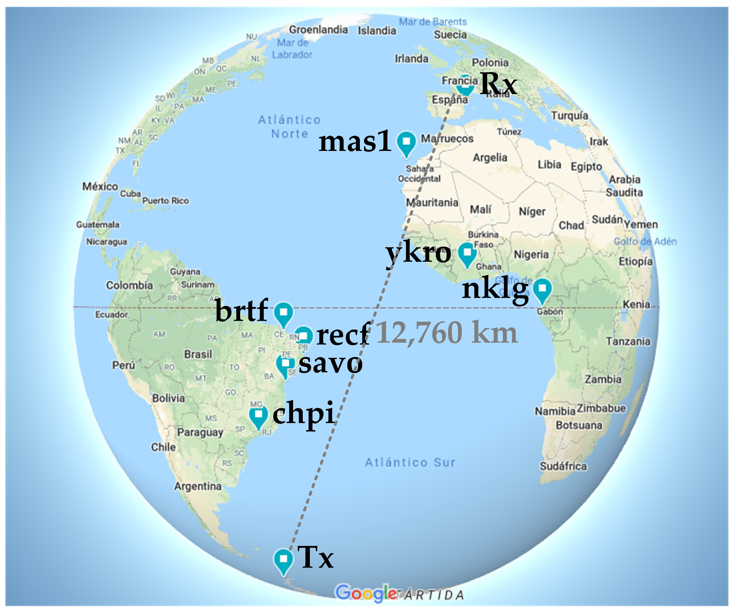
Variation of Ionospheric Narrowband and Wideband Performance for a 12,760 km Transequatorial Link and Its Dependence on Solar and Ionospheric Activity

Abstract

The ionosphere provides a channel that is able to propagate electromagnetic waves for long-haul communications, allowing Non-Line-Of-Sight (NLOS) radio communications in the high-frequency band (HF). Nonetheless, its performance as a communications channel mainly depends on solar activity, as Earth’s diurnal and seasonal cycles modify the ionospheric ionization by the sun and consequently the channel performance. La Salle and the Observatori de l’Ebre have conducted oblique soundings of a 12,760 km ionospheric channel from Livingston Island (South Shetland Archipelago—Antarctica $-{62.7}^{\circ }$S, ${299.6}^{\circ }$E) to Cambrils (Spain $-{41.0}^{\circ }$N, ${1.0}^{\circ }$E) to evaluate this evidence and analyze the characteristics of this particular channel. The final goal of the project is to establish a stable communications link to be used as a backup for low throughput data transmission from the various geomagnetic and meteorological sensors located in the Spanish Antarctic Station. The aim of this paper is to confirm the relationship between the channel availability of narrowband and wideband communications and the resulting channel parameters with the solar and ionospheric activity for four consecutive sounding campaigns.

1. Introduction

The ionosphere is a hostile channel for high-frequency (HF) radio communications due to the several phenomena that constantly change the its performance conditions. The ionization varies considerably depending on the activity of the Sun, and the variations of the solar flux radiation, such as ultraviolet and X-ray radiation, can have significant effects [1]. An awareness of this variation becomes absolutely central when attempting to model a given ionospheric channel for communication purposes [2]. The variations of solar activity, which are mainly dominated by the solar cycle (which lasts for approximately 11 years) and solar rotation (27 days), are not the sole cause of ionospheric variability; seasonal and diurnal variations—and even variations with a shorter time scale—play a significant role in ionospheric variability [3]. A summary of these variations is discussed in [4], considering durations from short-term variations (e.g., traveling ionsopheric disturbances) to long-term changes (e.g., solar cycle), while [5,6] have focused on the planetary and gravity-wave signatures in the F-region ionosphere (variations with periods shorter than 18 days) which can impact radio propagation predictions and variability. At low latitudes, disturbances related to equatorial plasma bubbles (EPBs) contribute significantly to the ionospheric variability [7]. Such disturbances are closely related to the well-known Equatorial Spread-F phenomena [8] (ESF) which are consequences of the diffusive nature of the ionospheric echoes produced by radio scattering from electron density irregularities [9].

La Salle and the Observatori de l’Ebre teams have been sounding the 12,760 km ionospheric channel from Livingston Island in the South Shetland Archipelago (${62.7}^{\circ }$S, ${299.6}^{\circ }$E) to Cambrils (${41.0}^{\circ }$N, ${1.0}^{\circ }$E) for 11 years [10] (see Figure 1); from the first soundings, several hops were estimated [11] to save this transequatorial link. Our team has deployed and set in operation an oblique ionosonde in the Spanish Antarctic Station (SAS) on Livingston Island every austral summer in order to conduct experiments. The transmitting antenna of the sounder was a 7.5 m rugged monopole fed by only 250 W for environmental reasons and the power restrictions of the SAS. The transmitted radio wave was received in Cambrils (Spain) using the aforementioned monopole and an inverted V antenna (see Figure 2).

There is a clear relation between the successful transmission frequencies and solar activity as estimated by the the well-known Sun spot number (SSN) [12] parameter, which clearly shows the solar variation and cycles [13,14]. The relations between radio propagation and Sun phenomena have been widely studied in the past [15]. Narrowband sounding was already presented in [16], and tests of the dependence of its availability on solar activity were conducted in several studies. These studies have led us to conclude that narrowband propagation has a strong dependence on solar activity variations due to its influence on ionospheric performance in terms of electromagnetic propagation. The results obtained through these campaigns show that the higher the SSN, the better the performance of the ionospheric channel for narrowband communication. This paper presents the study of the variation of the propagation availability of the 12,760 km ionospheric radio link for wideband communications. The study analyzes the four campaigns with available wideband soundings with the aim of determining the dependence of the propagation availability on solar activity for wideband sounding. Moreover, this trans-equatorial radio-link allows us to study the potential effects of ionospheric irregularities on wideband sounding. The results are based on the analysis of all the wideband sounding parameters (e.g., Doppler spread, delay spread, number of paths and signal-to-noise ratio).

This paper is organized as follows: Section 2 details the sounding system used to conduct the measurements. Section 3 presents the narrowband and wideband sounding methodology, and Section 4 details the results of the wideband soundings, their dependence on the SSN and the potential effects caused by ionospheric irregularities. Section 5 presents the conclusions.

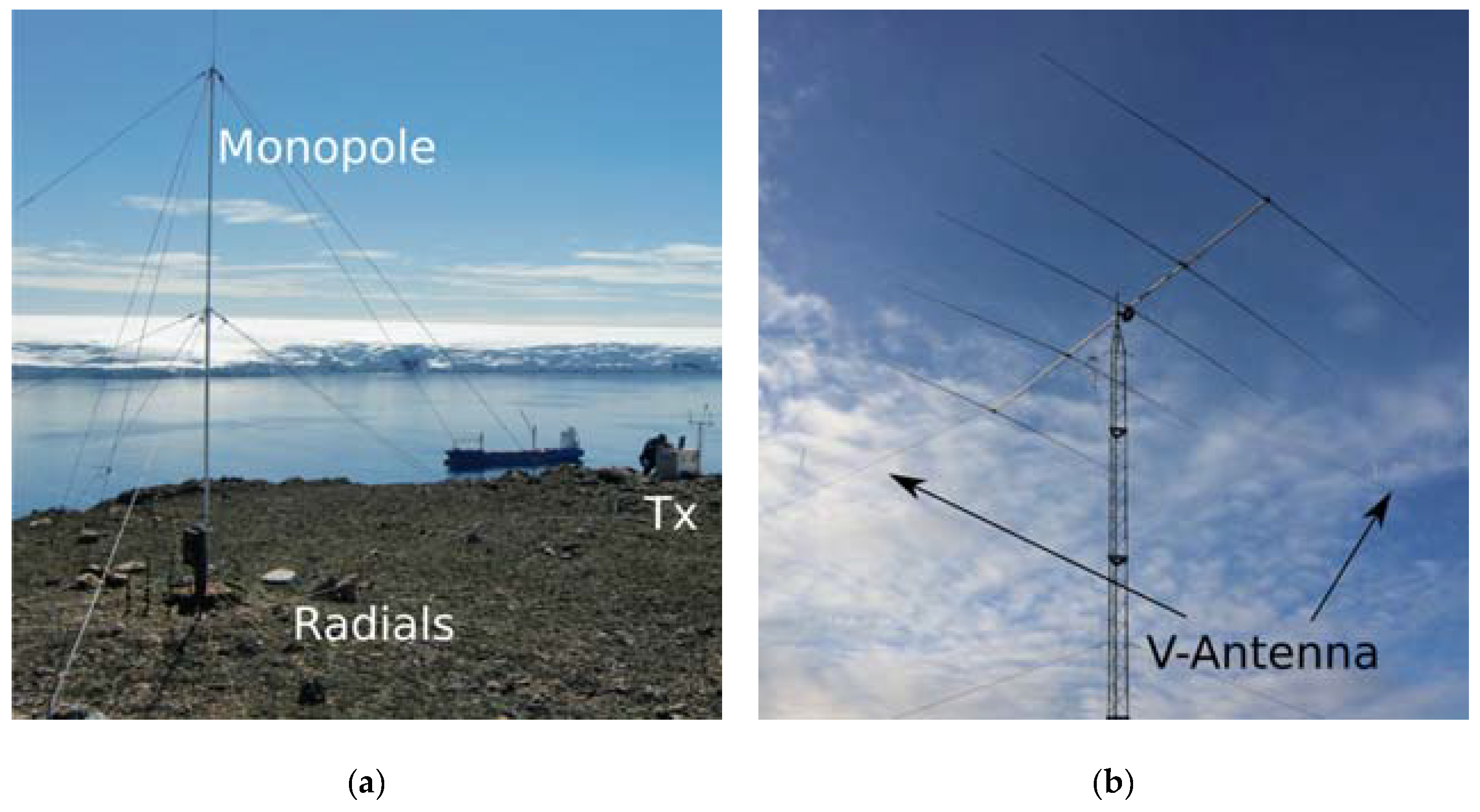
2. System Hardware Description

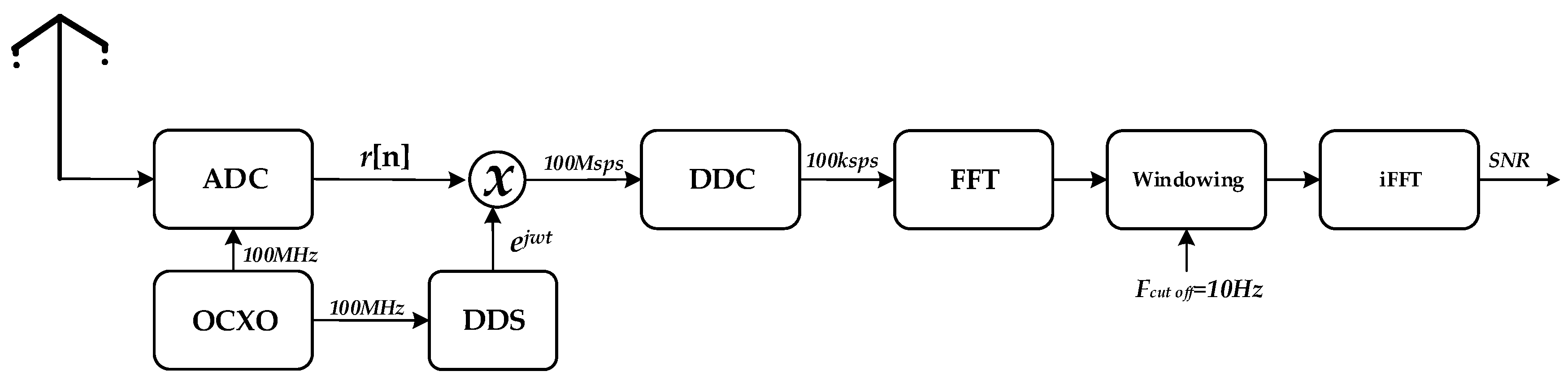
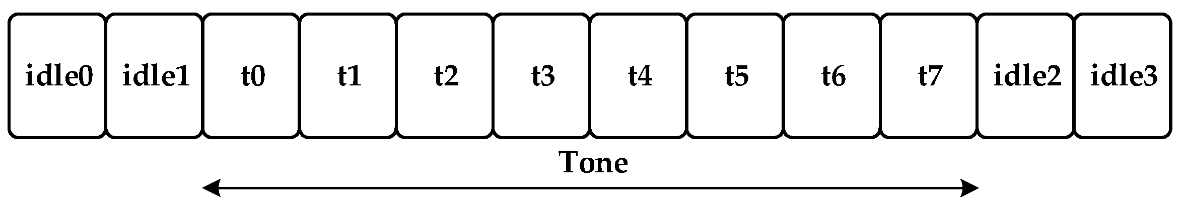
The oblique incidence ionospheric sounder has been in operation since 2003 [17]. This allows the channel to be analyzed by means of narrowband and wideband soundings. The system was upgraded during the Antarctic survey 2009–2010, and the results of the analysis of the improvements to the transmitter and receiver were presented in [18]. Thanks to the last system upgrade, it was possible to overcome some of the limitations of the former system described in [11]. The new system can work (i) in a larger frequency range (2 to 30 MHz) and for 24 h a day; (ii) with a higher accuracy of frequency synchronization, using an oven controlled crystal oscillator (OCXO); (iii) with better time accuracy (1 $\mathsf{\mu }$s) thanks to a new GPS; and finally (iv) with high-speed analog-to-digital and digital-to-analog converters (ADC and DAC, respectively) [19].

The antenna used in the transmitter (Tx) is a 7.5 m rugged monopole, with an antenna tuner that can adapt the whole HF band [20] (see Figure 2a). The Tx antenna was located at the top of a small hill on Livingston Island, close to the SAS, with a clear view of the receiver and 32 radials of 15 m in length and 2.5 mm${}^2$ sections were used to improve the gain in the middle frequencies by 2 dB (around 15 MHz). We deployed two different receiver antennas (Rx) in the receiving site, in a clear grassland in Cambrils: a 7.5 m rugged monopole (picture not available, but it is a replica of the transmitter antenna) and an inverted V antenna (see Figure 2b; the thin wires indicated by the arrows).

However, the results presented in this work only use the data collected by the inverted V antenna, which does not need a tuner to work at any frequency. The transmission power is limited to 250 W due to SAS restrictions. The reader is referred to [18,21] for more details.

3. Channel Sounding

The sounding of a communication channel is carried out both in narrowband and in wideband to cover all possible scenarios in a communication system [22]. On the one hand, narrowband sounding focuses on channel availability and the signal-to-noise ratio (SNR) [11] and is a good metric to use to determine when there are fadings in the channel; on the other hand, wideband sounding [10] is conducted by means of pseudonoise sequences [23], which lead by means of correlation in the receiver to the impulse response of the channel to define the time-variation of the ionospheric propagation. The impulse response of the channel is used to compute the scattering function, and this in turn is used to evaluate the multipath delay spread and Doppler spread, and even to count the number of received paths. All of the parameters (availability, SNR, multipath delay spread, Doppler spread) are key issues for the determination of the channel variations in terms of propagation over time and represent the base on which a physical layer for any communications system can be built [21].

3.1. Narrowband Metrics

The narrowband sounding analysis is focused on SNR and channel availability computation from the received data (see Figure 3). The channel availability is defined as the probability of a communication link reaching a minimum SNR value and therefore achieving a certain quality of service (see [24] for more details). A minimum value of SNR must be set to conduct channel impulse response estimation; in this situation, we follow the proposal of Vilella [11], who specifies a minimum SNR of 6 dB using a 10 Hz bandwidth.

The evaluation of the SNR is conducted using the following method. In the receiver, the signal is sampled at 100 Msps, downconverted into a baseband signal and downsampled to 100 kilo-samples per second (ksps). The fast Fourier transform (FFT) [25] is used, and the results are low-pass filtered with a 10 Hz Kaiser window [26] to reduce high frequency components.

As the metrics evaluated for SNR can be easily distorted due to interference, a time framing technique is used, consisting of dividing the tone slot into eight smaller subslots of 1 s each and evaluating the evolution of the SNR for the entire slot (see Figure 4). The SNR is computed for each 1 s slot by means of the ratio of the power of every signal slot over the power of each noise slot according to the following:

$$SN{R}_{ij}=\frac{S_i+N_i}{N_j},$$

(1)

where $S_i$ and $N_i$ show the power of the desired signal and noise, respectively, at slot i, and $N_j$ is the noise power at slot j. The entire SNR is then evaluated as

$$SNR=\frac{1}{KL}\sum _{j=1}^K\sum _{i=1}^{L}SN{R}_{ij},$$

(2)

assuming that L is number of signal slots and K is the number of noise slots.

3.2. Wideband Metrics

In this section, we present an analysis of the variation of the Doppler spread and the delay spread, as well as of the number of paths, which will give us more detail about the potential influence of the variations of solar activity. The multipath spread or the delay spread is a measure of the richness of the multipath component in a communication; it can be interpreted as the difference between the arrival of the earliest significant signal and the arrival of the latest multipath component [27]. The Doppler spread is the difference between the Doppler shifts of the different components that contribute to a signal fading tap in the channel, and the Doppler shift is the slight frequency change of the signal transmitted along each path in a communication [27].

Wideband sounding measurements have been carried out for all frequencies ranging from 2 to 30 MHz at a 500 kHz sampling rate. Therefore, 57 different frequencies have been analyzed every hour, resulting in a total of 1368 daily measurements. The details of the wideband sounding are as follows: (i) a sampling frequency of 100 ksps, (ii) a pseudo noise (PN) m-sequence length [23] of 255 chips, (iii) a chip frequency of 5 kHz and (iv) 200 PN sequences per test.

Figure 5 indicates the computational process for the wideband sounding. The wideband analysis is crucial to the characterization of the time and frequency dispersion in the channel.

First, the received signal $r\left[n\right]$ is correlated with the original PN m-sequence to obtain the channel impulse response in the time domain:

$$h[n,\tau ]={\varphi }_{r,S_e}[nl{N}_c+\tau ]$$

(3)

where $\tau$ is the delay variable, l is the number of chips, $N_c$ is the number of samples per chip and $S_e$ is the PN m-sequence. The scattering function $R_s[\tau ,v]$ is obtained as the discrete Fourier transform (DFT) of the channel impulse response [27]:

$$R_h[\xi ,\tau ]=\sum _{\xi }{h}^{*}[n,\tau ]h[n+\xi ,\tau ]$$

(4)

$$R_s[\tau ,v]=\sum _{\xi }{R}_h[\xi ,\tau ]e^{-j2\pi \xi v}$$

(5)

Both the composite multipath spread and the composite Doppler spread are calculated from the data obtained in the scattering function $R_s[\tau ,v]$]. Let $[{\tau }_1,{\tau }_2]$ be the multipath observation window and $[v_1,v_2]$ the Doppler spread observation window; consequently, both the multipath and the Doppler power profiles are defined by

$$\varphi \left[\tau \right]=\sum _{v=v_1}^{v_2}{R}_s[\tau ,v]$$

(6)

and

$$\varphi \left[v\right]=\sum _{\tau ={\tau }_1}^{{\tau }_2}{R}_s[\tau ,v]$$

(7)

Given the maximum delay and Doppler spread values obtained in previous tests [11], we have analyzed only the received signals with delay and Doppler spread measures within the [−3.5, 3.5] ms and [−2.5, 2.5] Hz ranges, respectively. Afterwards, we calculated the spread parameters. The multipath spread is measured from the multipath power profile as 80% of the power spread [11]; this measure is named the composite multipath spread $\left(t_{eff}\right)$ and was defined in [15]. Similarly, the Doppler spread is measured from the Doppler power profile as the 80% power spread; this measure is named the composite Doppler spread $\left(u_{eff}\right)$ and was defined in [28].

Finally, the last of the wideband analyses is the number of paths, which is defined as follows. The number of paths is obtained by evaluating the number of peaks found at the energy thresholds of 70% and 45% that correspond to the strongest path (the maximum value); the system assumes that the number of paths is the largest value obtained, because not all the paths are properly separated. The two thresholds were set by testing the results over the data, measuring which levels of energy were more suitable to determine the real number of paths for each type of response.

4. Results

In this section, we present the different results obtained of the narrowband (availability) and wideband soundings (delay, Doppler and number of paths) for different campaigns conducted under different solar activity levels, as indicated by SSN values [29]. We also show the differences in the performance of the soundings when ionospheric disturbances occur near to the path of the radio-link, compared to a time in which no disturbances happen.

Table 1. Details of the four studied campaigns. SSN: Sun spot number.

Survey	Start Date	End B	# Days	# Total Files	# Avail. Files (%) Files	Avail.	Averaged SSN
2010/2011	22/1/2011	1/3/2011	39	53,352	2719	5.1	42
2011/2012	13/2/2012	25/2/2012	13	17,784	2476	13.92	56
2012/2013	5/1/2013	24/02/2013	51	69,768	17,268	24.75	78
2013/2014	24/1/2014	18/2/2014	26	35,568	17,729	49.85	123

indicates the start and end date for the four sounding campaigns analyzed, as well as the number of working days of the system. Campaign 2010–2011 coincided with low solar activity, and this will probably be reflected in the propagation results; Campaign 2011—2012 was short due to logistic issues, and only a few days of measurements were possible, resulting in poor statistical results.

Most of the data received during the four campaigns show no available channel for communication [16], so there is a low number of measurements with data available to study. This resulted in a short number of files to study (see Table 1). Although the total number of measurements that recorded usable data (40,192) versus the total number of measurements carried out for the four campaigns (176,472) is a relatively small percentage (23%), it is considered reasonable in this exhaustive sounding.

Table 1 shows the mean value of the SSN for each of the surveys as an estimate of the average solar activity when the measurements were carried out.

4.1. Aggregated Results Depending on Solar Activity

Figure 6 shows the aggregated results of availability, composite delay spread, composite Doppler spread and the number of paths of the four campaigns with a box-and-whisker plot [30]. This range-bar draws a box to display a group of metrics in a standardized manner, with a middle line in red that stands for the median of the data aggregated in each of the box-and-whisker plots. The upper part of the box is the limit between the first and second quartile. The lower part of the box is the limit between the third and the fourth quartile. Finally, the individual points show the outliers.

Figure 6a compares the percentage availability in the different campaigns and shows that the best campaign was that of 2013–14, which coincided with the largest solar activity (Table 1). Campaigns 2011–12 and 2012–13, carried out under similar solar activity, but which was lower than that of 2013–14, showed lower availability values than those measured for Campaign 2013–14. Finally, Campaign 2010–11 showed the lowest availability of the four surveys under study, and the solar activity was also the lowest.

The composite delay spread (Figure 6b) and composite Doppler spread (Figure 6c) show similar behaviors to the reported results of percentage availability. The highest delay and Doppler spread with mean values close to 2 ms and 0.5 Hz, respectively, correspond to Campaign 2013–14, when the solar activity was the greatest (Table 1). However, the lowest delay and Doppler spread, with mean values close to 1 ms and 0.1 Hz, respectively, were found for Campaign 2010–11, when the lowest solar activity was observed. Note that Campaigns 2011–12 and 2012–13 showed mean values of delay and Doppler spread within those reported for Campaigns 2010–11 and 2013–14, while the SSNs for Campaigns 2011–12 and 2012–13 also showed values between those measured for Campaigns 2010–11 and 2013–14. All campaigns except Campaign 2013–14 showed a Doppler median value of 0.25 Hz or lower and had three quartiles below 0.5 Hz. Campaign 2013–14 showed slightly higher values in the Figure 6c, with a median Doppler value close to 0.5 Hz with the measures of three quartiles below 0.75 Hz.

Therefore, there appears to be a positive trend in terms of the percentage increase in availability, delay spread and Doppler spread with increasing solar activity. The mean value of the delay spread for Campaign 2011–12 was slightly greater than expected, but we must take into account the few days of possible measurements for that survey. Finally, the behavior of the number of paths gives no clear trend with respect to solar activity (Figure 6d). Campaigns 2011–12 and 2012–13 showed median values of approximately 2.5 detected paths, whereas Campaigns 2013–14 and 2010–11 showed slightly lower median values, with about two paths being detected. Despite this slight difference, the number of paths in the four campaigns remained uniform and was not substantially modified by the solar activity. This box-and-whisker plots show some situations with a higher number of paths—even more than 10 paths—which can arise from error measurements due either to noise or the low signal-to-noise ratio (SNR) channel, where the calculation of the number of paths is not sufficiently accurate.

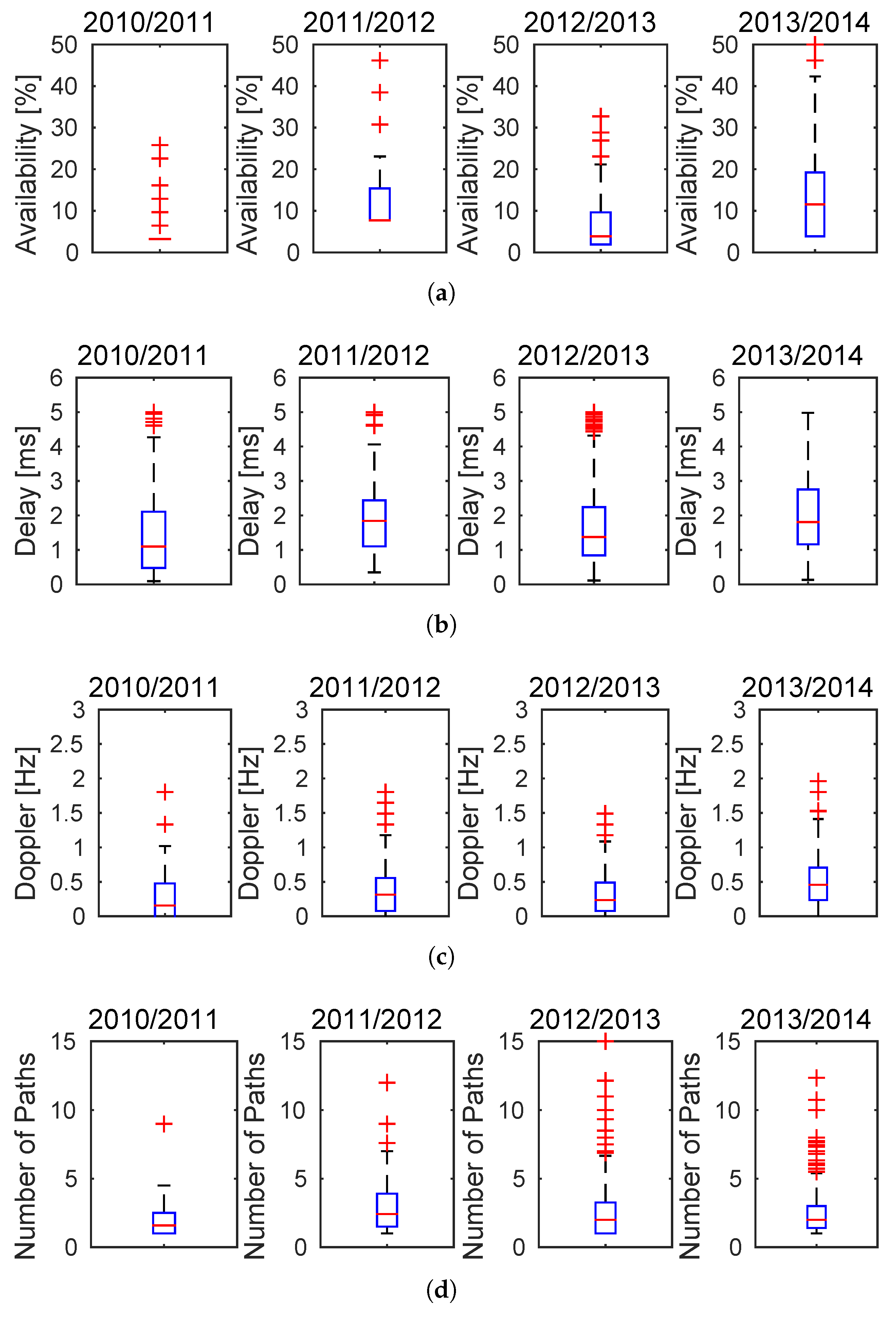
4.2. Delay, Doppler and Number of Paths Per Campaign

This section reports on the distribution of the delay and Doppler spread and number of paths estimated for the oblique sounding as a function of the frequency and of the time of the day. Figure 7 depicts the three measurements for the four campaigns, and the following observations can be highlighted.

Campaign 2011–12 had few available files, and most of the measurements carried out in Campaigns 2010–11 and 2011–12 resulted in a low number of representative results for the available frequencies and times. Despite this fact, there is a similarity between the trend of the solar activity (average SSN) and the trend of the number of successful oblique sounding measurements: the greater the solar activity, the higher the successful soundings. Note that Campaign 2013–14 was short in terms of its number of days compared to Campaigns 2010–11 and 2012–13, but the number of successful propagation measurements was very good in the campaign, which was probably related to the high solar activity. However, the results are similar for all four campaigns if we compare the daily pattern and frequency dependence of the composite delay spread, composite Doppler spread and the number of paths. The composite delay spread (Figure 7a,d,g,j) indicated lower values—a maximum of 1.5 ms— from 08 UTC to 19 UTC and at high frequencies (above 16 MHz), and from 20 UTC to 07 UTC for frequencies above 13 MHz when propagation was possible.

Note that values which are larger than 5 ms of composite delay spread are not drawn in these four figures, given the fact that they are unlikely to appear. Higher values of composite delay spread—a maximum of 3–3.5 ms—were found starting at 20 UTC and at maximum frequencies of 10–12 MHz. Results concerning the composite Doppler spread (Figure 7b,e,h,k) showed lower values from 08 UTC to 19 UTC and especially at high frequencies, and higher Doppler values were recorded from 20 UTC to 07 UTC, usually with maximum values of about 0.6 to 0.8 Hz. The behavior of the composite Doppler spread differed between day and night, but not as clearly as the composite delay spread. Finally, the number of paths (Figure 7c,f,i,l) of the oblique sounding showed smaller mean values of number of paths during the daytime (8-19 UTC), with a maximum value of about two paths, compared to nighttime (20-7 UTC), when high values were collected—especially at lower frequencies—sometimes indicating that three and four paths were possible at the receiver. The changes in the number of paths between different campaigns were not substantial, indicating a low effect of solar activity on the number of paths.

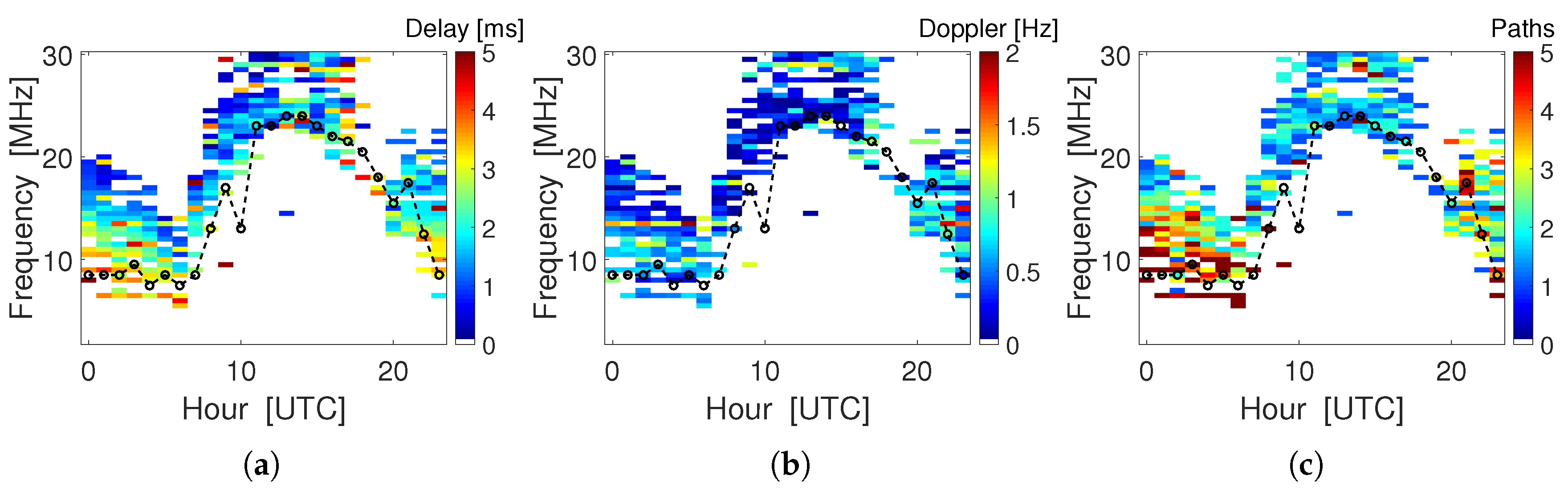
4.3. Delay, Doppler and Number of Paths vs Narrowband FLA

We also present the comparison between characteristics of narrowband and wideband soundings; Figure 8 depicts the frequency with largest availability (FLA) measured over the narrowband signal [16] with the matrices showing the results for the composite delay spread, the composite Doppler spread and the number of paths for Campaign 2013–14.

The availability of the channel in wideband sounding has been evaluated with different considerations to those of the narrowband soundings, as explained in Section 3. However, most frequency values chosen for their good propagation in narrowband also show good performance in wideband. The few exceptions to this are probably due to ionospheric instability during the measurements. Figure 8 shows that the FLA of the narrowband sounding for nighttime corresponds to frequencies with higher values of the composite delay spread, of the composite Doppler spread and of the number of paths. The opposite is shown during the daytime, when the FLA in narrowband coincides with frequencies showing lower values of the composite delay spread, of the composite Doppler spread and of the number of paths.

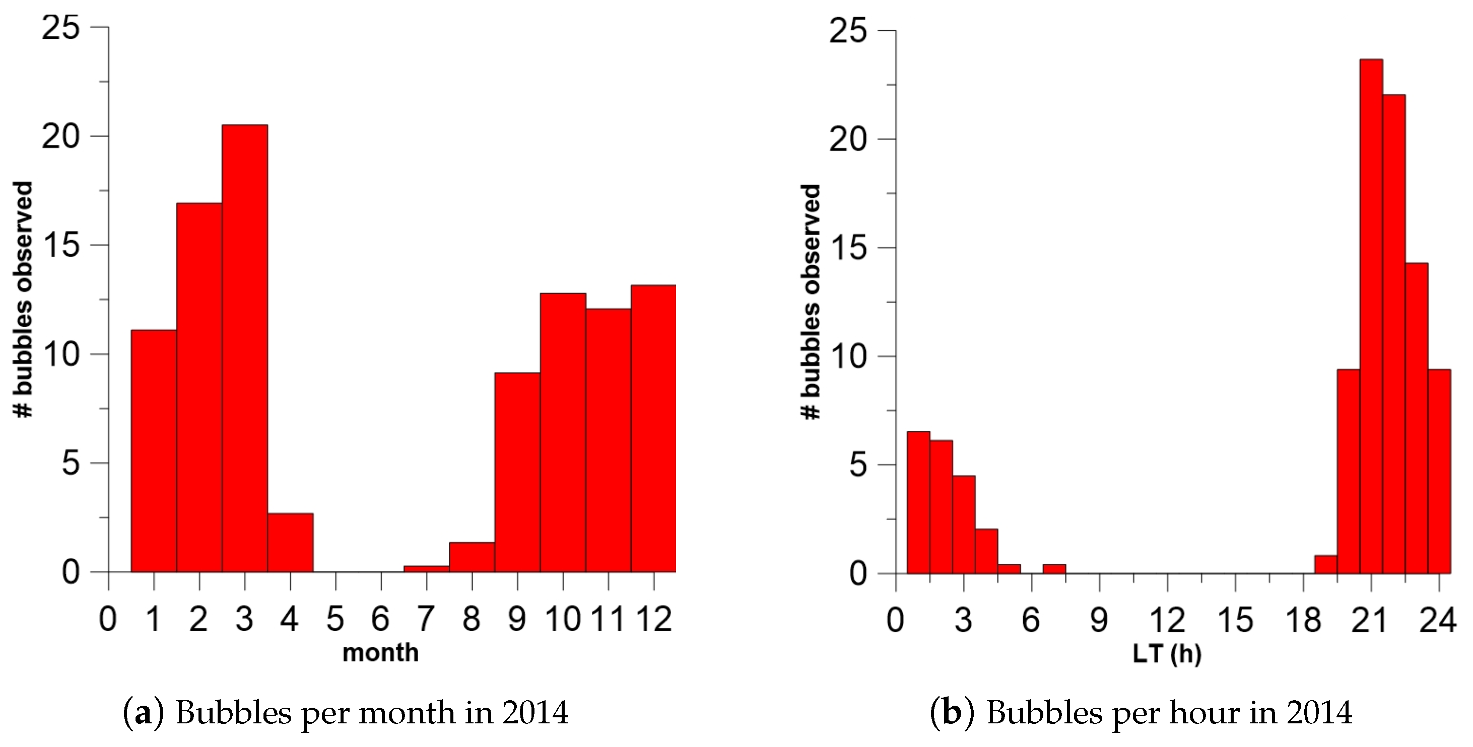
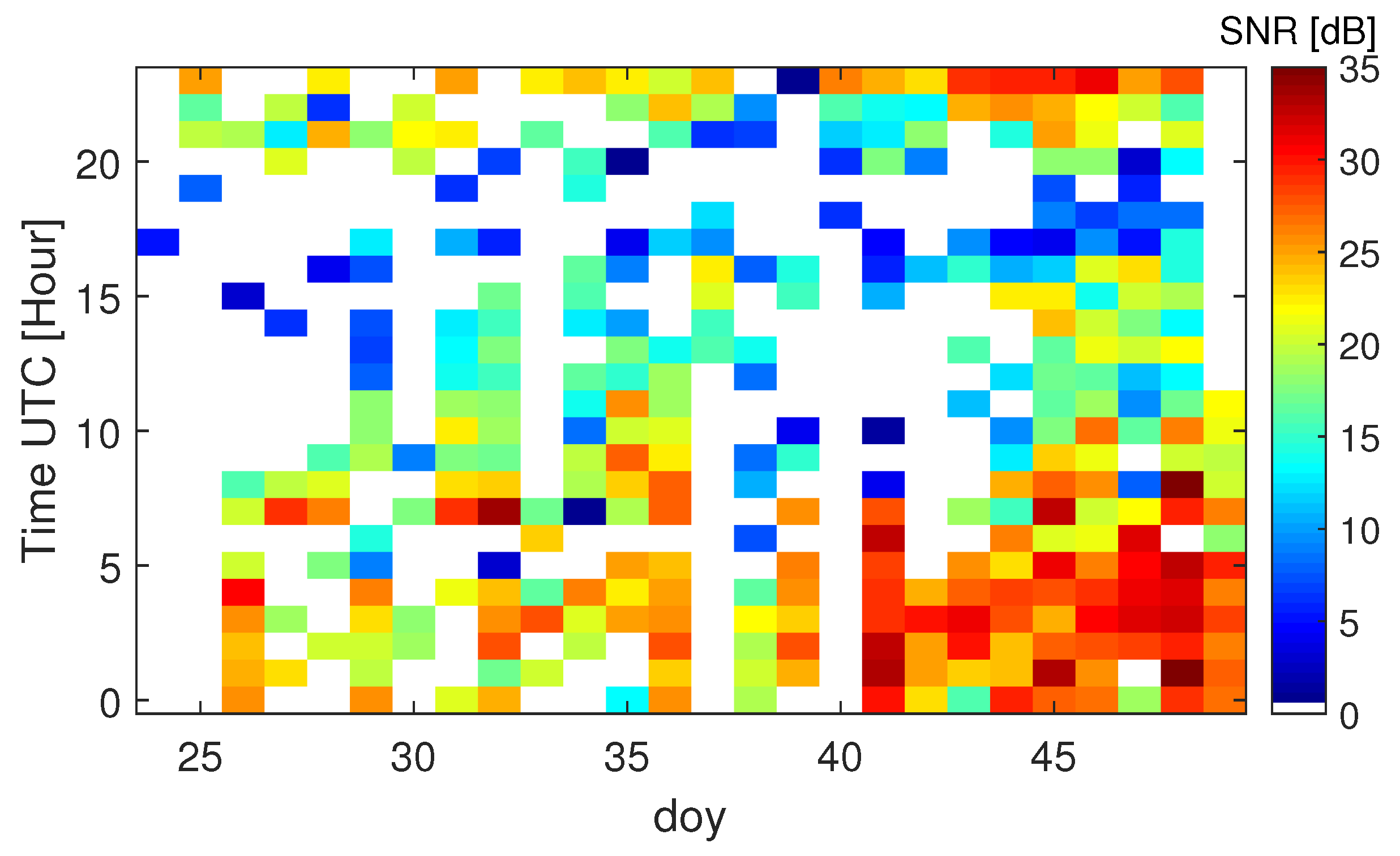
4.4. Effects of Ionospheric Irregularities on Wideband Sounding

The current ionospheric sounding for such a trans-equatorial radio might be affected by the ionospheric irregularities developed through line-of-sight. At low latitudes, the ionosphere leads to the well-known equatorial plasma bubbles (EPBs) phenomenon, which are plasma density depletions that occur after sunset and develop during the night in the equatorial region [7]. Just after sunset, the equatorial ionosphere experiences an east–west electric field, which in conjunction with the north-south magnetic field causes the ionospheric plasma to drift upward [31]. This effect, added to the recombination of molecular species at the nighttime bottomside F region, causes an apparent upward movement of the equatorial F layer [32]. The occurrence probability of the EPB correlates with the vertical plasma drift, enhanced just after sunset and with solar activity; i.e., the higher the solar activity, the higher the occurrence probability [33]. Moreover, statistical studies have shown that the highest probability of EPB occurs in the equinoctial season and slightly shifts towards December and February in the Brazilian longitudinal sector; furthermore, it has been shown that the duration of EPBs can exceed one hour [34].

We have applied the method described in [34] to the data from several receivers of the Global Navigation Satellite System (GNSS) to search for potential irregularities that might affect wideband sounding. The analyzed receivers were selected as they were sufficiently close to the path of the transequatorial radio-link (Figure 1) and belong to the International GNSS Service (IGS) network. These data are available from the Crustal Dynamics Data Information System Data Center, ftp://cddis.gsfc.nasa.gov/pub/gps/data/daily/. The method was inspired by the work presented in [33], and the detection of plasma depletions was improved by analyzing the second difference of the total electron content (TEC) estimated by the geometry-free combination of the ground-based GNSS carrier phase delays ($LI=L1-L2$) instead of the first difference of the slant TEC (sTEC). This allows us, on one hand, to analyze a larger amount of data, because using TEC instead of sTEC means that there is no need to apply an elevation mask when using LI to avoid the effects of low-elevation data, and on the other hand, this also allows a better determination of the initial and final time of the perturbation, because the second derivative of TEC is less noisy than the first derivative. In addition, the method described in [34] introduces the use of the noisier but unambiguous code ($PI=P1-P2$) to reconstruct the TEC perturbation when phase ($LI=L1-L2$) is not available due to cycle slips or a loss of lock, which makes it possible to increase the amount of analyzed data and to detect large perturbations that could not be detected by LI. The method detects the disturbances over GNSS stations and provides information about the location, duration and depth of the plasma depletion caused by EPBs. As an example, Figure 9 depicts the seasonal and daily occurrence of EPBs above the mas1 station in the Canary Islands for the year 2014. The results shown in Figure 9 indicate that EPBs over mas1 tend to occur mostly after sunset and during winter seasons.

EPBs cause specific signatures in the propagation of radio signals as scintillations in the very high-frequency band (VHF) and frequency and range spread in the equatorial ionograms [35]. Therefore, the observed increase of the composite delay spread in nighttime (Figure 7a,d) cizkd be an effect of the activity of EPB, which can create extra ionogram reflections or a spreading of the layer reflection as a consequence of additional oblique reflection in the walls of the EPB. The latter fact in combination with the daily occurrence of EPBs can explain the observed larger delay spread for nighttime; moreover, the occurrence of EPBs and the enhanced electrodynamics of the low latitude and equatorial ionosphere during nighttime can explain the observed larger composite Doppler spread and the increased number of paths during nighttime compared to daytime.

We have studied the variations of the SNR of the wideband soundings to evaluate the potential effects of the ionospheric irregularities on the channel performance. For a given day and at a given time, we have selected the frequencies of transmission that report the largest SNR at the receiver. Figure 10 shows the results of the aforementioned SNR for Campaign 2013–14. Figure 10 shows that the SNR presents lower values at the time near to sunset (1800–1900), coinciding with the enhancements of the vertical plasma drift at low latitudes [33], the occurrence of EPBs [34] and the ESF [8]. Note that zero values of SNR in Figure 10 (white values) mean that there are no reliable observations due to either technical problems with the transmitter or a very low SNR, with a channel availability less than 5% of the time. As already pointed out earlier, EPBs can produce radio scattering and a diffusive nature of the ionospheric echoes [9]. Moreover, F-scatter propagation can result in a weakening signal by 30 to 40 dB, which is attributable to diffraction effects [36]. Figure 10 also shows that the SNR is significantly higher (by a factor of 1.25) for day of year (doy) 40 and later compared to the previous days of the campaign, especially from 2200 to 0700.

Figure 11 shows the activity of EPBs as observed in the low-latitude ionosphere at the east coast of Brazil. The results depicted in the Figure 11 indicate that the activity of occurrence of EPBs at this site is significantly lower (by factor 2) for day of year (doy) 40 and later compared to the previous days of the campaign. Although not shown, other stations report similar results to those reported for Savo station in Brazil, indicating that the EPB activity recorded in the Atlantic sector is significantly lower for doy 40 and later compared to the previous days of the campaign.

It must be noted that EPB activity is mainly observed for the local time sector after sunset (e.g., Figure 9b). The dominant occurrence of EPB activity after sunset (Figure 9b) and the observations of increased EPB activity for days of year (doy) 24 to 39 (Figure 11) coincide with observations of the low SNR of the signal of the trans-equatorial radio-link (Figure 10). However, we observe low EPB activity for doys 40 to 49 of the campaign (Figure 11), which coincides with the large SNR observations of the signal of the trans-equatorial radio-link (Figure 10) compared to previous days. According to [9], EPBs can produce radio scattering and the diffusive nature of the ionospheric echoes, and F-scatter propagation can result in a weakening signal by 30 to 40 dB, which is attributable to diffraction effects [36]. The later agrees with results reported in Figure 10 and Figure 11. The dominant SNR measurements for doys 23 to 39 at night (2200–0700), when the EPB activity is large, are about 22–24 dB, whereas the dominant SNR measurements for doys 40 to 49, when EPS activity is low, are about 30–32 dB. Therefore, comparing the results of Figure 10 and Figure 11, we propose that the higher activity of EPBs can explain the measurements with lower SNRs, or vice-versa, the low SNRs recorded for a given time interval might indicate an enhanced occurrence of ionospheric irregularities through the path of a particular trans-equatorial radio-link.

5. Conclusions

This paper studies the potential relationship between solar activity (SSN) and the propagation of a wideband signal in a 12,760 km long haul ionospheric link between Antarctica and Spain. We conclude from the study that the higher the solar activity, the higher the mean value of the composite delay spread and the composite Doppler spread; however, no significant influence of solar activity is observed in terms of the number of paths in the propagation. Certainly, the data campaigns analyzed are not completely sufficient to allow us to conclude with certainty that both composite delay spread and composite Doppler spread are larger when the solar activity is greater: nevertheless, it is a fact that greater solar activity corresponds to larger ionospheric ionization, which in turn allow larger frequency ranges to be available for radio-sounding measurements. In addition, the activity of ionospheric irregularities such as EPBs increases as the solar activity increases. We can also conclude that a higher composite delay and Doppler spread and a higher number of paths occur during nighttime propagation, and the lower values for the three conducted measurements correspond to daytime propagation in higher frequencies.

The significant similarities between the occurrence of the EPBs and enhanced electrodynamics of the low latitude and equatorial ionosphere for nighttime, alongside the observed higher values of the composite delay spread, of the composite Doppler spread and of the increased number of paths observed for this trans-equatorial radio link, indicate that changes in wideband sounding performance could be used as a sensor to estimate equatorial ionospheric irregularities. Moreover, detailed inspection of the day-to-day variation of the occurrence of EPBs and of the recorded SNR or the trans-equatorial radio-link would also support the potential use of such a sensor as an estimator of equatorial ionospheric irregularities. Finally, we can conclude that the frequency with the largest availability evaluated in narrowband using the signal-to-noise ratio criteria mostly coincides with higher propagation success in wideband tests.

References

1. Rishbeth, H.; Garriott, O.K. Introduction to Ionospheric Physics; Academic Press: New York, NY, USA, 1969. [Google Scholar]
2. Angling, M.; Shaw, J.; Shukla, A.; Cannon, P. Development of an HF selection tool based on the Electron Density Assimilative Model near-real-time ionosphere. Radio Sci. 2009, 44. [Google Scholar] [CrossRef]
3. Forbes, J.M.; Palo, S.E.; Zhang, X. Variability of the ionosphere. J. Atmos. Sol. Terr. Phys. 2000, 62, 685–693. [Google Scholar] [CrossRef]
4. Rishbeth, H.; Mendillo, M. Patterns of F2-layer variability. J. Atmos. Sol. Terr. Phys. 2001, 63, 1661–1680. [Google Scholar] [CrossRef]
5. Altadill, D.; Apostolov, E. Time and scale size of planetary wave signatures in the ionospheric F region: Role of the geomagnetic activity and mesosphere/lower thermosphere winds. J. Geophys. Res. 2003, 108. [Google Scholar] [CrossRef] [Green Version]
6. Altadill, D.; Apostolov, E.M.; Boska, J.; Lastovicka, J.; Sauli, P. Planetary and gravity wave signatures in the F-region ionosphere with impacton radio propagation predictionsand variability. Ann. Geophys. 2004, 47, n.2/3. [Google Scholar]
7. Huang, C.S.; de La Beaujardiere, O.; Roddy, P.A.; Hunton, D.E.; Liu, J.Y.; Chen, S.P. Occurrence probability and amplitude of equatorial ionospheric irregularities associated with plasma bubbles during low and moderate solar activities (2008–2012). J. Geophys. Res. 2014, 119, 1186–1199. [Google Scholar] [CrossRef]
8. Woodman, R. Spread F—An old equatorial aeronomy problem finally resolved? In Annales Geophysicae; Copernicus GmbH: Göttingen, Germany, 2009; Volume 27, pp. 1915–1934. [Google Scholar]
9. Booker, H.; Wells, H. Scattering of radio waves by the F-region of the ionosphere. Terr. Magn. Atmos. Electr. 1938, 43, 249–256. [Google Scholar] [CrossRef]
10. Hervás, M.; Alsina-Pagès, R.M.; Orga, F.; Altadill, D.; Pijoan, J.L.; Badia, D. Narrowband and wideband channel sounding of an Antarctica to Spain ionospheric radio link. Remote Sens. 2015, 7, 11712–11730. [Google Scholar] [CrossRef] [Green Version]
11. Vilella, C.; Miralles, D.; Pijoan, J. An Antarctica-to-Spain HF ionospheric radio link: Sounding results. Radio Sci. 2008, 43, 1–17. [Google Scholar] [CrossRef]
12. Ostrow, S.; PoKempner, M. The differences in the relationship between ionospheric critical frequencies and sunspot number for different sunspot cycles. J. Geophys. Res. 1952, 57, 473–480. [Google Scholar] [CrossRef]
13. Clette, F. Sunspot Index and Long-Term Solar Observations. Available online: http://www.sidc.be/silso/home (accessed on 2 May 2019).
14. Clette, F.; Cliver, E.; Lefèvre, L.; Svalgaard, L.; Vaquero, J. Revision of the sunspot number (s). Adv. Space Res. 2015, 13, 529–530. [Google Scholar] [CrossRef] [Green Version]
15. Angling, M.J.; Davies, N.C. An assessment of a new ionospheric channel model driven by measurements of multipath and Doppler spread. In Proceedings of the IEE Colloquium on Frequency Selection and Management Techniques for HF Communications, London, UK, 29–30 March 1999; pp. 4/1–4/6. [Google Scholar] [CrossRef]
16. Orga, F.; Altadill, D.; Hervás, M.; Alsina-Pagès, R.M. Interannual Variation of a 12,760 km Transequatorial Ionospheric Channel Availability and Its Dependence on Ionization. In Proceedings of the 1st International Electronic Conference on Atmospheric Sciences (ECAS 2016), Basel, Switzerland, 16–31 July 2016. [Google Scholar]
17. Pijoan, J.L.; Altadill, D.; Torta, J.M.; Alsina-Pagès, R.M.; Marsal, S.; Badia, D. Remote geophysical observatory in Antarctica with HF data transmission: A review. Remote Sens. 2014, 6, 7233–7259. [Google Scholar] [CrossRef] [Green Version]
18. Ads, A.; Bergadà, P.; Vilella, C.; Regué, J.; Pijoan, J.; Bardají, R.; Mauricio, J. A comprehensive sounding of the ionospheric HF radio link from Antarctica to Spain. Radio Sci. 2013, 48, 1–12. [Google Scholar] [CrossRef]
19. Xilinx Inc. 3rd Party Xilinx Platforms. Available online: http://www.xilinx.com/products/boards-and-kits/do-di-dsp-dk4-sg-uni-g.html (accessed on 5 February 2019).
20. Sgcworld.com. SG-235 Smartuner. Available online: http://www.sgcworld.com/235ProductPage.html (accessed on 2 May 2019).
21. Alsina-Pagès, R.M.; Hervás, M.; Orga, F.; Pijoan, J.L.; Badia, D.; Altadill, D. Physical layer definition for a long-haul HF Antarctica to Spain radio link. Remote Sens. 2016, 8, 380. [Google Scholar] [CrossRef] [Green Version]
22. Davies, K. Ionospheric Radio Propagation; US Department of Commerce, National Bureau of Standards: Washington, DC, USA, 1965; Volume 80.
23. Golomb, S.W. Shift Register Sequences; Aegean Park Press: Laguna Hills, CA, USA, 1982. [Google Scholar]
24. Goodman, J.; Ballard, J.; Sharp, E. A long-term investigation of the HF communication channel over middle-and high-latitude paths. Radio Sci. 1997, 32, 1705–1715. [Google Scholar] [CrossRef]
25. Cooley, J.; Tukey, J. An algorithm for the machine calculation of complex Fourier series. Math. Comput. 1965, 19, 297–301. [Google Scholar] [CrossRef]
26. Kaiser, J. A Family of Window Functions Having Nearly Ideal Properties; Memorandum, Bell Telephone Laboratories: Murray Hill, NJ, USA, 1964. [Google Scholar]
27. Proakis, J.G. Digital Communications Fourth Edition, 2001; McGraw-Hill Companies, Inc.: New York, NY, USA, 1998. [Google Scholar]
28. Warrington, E.M.; Stocker, A. Measurements of the Doppler and multipath spread of HF signals received over a path oriented along the midlatitude trough. Radio Sci. 2003, 38, 1. [Google Scholar] [CrossRef] [Green Version]
29. Adv Space Res. National Centers for Environmental Information of the NOAA. Available online: http://www.ngdc.noaa.gov/stp/spaceweather.html (accessed on 15 April 2019).
30. Larsen, R.D. Box-and-whisker plots. J. Chem. Educ. 1985, 62, 302. [Google Scholar] [CrossRef]
31. Adebesin, B.O.; Rabiu, A.B.; Adeniyi, J.O.; Amory-Mazaudier, C. Nighttime morphology of vertical plasma drifts at Ouagadougou during different seasons and phases of sunspot cycles 20–22. J. Geophys. Res. Space Phys. 2015, 120, 10020–10038. [Google Scholar] [CrossRef] [Green Version]
32. Magdaleno, S.; Altadill, D.; Herraiz, M.; Blanch, E.; de La Morena, B. Ionospheric peak height behavior for low, middle and high latitudes: A potential empirical model for quiet conditions—Comparison with the IRI-2007 model. J. Atmos. Sol. Terr. Phys. 2011, 73, 1810–1817. [Google Scholar] [CrossRef]
33. Magdaleno, S.; Herraiz, M.; Altadill, D.; Benito, A. Climatology characterization of equatorial plasma bubbles using GPS data. J. Space Weather Space Clim. 2017, 7, A3. [Google Scholar] [CrossRef]
34. Blanch, E.; Altadill, D.; Juan, J.; Camps, A.; Barbosa, J.; González-Casado, G.; Riba, J.; Sanz, J.; Vazquez, G.; Orús-Pérez, R. Improved characterization and modeling of equatorial plasma depletions. J. Space Weather Space Clim. 2018, 8, A38. [Google Scholar] [CrossRef] [Green Version]
35. McNamara, L.; Caton, R.; Parris, R.; Pedersen, T.; Thompson, D.; Wiens, K.; Groves, K. Signatures of equatorial plasma bubbles in VHF satellite scintillations and equatorial ionograms. Radio Sci. 2013, 48, 89–101. [Google Scholar] [CrossRef]
36. Cohen, R.; Bowles, K.L. Ionospheric VHF scattering near the magnetic equator during the International Geophysical Year. J. Res. Natl. Bur. Stand. US Sect. D 1963, 67, 459–480. [Google Scholar] [CrossRef]
Figure 1. Geographical link characteristics. The transmitter (Tx) is located in the Spanish Antarctic Station (SAS), Livingston Island, and the receiver (Rx) is placed in Cambrils, Spain. Furthermore, the Global Navigation Satellite System (GNSS) receivers of the International GNSS System (IGS) used to detect the irregularities associated with the equatorial plasma bubbles (EPB) are shown: mas1 ( 27.61 N, 15.63 W); nklg ( 0.35 N, 9.67 E); ykro ( 6.83 N, 5.24 W); brtf ( 3.85 S, 38.43 W); chpi ( 22.55 S, 44.98 W); recf ( 8.00 S, 34.95 W); and savo ( 12.86 S, 38.43 W).
Remotesensing 12 02750 g001
Figure 2. Geographical link characteristics. The transmitter (a) is located in the Spanish Antarctic Station on Livingston Island, and the receiver (b) is placed in Cambrils, Spain.
Remotesensing 12 02750 g002
Figure 3. Diagram of the computation process for narrowband sounding. ADC: analog-to-digital converter; DDC: digital-to-digital converter; FFT: fast Fourier transform; SNR: signal-to-noise ratio; OCXO: oven controlled crystal oscillator.
Remotesensing 12 02750 g003
Figure 4. Diagram of the proposed time framing technique for narrowband sounding, where every slot is equal to 1 s.
Remotesensing 12 02750 g004
Figure 5. Diagram of the computation process for wideband channel sounding.
Remotesensing 12 02750 g005
Figure 6. Box and whisker plots of the aggregated results of the four campaigns for the four metrics. (a) Availability (%); (b) delay spread (ms); (c) Doppler spread (Hz); (d) number of paths.
Remotesensing 12 02750 g006
Figure 7. Comparison of the metrics of the four campaigns under study. First row, Campaign 2010–11: (a) mean delay spread; (b) mean Doppler spread and (c) mean number of paths. Second row, Campaign 2011–12: (d) mean delay spread; (e) mean Doppler spread and (f) mean number of paths. Third row, Campaign 2012–13: (g) mean delay spread; (h) mean Doppler spread and (i) mean number of paths. Fourth row, Campaign 2013–14: (j) mean delay spread; (k) mean Doppler spread and (l) mean number of paths. All delay spreads are measured in ms, and all Doppler spread are measured in Hz.
Remotesensing 12 02750 g007
Figure 8. Comparison of the results for Campaign 2013–14 in terms of the delay and Doppler spread and number of paths against the narrowband frequency with largest availability (FLA). (a) Delay spread; (b) Doppler spread; (c) number of paths.
Remotesensing 12 02750 g008
Figure 9. Aggregated number of bubbles analyzed in the Canary Islands (Spain—mas1 ( 27.61 N, 15.63 W)): (a) bubbles observed monthly in 2014 and (b) bubbles observed hourly in 2014.
Remotesensing 12 02750 g009
Figure 10. Maximum SNR measured in the wideband soundings for a given frequency as a function of the day of measurement (doy) and of the time of measurement for Campaign 2013–14.
Remotesensing 12 02750 g010
Figure 11. Number of plasma depletions indicating equatorial plasma bubbles (EPBs) detected over Savo station (Lat: 12.93 S, Lon: 38.43 W) for Campaign 2013–14. The number of plasma depletions have been obtained using the method described in [34].
Remotesensing 12 02750 g011