1. Introduction
Freshwater resources are a renewable resource that is vital for the sustainability of all life forms on Earth. Surface fresh waters, which are found in the form of snow and glaciers, rivers, lakes, and reservoirs, are significantly vulnerable to the increasing climate change risks [
1]. Projected changes in surface freshwater are region dependent and range from reduced renewable surface water resources to changes in flood magnitude and frequency [
2,
3]. These changes are expected to affect water resources management and intensify the competition for water among agricultural, industrial, energy, and the ecosystem sectors. Currently, 1 billion people depend on lakes for domestic consumption [
4], and this figure is estimated to reach 5.5 billion people in the next 20 years [
5]. Globally, water is unequally distributed, and water volumes are not constant due to unequal volumes of water-replenishment and water-depletion. Freshwater is replenished through direct rainfall, whereas its consumption is mostly the sum of evaporation, ground seepage, outlet flow and anthropogenic activities, such as irrigation. Therefore, for proper management of freshwater from lakes, rivers, and reservoirs, the monitoring of water volumes and water levels is essential. In general, water surfaces are monitored using in-situ gauge observations. These gauges measure the temporal variations of water levels in lakes, reservoirs, and rivers. However, in-situ monitoring of water levels is scarce and sometimes impractical in many regions of the world due to several reasons: (1) the decline of gauging networks globally due to the cost of installation and maintenance, and their sparsity in developing countries [
6]; (2) the limited accessibility and costly charges for acquiring in-situ water level data as they are considered sensitive information [
7]; and, finally, (3) the difficulty to monitor water levels across any free water surface, especially in areas where the channel network is not well defined, such as in the case of floodplains and wetlands. In this context, the development of new techniques for the global monitoring of water levels through satellite observations is required.
In the past decades, conventional radar altimeters, which were initially developed for the monitoring of sea and ocean surface topography, have been successfully used for the monitoring and evaluation of water surface height levels of lakes, rivers and wetlands [
8,
9,
10,
11,
12,
13,
14,
15]. Owing partly to their ability in providing precise water surface elevations over large water bodies, all-weather operability, and global data coverage, radar altimeters are increasingly being used for the monitoring of in-land waterbodies (river, lakes, reservoirs) [
16]. To date, there have been thirteen radar altimeter missions (Geosat, ERS-1/2, Geosat Follow-on, Topex/Poseidon, Envisat, Jason 1/2/3, Cryosat-2, HY-2A, Saral/Altika, and Sentinel-3 A and B). Radar altimeter missions are assured with continuity of measurements for the next decade through Jason-Continuity of Service/Sentinel-6 (Jason-CS A in 2020 and Jason-CS B in 2026), Sentinel 3 C and D (planned, respectively, for 2021 and post-2021). Finally, the Surface Water and Ocean Topography (SWOT) will be the first mission to provide elevation maps after 2022 using low incidence Synthetic-Aperture Radar (SAR) interferometry techniques.
To measure surface elevations, a satellite radar altimeter first sends a radar pulse towards the earth, and accurately measures the amount of time it takes the transmitted pulse to be received by the satellite sensor in order to derive the altimetric range (distance between satellite and the reflecting surface). Then, surface elevation is estimated by calculating the difference between the elevation of the satellite that is referenced to an ellipsoid and the altimetric range. However, due to technical reasons, the satellite radar altimeter does not record all the power reflected by all the targets within the instrument window, which can vary between a few hundred meters (Cryosat-2, Sentinel-3) to several kilometers. Instead, satellite altimeters only track a small window within their footprint, in which the size, depending on the satellite mission, can vary between several tens of meters to 1024 m (Envisat in the 20 MHz) [
15]. Over land areas, surface elevations can vary greatly within the altimeter footprint. Therefore, the surrounding areas of water bodies smaller than the satellite footprint, often contaminates the returned signal. Thus, the accuracy on the estimation of water surface elevations can rapidly decrease from several centimeters for large lakes to several decimeters for small lakes [
9,
17,
18]. Recently, with the emergence of new altimeter instruments, such as the altimeters used in ESA’s Cryosat-2, and ESA’s Sentinel-3 missions, the monitoring of small water bodies should be less problematic. Cryosat-2, as well as the recently launched Sentinel-3 satellite, are equipped with a new Synthetic-aperture radar altimeter (SRAL) instrument, which uses an along-track beam formation in order to generate a smaller footprint strips (~300 m along-track, and ~1 km across-track). These strips can later be superimposed and averaged to improve the elevation estimation accuracy [
19]. However, even with the new altimeters, the accuracy of the measurements could still be affected by the size of the water body. For example, for Shu et al. [
20], the lowest root mean square error (RMSE) on the water elevation level using the Sentinel-3 altimeter varied between ~4 cm (bias = 20.89 cm) and ~20 cm (bias = 0.26 cm). Huang et al. [
21] used Sentinel-3A data to monitor water levels along the Brahmaputra River (rived bed width varies between ~100 m to more than 1000 m). They reported that the standard deviation of the difference between the gauged station recorded water levels and Sentinel-3A derived water levels ranged from 41 to 76 cm. Normandin et al. [
22] compared 18 water levels derived from Sentinel-3A with gauge records from 5 in-situ stations in the Inner Niger Delta. Their results showed that with only taking into account the closest ones, the RMSE ranged from 16 cm to 70 cm. Finally, Bogning et al. [
23] found that the RMSE on the estimation of Ogooué river (river bed width varies from ~300 m to ~ 1000 m) water levels using Sentinel-3 data varied from 41 cm to 89 cm.
Satellite laser altimeters, similar to conventional radar altimeters, can also be used to measure, and monitor inland water levels. Currently, only three satellite LiDAR missions have been launched. The Geoscience Laser Altimeter System (GLAS) which was carried onboard the Ice, Cloud, and land Elevation Satellite (ICESat-1), was the first operational laser altimeter, and operated between 2003 and 2009 [
24]. ICESat-1 carried two laser altimeters operating at visible wavelengths (green and near-infrared), and each near-infrared laser produced ~60 m footprint on the surface of the Earth at ~170 m along-track intervals, and firing 40 pulses per second (40 Hz). The waveform of each GLAS shot is sampled to 544 or 1000 bins over land areas at a temporal resolution of 1 ns. The vertical resolution of waveforms acquired over land is ~15 cm [
24]. ICESat-1 was succeeded in 2018 by ICESat-2 that carried the Advanced Topographic Laser Altimeter System (ATLAS). In contrast to GLAS, ATLAS is equipped with a single 532 nm wavelength laser that emits six beams that are arranged into three pairs. Beam pairs are separated by ~3 km across-track with a pair spacing of 90 m. The nominal footprint of ATLAS is 17 m with a spacing interval of 0.7m along-track. The most recent spaceborne LiDAR system is GEDI on board the International Space Station (ISS), which launched in December 2018, with on-orbit checkout in April 2019. GEDI’s mission is to provide information about canopy structure, biomass, and topography and is estimated to acquire 10 billion cloud free shots in its two years mission [
25]. GEDI is comprised of three lasers emitting 1064 nm light, at a rate of 242 Hz. One of the lasers’ output is split into two beams (half the power of the full laser), called coverage beams, while the other two lasers remain at full power. At any given moment, four beams are incident on the ground, where each beam is dithered across track to produce eight tracks of data. The 8 produced tracks, henceforth referred to as beams, are separated by ~600 m across-track, with a footprint diameter of ~25 m and a distance between footprint centers of 60 m along-track [
25].
An advantage of laser altimeters for water level monitoring is their small footprint and high-density sampling in comparison to radar altimeters, which makes them more suitable for small water bodies, as the footprint acquired over water is less likely to carry terrain information. However, atmospheric parameters, such as cloud height, cloud thickness, and cloud optical depth, could affect the viability of the echoed LiDAR data [
26]. For Abdallah et al. [
27], the standard deviation between lake water levels from ICESat-1 GLAS and in-situ water gauge levels was 11.6 cm (bias = −4.6 cm). In Baghdadi et al. [
28], the accuracy (RMSE) to estimate water levels over Lake Geneva was found to be around 5 cm for footprints that are completely acquired over water, and decreased to about 15 cm for transitioning footprints (footprints over both terrain and water). However, for very narrow rivers, ICESat-1 GLAS was unsuccessful in determining river water levels, and water level estimated accuracy was around 114 cm [
28].
The objective of this paper was to analyze, for the first time, the quality of GEDI data, with the aim of retrieving water levels of several lakes in Switzerland using the first available GEDI data, that were released in January 2020 for an acquisition period ranging from mid-April 2019 up to mid-June 2019. This paper is organized in five sections. A description of the studied lakes and datasets is given in
Section 2. The results of the evaluation of GEDI elevations are given in
Section 3, followed by a discussion in
Section 4. Finally, the main conclusions are presented in the last section.
3. Results
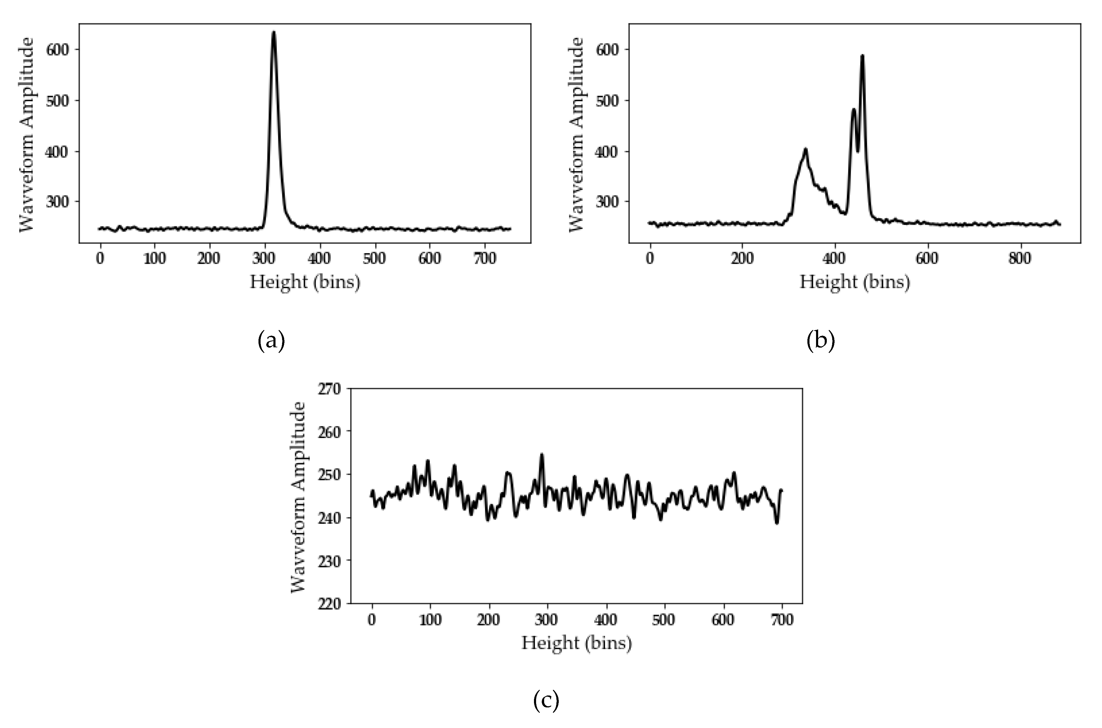
This section will begin with an analysis of two exemplary GEDI waveforms acquired on lakes (
Figure 2). Then, the remainder of the results section will analyze the quality of the GEDI elevations for each lake, date, and finally for each beam.
Figure 2a shows a perfect example of a viable GEDI waveform over water surfaces (usable waveform with a high signal-to-noise ratio). The waveform presents a single distinct peak corresponding to the water surface, with very low noise level. In contrast,
Figure 2c shows a GEDI waveform with very high noise level and no distinctive peaks, which renders such waveforms useless. The example waveform shown in
Figure 2c could correspond to acquisitions in the presence of clouds over our study area.
The comparison between GEDI elevations and in-situ elevations registered from the hydrological gauge stations shows that the parameters used in algorithm a1 (Smoothwidth_zcross of 6.5 ns,
Table 2) provide more precise elevations in comparison to algorithm a2 (Smoothwidth_zcross of 3.5 ns,
Table 2). Using the entire database from all the lakes in this study (8 lakes and 4637 viable waveforms), GEDI footprint elevations in comparison to in-situ gauge station elevations showed a mean elevation difference of 0.61 cm with a1 and 7.8 cm with a2. The standard deviation of the mean difference between GEDI footprint elevations and gauge station readings is 22.3 cm using a1 and 23.7 cm using a2. The root mean square error (RMSE) on GEDI elevations is slightly higher using a2 with a value of 24.9 cm against 22.3 cm using a1.
3.1. Analysis of GEDI Waveforms for Each Lake
The precision of elevations estimated from GEDI waveforms was studied separately for each lake using all GEDI beams from all acquisition dates.
Table 3 shows a mean difference (MD) between GEDI and in-situ elevations that varies between −13.8 cm (under-estimation by GEDI) and +9.8 cm (over-estimation by GEDI). The reported standard deviation from MD varied between 14.5 cm and 31.6 cm.
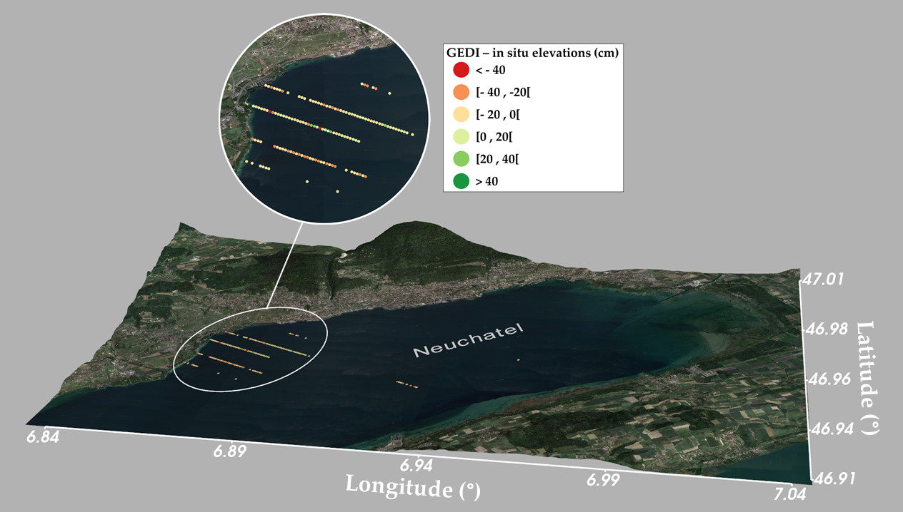
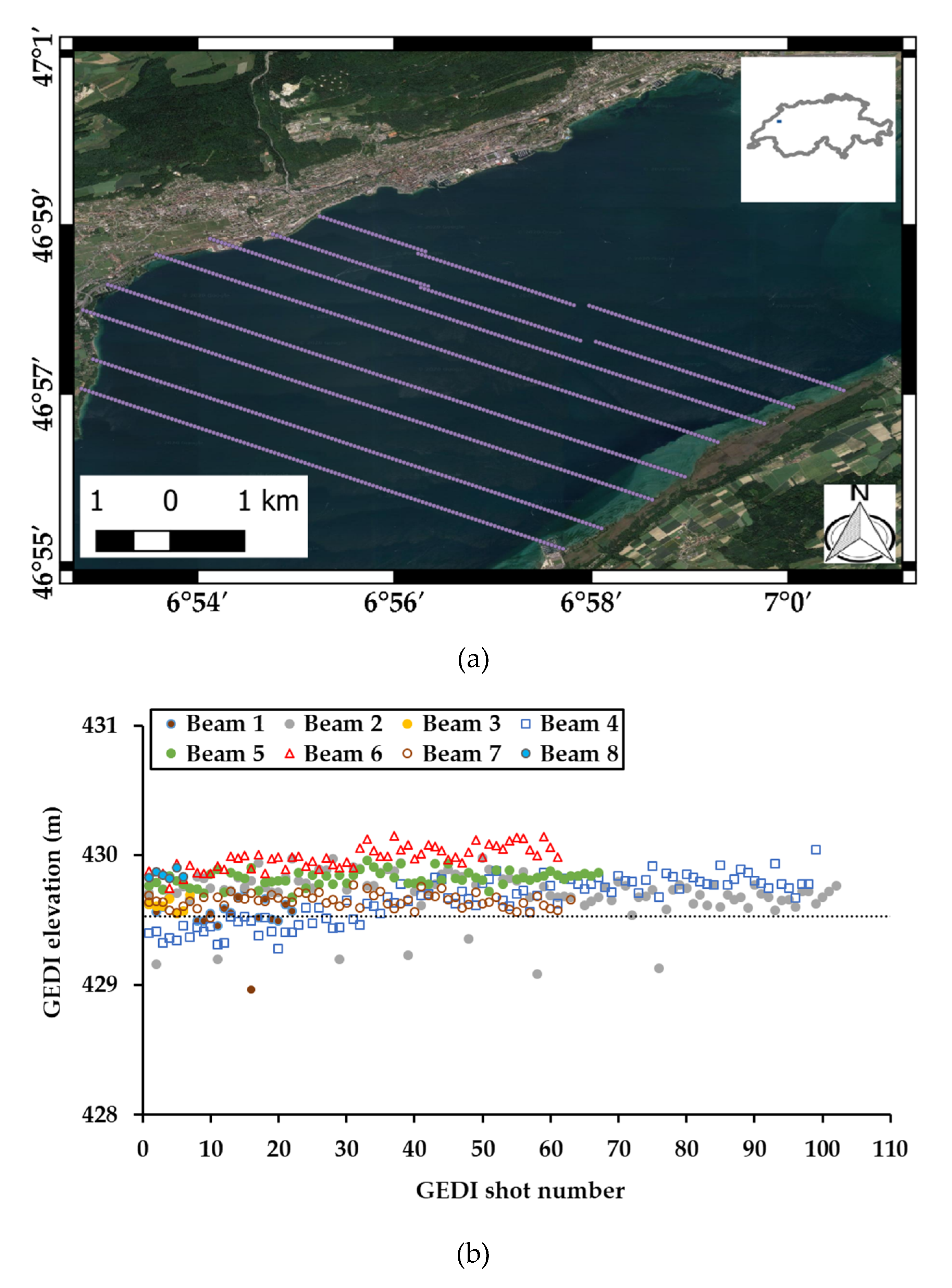
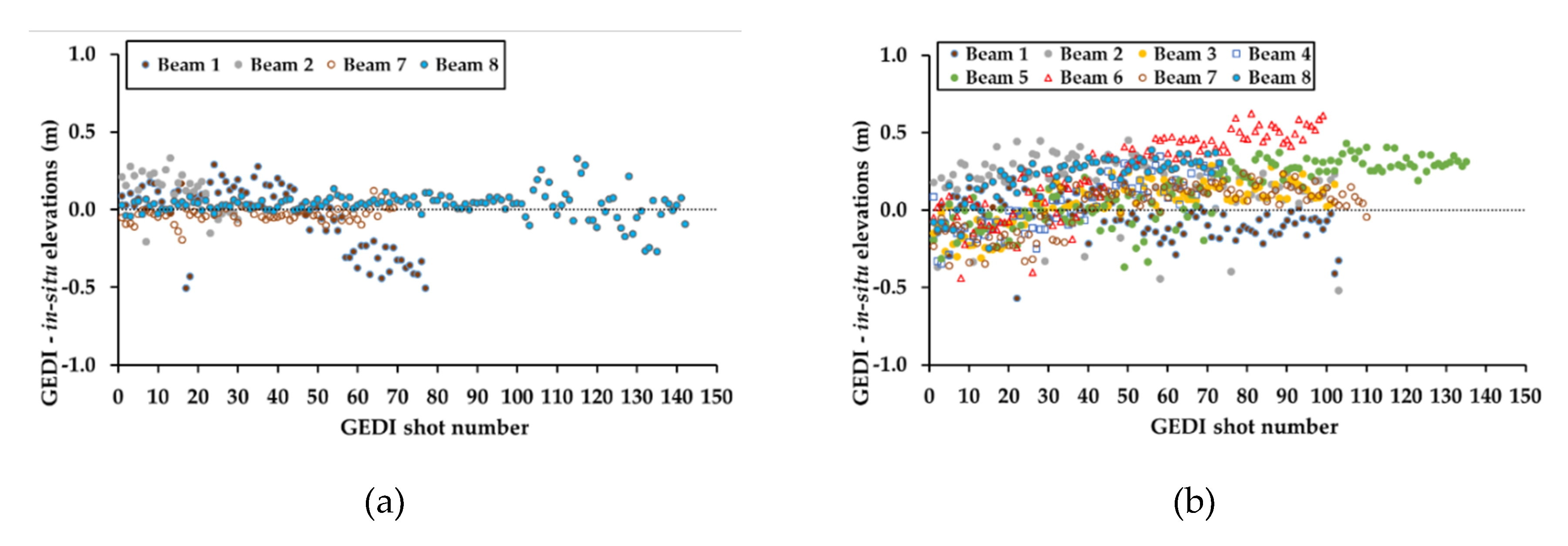
Figure 4a shows an example of GEDI data for a transect with its 8 beams, acquired on May 29th 2019 at 9:25 p.m. over lake Neuchâtel in Switzerland (GEDI elevations for all lakes can be found in
Appendix A,
Figure A1). This example shows what has also been observed over the other lakes, albeit with different elevation precision depending on the acquisition date, or beam. Over the transect in
Figure 4a, the mean difference (MD) between elevations from GEDI and those reported by the gauge station varied between −6.4 (under-estimation by GEDI) for beam 1 and +45.2 cm (over-estimation by GEDI) for beam 6 (
Figure 4b). The standard deviation from MD varied between 5.5 cm for beam 7 and 17.5 cm for beam 4. Using elevations from all the beams acquired on May 29th 2019 over Lake Neuchâtel, the calculated MD was in the order of +6.1 cm (over-estimation by GEDI) with a standard deviation of 16.1 cm. Moreover, over some GEDI footprints, we observed on some beams, elevations that deviated greatly from the mean of all GEDI elevations, with some of these elevations being 50 cm further from the mean. Despite all verification, we were unsuccessful in explaining the reason for such elevation differences, even though these points were acquired in the middle of the lake, and their corresponding waveforms showed very high signal to noise ratio, and resembled in form to other waveform from other footprints.
3.2. Analysis of GEDI Waveforms by Date
Table 4 shows the mean difference and the standard deviation between elevations from GEDI and in-situ gauge records, using data over all lakes, grouped by date. Results show that the mean difference (MD) between elevations from GEDI and in-situ gauges varied between −26.8 cm (under-estimation by GEDI) and +15.2 cm (over-estimation by GEDI). The lowest bias corresponded to data acquired the mornings of April 28, and May 02 and 04, or late at night on May 22. The highest recorded bias was observed on acquisitions that were made around noon (e.g., April 21, May 28, and June 08), in the early evening (May 29), GEDI acquisitions taken over the weekend (e.g., April 20 and 21, June 08), or before a holiday (e.g., May 22). These strong biases could be due to several phenomenon. (1) Increased perturbations of the water surface due to human activities taking place at these times. The reported standard deviation from MD shows that it varies between 12.7 cm and 24.9, with a standard deviation lower than 15 cm for morning acquisitions (e.g., April 28, May 02, and 04), with the exception of June 08, which corresponds to acquisitions taken around noon. (2) Currents generated by thermal effects or winds [
35,
36].
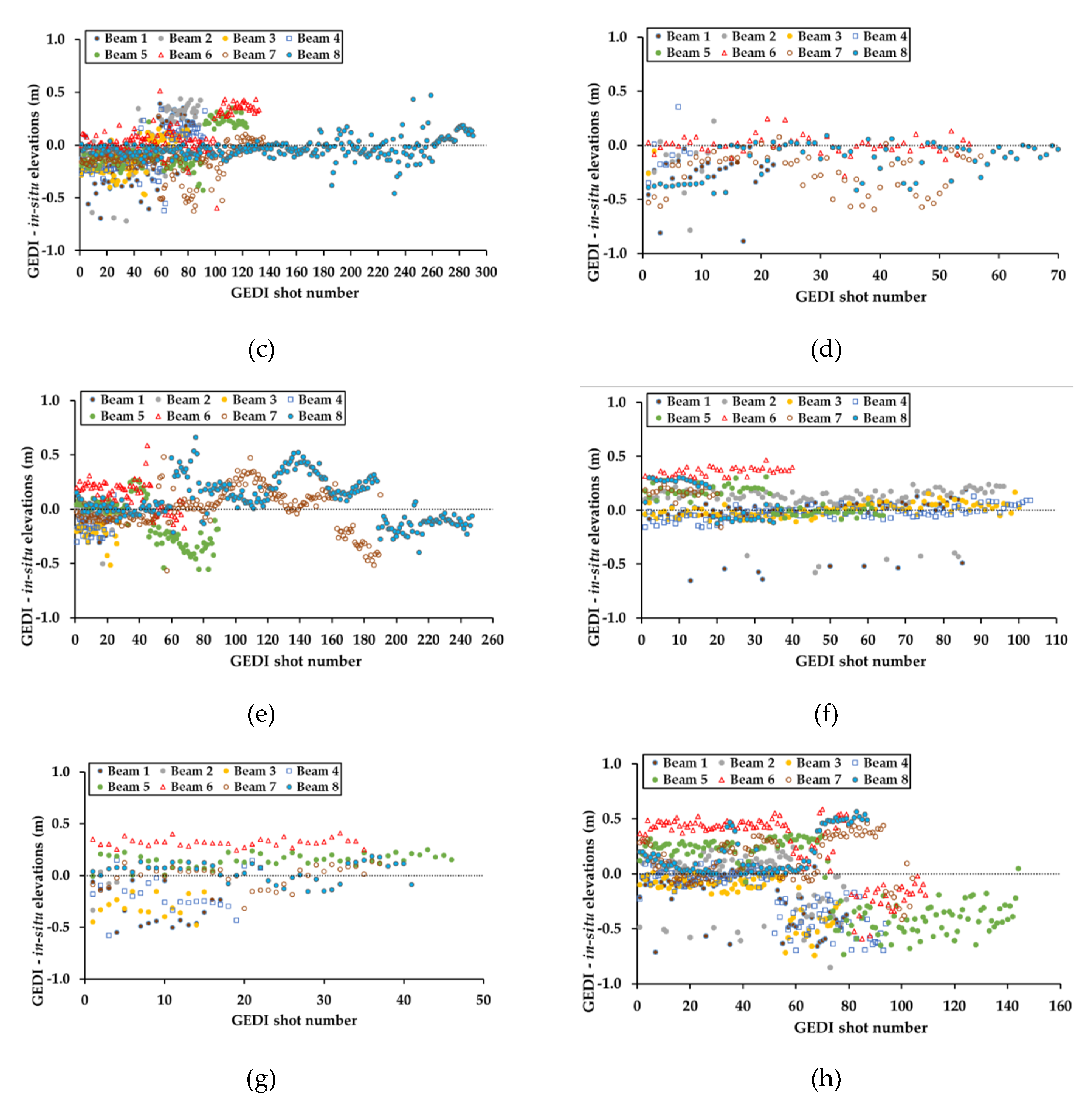
3.3. Analysis of GEDI Waveforms by GEDI Beam
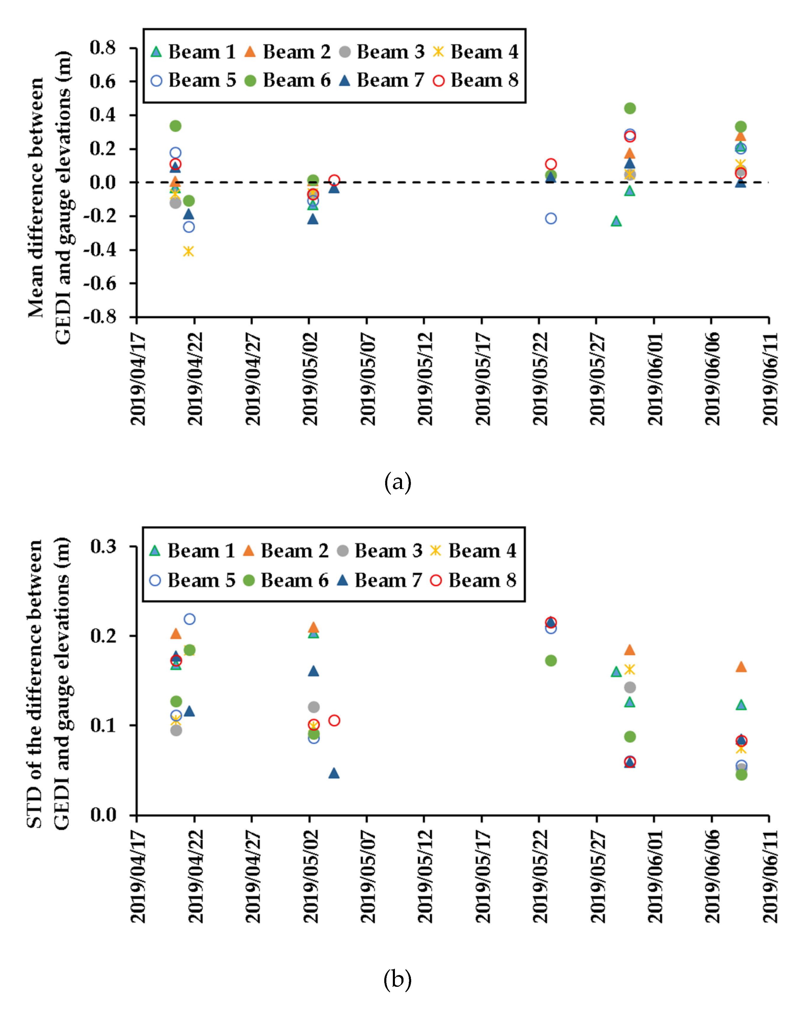
Figure 5 shows the summary of the statistics calculated from the difference between GEDI and hydrological gauge elevations for each date and each beam, using data from all lakes. These statistics were first calculated for each GEDI beam and for each date. Only the statistics with at least 30 GEDI shots for each date/beam pair are reported in this section. Results show that the bias (elevations from GEDI—elevations from gauge stations) varied depending on the acquisition date, and the beam. For certain beams, at certain dates, elevation from GEDI had the same order of magnitude as in-situ elevations, while, for other dates, and even for the same beam, the bias was very significant (
Figure 5a). For example, on 20 April 2019, elevations from GEDI acquired over beam 1 showed a bias of −2.9 cm which increased to +21.9 cm on 8 June 2019. Similarly,
Figure 5b shows that the standard deviation from the mean difference between GEDI and gauge station elevations varied between 4.6 cm (beam 6, 8 June 2019) and 22 cm (beam 5, 21 April 2019).
The statistics were then calculated for each GEDI beam, using all the dates. Results in
Table 5 show that the difference between elevations from GEDI and in-situ gauge records differed according to the laser they were acquired with. The mean difference between GEDI and in-situ elevations varied between −10.2 cm (under-estimation by GEDI) and +18.1 cm (over-estimation by GEDI). The beams with the highest difference were beams 1 (coverage beam) and beams 6 (full power beam) with a mean difference of, respectively, −10.2 cm and +18.1 cm. In contrast, the beams that captured elevations with the smallest diversion from in-situ elevations were beams 5 and 7 (both full power beams), with a mean difference of −1.7 cm, and −2.5 cm, respectively, while the remaining beams (2, 3, 4, and 8) show the mean observed difference varied between −7.4 cm and +4.4 cm. Finally, the standard deviation from the mean difference between elevations from GEDI and elevations from in-situ gauges were similar across beams, with a standard deviation that varied between 17.2 cm and 22.9 cm.
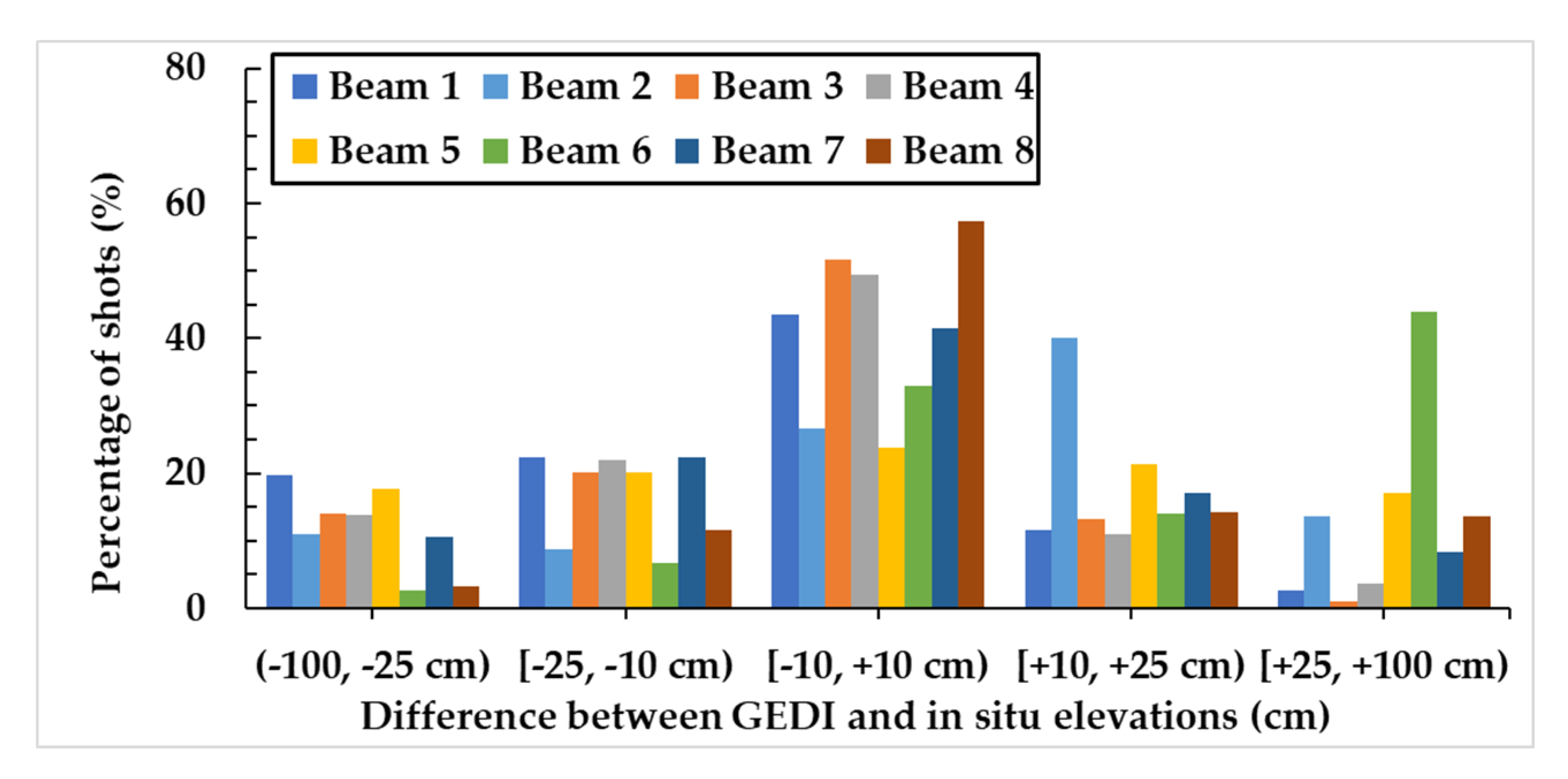
Finally, we present an analysis of the distribution of the difference between GEDI elevation estimates for each beam in comparison to in-situ elevations. The difference (D) between GEDI and in-situ elevations has been grouped into five intervals: (−100, −25), [−25, −10), [−10, +10), [+10, +25), and [+25, +100) cm.
Figure 6 shows that the lowest elevation differences were obtained using beams 3, 4, and 8. Overall, GEDI elevations from beam 8 were the most accurate, followed by beams 3 and 4, then beams 1, 2, and 7, and finally beams 5 and 6 showed large differences between elevations from GEDI and those from in-situ gauge stations. For beam 8, 57% of the shots had a difference with in-situ elevations between −10 and 10 cm, followed by a small percentage of shots with D between −100 and −10 cm and between 10 and 100 cm. For beams 3 and 4, the difference between GEDI and in-situ elevations was between −10 and +10 cm for ~50% of the shots, with a small percentage of shots with D between +25 and +100 cm (less than 5%), and between −100 and −25 cm (~14%). The difference in elevations D for beams 1, 2, and 7 was between −25 and +25 cm for, respectively, 78, 75 and 81% of the shots. Finally, for beam 6, 44% of the shots showed very high over-estimation of GEDI elevations (D between +25 and +100 cm), while, for beam 5, the elevation differences were distributed almost equally among the five classes of D. Moreover, results showed that almost 43% of the shots with an elevation difference D in the range (−100, −25 cm] or in the range [+25, +100 cm) were obtained from beams 5 and 6 (19.7% from beam 5, and 22.1% from beam 6). In contrast, only 5.3% and 6.5% of shots in beams 3 and 4 showed an elevation difference D in the range (−100; −25 cm] or in the range [+25;+100 cm).
3.4. GEDI Waveform Metrics and Elevation Accuracy
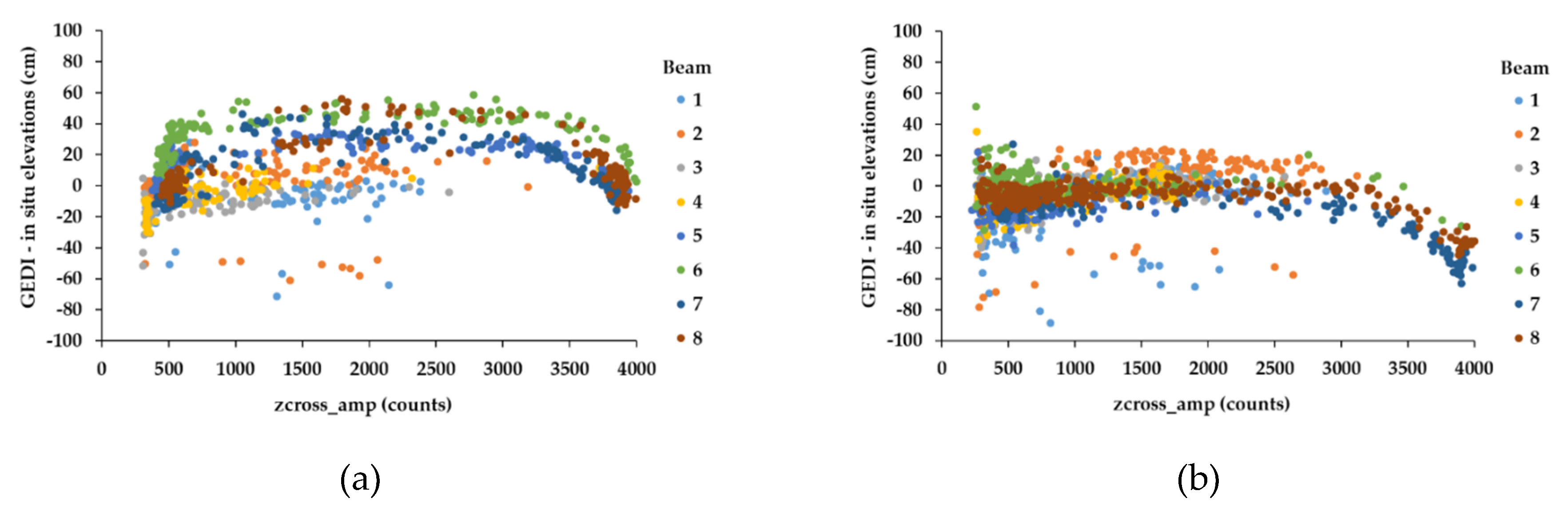
In this section, we present the effect of some GEDI waveform metrics that could potentially be affected by sensor saturation, and thus have an effect on the GEDI elevation estimations. The correlation between the amplitude of the smoothed waveform at the lowest detected mode (zcross_amp from the L2A product) and the precision on the elevation has been analyzed. This analysis was carried on only two dates (20 April, and 02 May) which had the maximum number of GEDI acquisitions (~1000 shots for each acquisition date). On April 20th (
Figure 7a), the variable zcross_amp varied between 280 and 4000 amplitude counts (AC). For zcross_amp between 280 and 600 AC, the difference D (difference between GEDI and in-situ elevations) increased with zcorss_amp from −50 to about +40 cm. For zcross_amp between 600 and 3000 AC, the difference D was stable with a value around +50 cm for beam 5 and 0 cm for beam 3. For values of zcross_amp between 3000 and 4000 AC the difference between GEDI and in-situ elevations decreased from +40 cm to around −10 cm. A similar pattern was observed for acquisitions taken on 2 May 2019 (
Figure 7b), especially for zcross_amp between 3000 and 4000 AC. For zcross_amp between 600 and 3000 AC on May 2, the difference D was stable and was around 0 cm. However, it decreased to −60 cm for zcross_amp around ~4000 AC. For zcross_amp, less than 600 AC, the difference D remained stable but with strong fluctuations for low zcross_amp values (zcross_amp less than 400 AC). The increased uncertainties for waveforms with higher values of zcross_amp (higher than 3000 AC) are most probably due to the specular reflection of the water that saturates the detector [
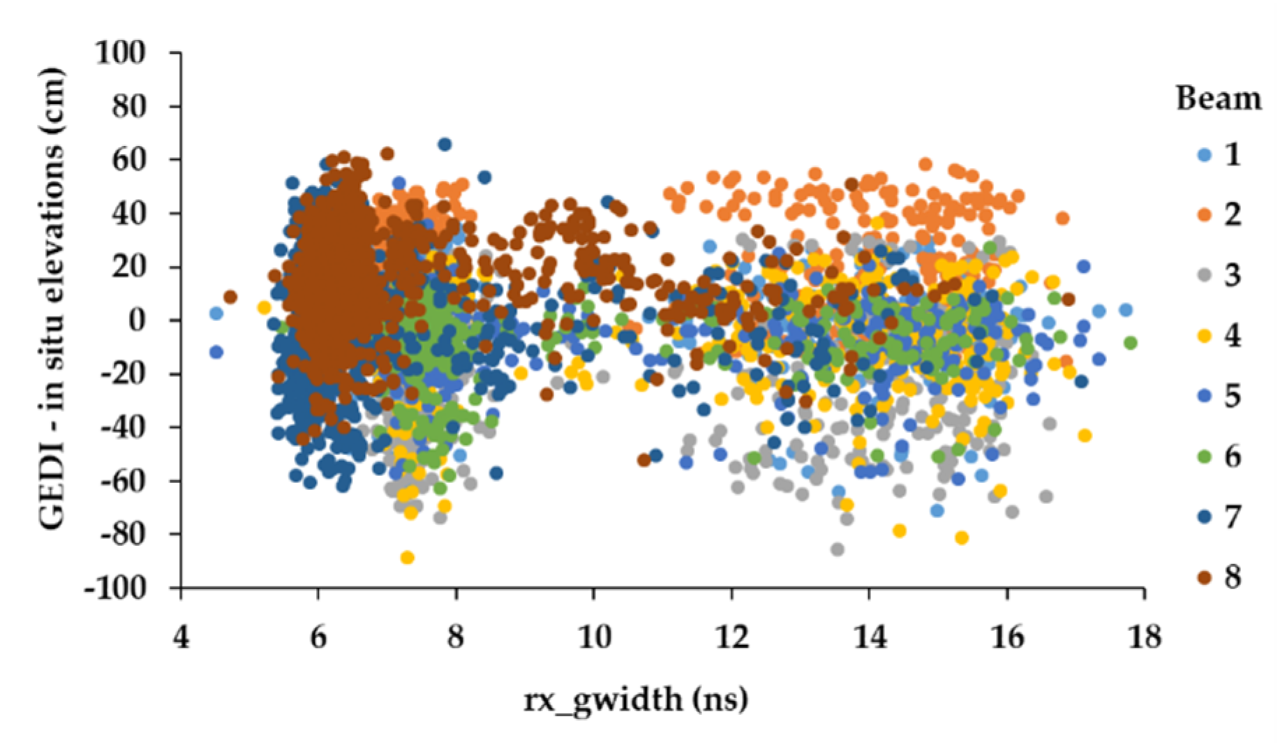
29]. Moreover, a large portion of the waveforms with zcross_amp higher than 3000 AC were also observed as having a wider peak which indicates some form of saturation. Indeed, the analysis of the difference D and the width of Gaussian (width of the return peak in the case of unimodal waveforms) fit to the received waveforms (rx_gwidth, available in the L2A data product) shows two clusters (
Figure 8). The first cluster corresponds to rx_gwidth values between 4.5 and 9 ns, and the second cluster corresponds to rx_gwidth between 11 and 17 ns.
Figure 8 shows that the waveforms from the second cluster have a slight under-estimation of elevations of around 10 cm.
3.5. Modelling GEDI Estimation Erorrs
In the previous sections, we showed that there were several instrumental and environmental factors affecting the acquired GEDI waveforms, thus producing an important difference between in-situ and GEDI estimated elevations. Among these factors, the provided zcross_amp, rx_gwidth from the L2a data product, and the derived GEDI viewing angle (
) has been examined. zcross_amp and rx_gwidth were chosen as they are an indicator of saturation as seen in the previous section, whereas the viewing angle has been demonstrated in Urban et al. [
37] to increase elevation errors for ICESat-1 GLAS when the viewing angle deviates from nadir due to precision attitude determination. In this paper, the GEDI viewing angle (
) has been estimated using the following equation:
where
d is the distance between an acquired GEDI shot and the position of GEDI projected at nadir onto the WGS84 reference ellipsoid and
H is the elevation of GEDI over the referenced ellipsoid.
In addition to the previous factors, several additional environmental factors have also been considered since in-situ water levels do not necessarily provide water elevation across the surface of lakes as standing waves (seiches), and wind-generated waves are commonly present over lakes. Over the studied lakes, no direct information about waves were available, therefore, they were substituted by proxy variables. In essence, we chose the factors that influence the creation and the form of standing, and wind-generated waves (e.g., wave heights and wave direction). These factors include wind speed, wave direction, and lake depth. Wind speeds were acquired at each GEDI acquisition date using meteorological data from the nearest weather stations. Wave direction and average lake depth at each GEDI footprint were acquired from the LATLAS project (swisslakes.net) using GEDI footprint coordinates for lake depth, and wind direction and GEDI footprint coordinates to determine the wave direction. Nonetheless, these factors were only available for five of the eight studied lakes (Geneva, Neuchâtel, Zürich, Obersee (Zürich), and Lucerne).
In
Section 3.2, it was shown that GEDI acquisition dates and times could influence the accuracy of GEDI elevation estimates. Therefore, two additional factors were considered for the modelling of GEDI estimation errors. (1) The acquisition time of a GEDI shot (Time of Day, TOD) was converted to a value between 1 and 3 representing, respectively, acquisitions taken in the morning (6 a.m. to 12 a.m.), afternoon (12 a.m. to 6 p.m.), and evening (6 p.m. to 12 p.m.). (2) The acquisition date of a GEDI shot was converted to a value between 1 and 7 representing the acquisition day (Day of Week, DOW).
Finally, GEDI estimation errors were modeled using the previously mentioned factors in a Random Forest regressor (RF). Random Forests are an ensemble of machine learning algorithms used for classification or regressing by fitting a number of decision trees on various sub-samples of the dataset, and uses averaging to improve the predictive accuracy and control over-fitting [
38]. Compared to linear models, RF is advantageous for being able to model also nonlinear relationships (threshold effect) between the variable to explain and the explanatory variables. For this study, the number of trees in the RF were set to 100 trees, with a tree depth equal set to the square root of the number of available factors. In order to train and assess the model accuracy, we randomly split the database into 70% for training and 30% for validation (and accuracy estimation).
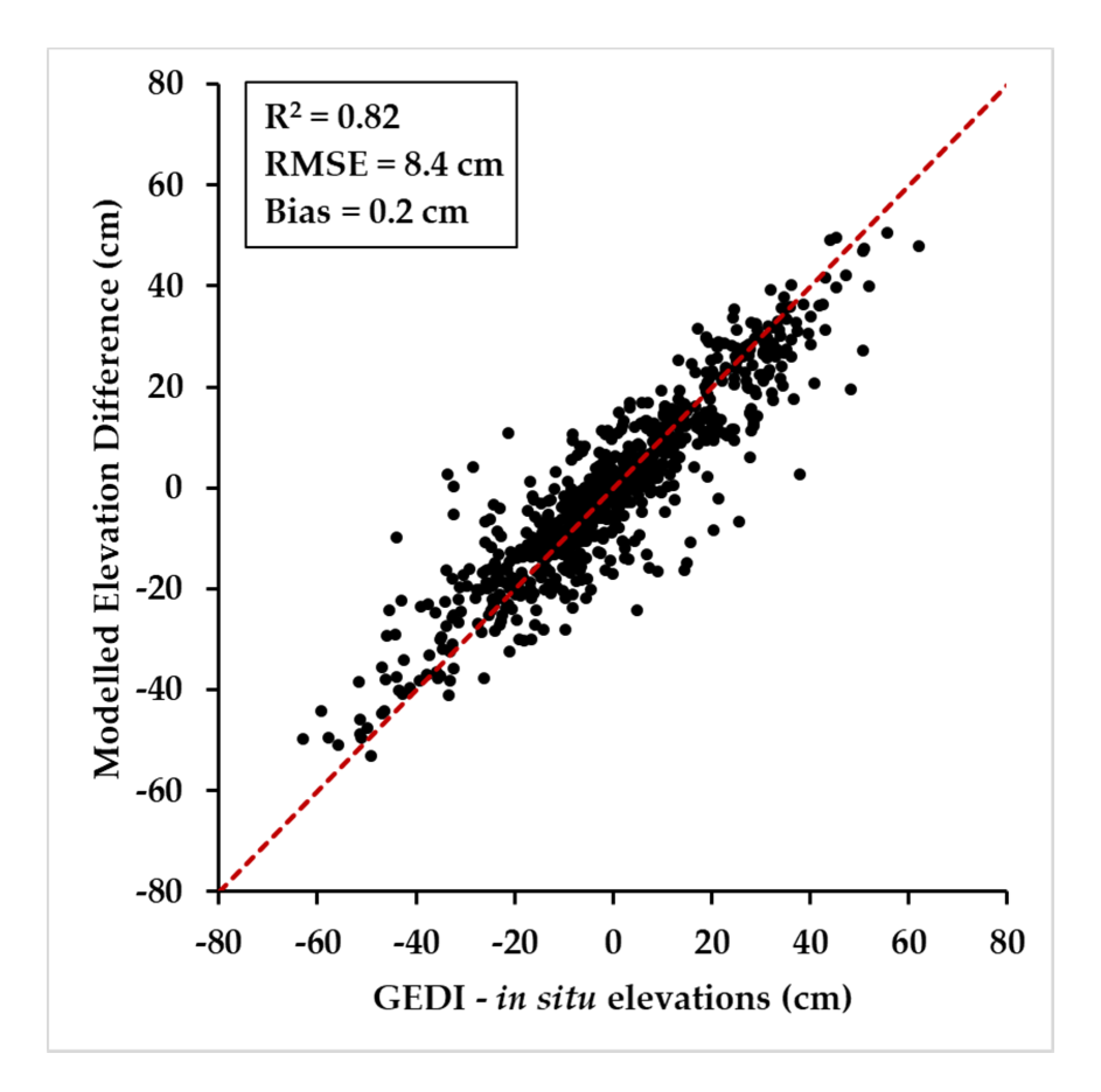
The random Forest regression results for the five lakes combined showed that we were able to explain ~82% of the error (GEDI—in-situ elevations) variance and reduce the RMSE on the elevation estimation from 20.2 to 8.4 cm (
Figure 9).
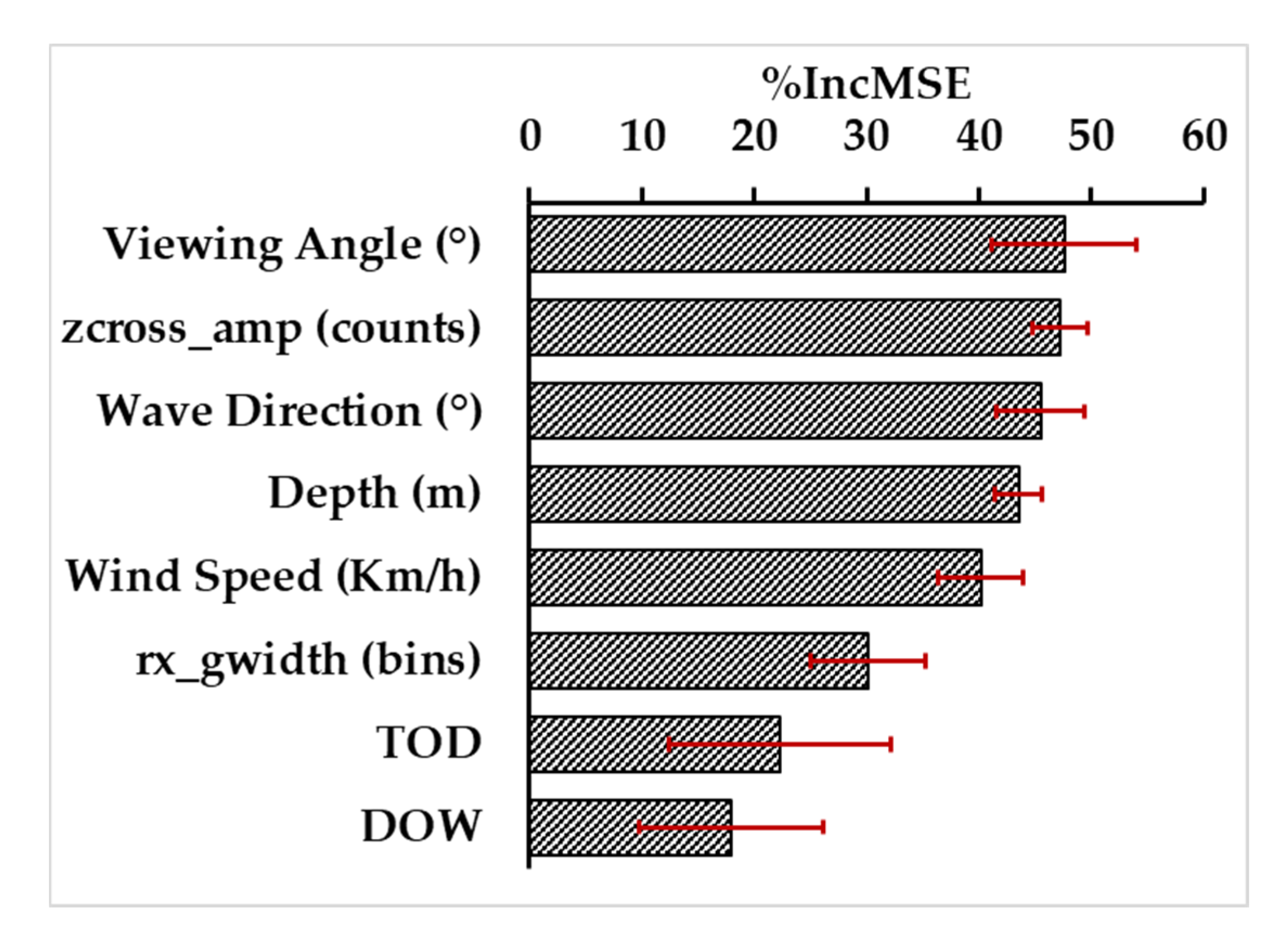
Moreover, the factors that contributed the most on the difference between GEDI and in-situ elevations were determined. This process was conducted using the percentage increase in the mean square error of the regressions (%IncMSE, estimated with out-of-bag cross validation) from the factor importance test for the random forests model (average and standard deviations of 50 repetitions) (
Figure 10). The factor importance test shows that the most important factors for the modeling of errors is related to the viewing angle of GEDI (47.6%), followed by zcross_amp (47.2%) wave direction (45.5%), depth (43.5%), wind speed (40.2%), and rx_gwidth (30.2%). The least important factors are the effect of the acquisition time (TOD 22.3%) and date (DOW 18.0%).
The modeling of GEDI errors for each lake separately did not show any differences specific to the location, geography, or geometry of the lake. For the five lakes tested, the random forest regressor was able to explain between 70.1 to 83.3% of the error (GEDI—in-situ elevations) variance, with an accuracy on the GEDI elevations between 5.6 and 10 cm (
Table 6).
4. Discussion
Using GEDI data extracted from the algorithms developed by the GEDI team, the accuracy of the GEDI water surface elevation estimates seems to be high enough. Overall, the standard deviation from the mean difference between GEDI and in-situ elevations is ~22 cm with no apparent bias. Moreover, given GEDI’s small footprint diameter (25 m), GEDI should provide better elevation estimates in comparison to, for example, radar altimeters for narrower water surfaces, such as rivers. On the other hand, while GEDI uses the same laser specs as those used for GLAS on board ICESat-1, the precision obtained by GEDI is inferior to that obtained using ICESat-1. In fact, Baghdadi et al. [
29] in their study over Swiss lakes, observed an accuracy (RMSE) of elevation estimates in the order of ~5 cm using ICESat-1 data.
GEDI’s smaller footprint means that GEDI waveforms within the footprints could easily be affected by small disturbances coming, for instance, from water surface roughness, which leads to uncertainties in the estimation of water surface elevations. For example, GEDI acquisitions with the highest mean difference to in-situ elevations, and highest standard deviation were acquisitions taken during the weekend (e.g., April 21, June 08), or before a holiday (e.g., May 22). The uncertainties at these acquisition dates could be explained in part by the increased human activities over the water surface (e.g., ships) which pollutes the return waveform. Moreover, these uncertainties are also the result of small currents generated by thermal effects [
35] or winds [
36], that disrupts the water surface. Finally, over large lakes, water surface is not entirely flat due to the presence of wind-generated waves and seiches. Therefore, GEDI, depending on the angle of incidence, can over- or under- estimate the water surface level by providing elevations from the trough or the top of the waves. In our study of the effects of GEDI’s viewing angle over each lake and each date, we observed that, generally, uncertainties on the estimation of elevations increased with increasing viewing angle. Moreover, the acquisitions with the large deviation to the mean elevation difference between GEDI and in-situ elevations were acquisitions with the largest viewing angle.
The time of GEDI acquisitions also introduces uncertainties on the elevation estimates. For example, during sunlit GEDI acquisitions, photons from the sun reflecting at the water surface could contaminate the returned echo and increase the noise. In this study, we found that GEDI elevation estimates with the lowest standard deviation and bias to the in-situ elevations were acquisitions taken during the morning or late at night when lake water surfaces are usually calm, cooler with low wind speeds. For these acquisition times (April 28 and May 02, 04, and 22), the mean difference between GEDI and in-situ elevations was −6 ± 15 cm.
The analysis of the precision of elevations from GEDI according to the used laser in the acquisition did not show any difference between coverage and full power laser. Nonetheless, some beams showed systematic differences in comparison to others. In general, the most accurate elevations came from beams 1–4 (coverage laser) and beams 7–8 (full power laser). Beams 5–6, which also correspond to a full power laser, showed the least precise elevations across all dates. Moreover, there were some differences on the elevation estimation accuracies across the beams. For example, footprints acquired from beam 8 had better precision than footprints from beam 7, albeit both beams are produced using the same laser unit onboard GEDI. Similar observations have been noted for beams 3 and 4, which were found to be more precise than beams 1 and 2. However, these uncertainties could be mostly explained by the errors introduced from the viewing angle of GEDI, which differs from one beam to another on a given acquisition date.
In general, the differences between GEDI and in-situ elevations are due to both instrumental and environmental factors. In our modeling of the errors, the two most contributing factors were the viewing angles of GEDI, and the saturation on some of the acquired waveforms assuming this occurs through the zcross_amp indicator. However, these factors could be corrected in unimodal waveforms. Another form of uncertainties is related to the uneven water surface due to standing and wind-generated waves. This was apparent by the high contribution of environmental factors, like the wave direction, depth of the lake at each GEDI footprint, and the wind speed. Lake depth is a direct indicator of the wave heights as waves near the shore (low depth) are higher than waves farther away, while wind speed controls the height of the generated wave. In this study, the contribution of wind speed on the errors appears to be lower than other factors. However, this is due to the low wind speeds at the present GEDI acquisition (maximum encountered wind speed of 12 km/h), which suggests small wind-generated waves. In addition to instrumental and environmental factors, the acquisition date and time of GEDI can also directly affect its accuracy. The time of the acquisition during the day, as well as the day of the week on which an acquisition took place, both can have effects on the echoed waveforms as seen previously. The effect of these two factors is related to the noise from the sun on the GEDI receiver, and the increased human activities over each lake during certain days.
Finally, the provided quality_flag from the L1B data product could help, in theory, to select GEDI data with higher accuracy on elevations. Using data issued after the application of our filter (|SRTM elevation—GEDI elevation| > 100 m), we observed only a slight decrease of the root mean square error on GEDI elevation estimates when we considered only the waveforms with a quality_flag = 1. For algorithm a1, we observed a decrease in the RMSE of around 1.4 cm (from 22.3 cm using data with both quality_flag = 0 and 1 to 20.9 cm using only quality_flag =1). Similarly, for a2, the decrease in the RMSE was around 0.8 cm (from 24.9 cm using data with both quality_flag = 0 and 1 to 24.1 cm using only quality_flag = 1).
5. Conclusions
In this study, we analyzed GEDI data in order to determine its accuracy of elevation estimation over lake surfaces using algorithms provided by the Land Processes Distributed Active Archive Center (LP DAAC). The objective was to study the quality of the first two months of GEDI data (min-April until mid-June 2019) acquired over several lakes in Switzerland. Overall, 4367 GEDI shots out of 21,242 available shots were exploitable and analyzed over the eight studied lakes.
This first analysis of GEDI data from the first two months of acquisitions showed a very low mean elevation difference between GEDI and in-situ gauge station elevations, in the order of 0.61 ± 22.3 cm for one standard deviation. While GEDI’s reported vertical accuracy in this study was well below the 50 cm vertical accuracy provided in Dubayah et al. [
31], it still remains higher than what was previously obtained using the ancient LiDAR satellite ICESat-1. In fact, the vertical accuracy of GLAS onboard ICESat-1 was better than 10 cm, as demonstrated by Baghdadi et al. [
29].
The analysis of GEDI data by lake showed that the vertical precision varied from under-estimation by GEDI of −13.8 cm for certain lakes, to over-estimations of +9.8 cm for others, with a varying standard deviation between 14.5 and 31.6 cm.
The investigation of GEDI’s vertical accuracy by date showed a mean difference between GEDI and in-situ gauge station elevations varying between −26.8 and +15.2 cm. The lowest bias corresponded to data acquired in the morning or late at night. The highest recorded bias was observed on acquisitions that were made around noon, in the early evening, and over the weekend. Moreover, the difference in GEDI’s elevation accuracy according to the acquisition date is also affected, in part, by the instrument’s viewing angle at acquisition time (larger viewing angle leads to lower accuracies). However, the full effects of the viewing angle were not studied in its entirety due to the small number of available acquisitions at the time of this writing.
The analysis of GEDI data by beam number showed that the difference between GEDI and gauge stations’ elevations varied depending on the acquisition date and the beam. Certain beams at certain dates showed that elevations from GEDI were very similar to in-situ readings (fluctuations of few cm). Summary statistics calculated for each GEDI beam using acquisitions from all dates showed that the beams with the highest elevation differences to in-situ readings were beams 1 and 6 (−10.2 and +18.1 cm, respectively). In contrast, the beams with the smallest mean elevation difference to in-situ readings were beams 5 and 7 (−1.7 and −2.5 cm, respectively). The remaining beams (2, 3, 4, and 8) showed a mean difference between −7.4 and +4.4 cm. The standard deviation of the mean difference, however, was similar across all beams (between 17.2 and 22.9 cm).
The analysis of the metrics, such as the amplitude or width of the modes, did not allow further investigation of GEDI elevation estimation accuracy, even though a certain dependence was found between these metrics and the quality of GEDI data.
Nonetheless, accounting for instrumental and environmental factors increased the accuracy (RMSE) of GEDI estimates to 8.4 cm for all lakes and from 5.6 to 10 cm (with no apparent bias) when modeling the errors for each lake independently.
Following the first analysis done on the first GEDI data sets, we can conclude that GEDI has a strong potential for precise estimation of water surfaces of any size. Moreover, a better estimate of GEDI metrics by the LP DAAC can be expected in the near future, allowing for reprocessed data with a better elevation precision.


 ,
, 


