Automatic gbXML Modeling from LiDAR Data for Energy Studies


Abstract

1. Introduction
2. Materials and Methods
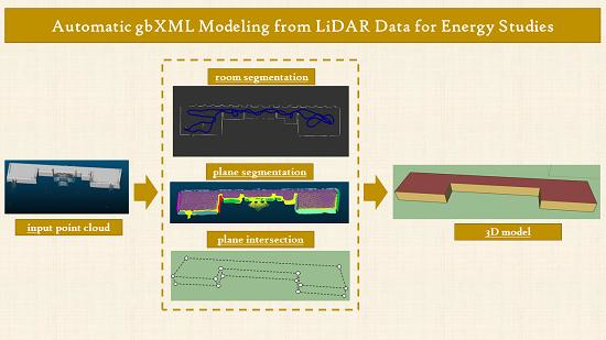
2.1. Geometric Modeling
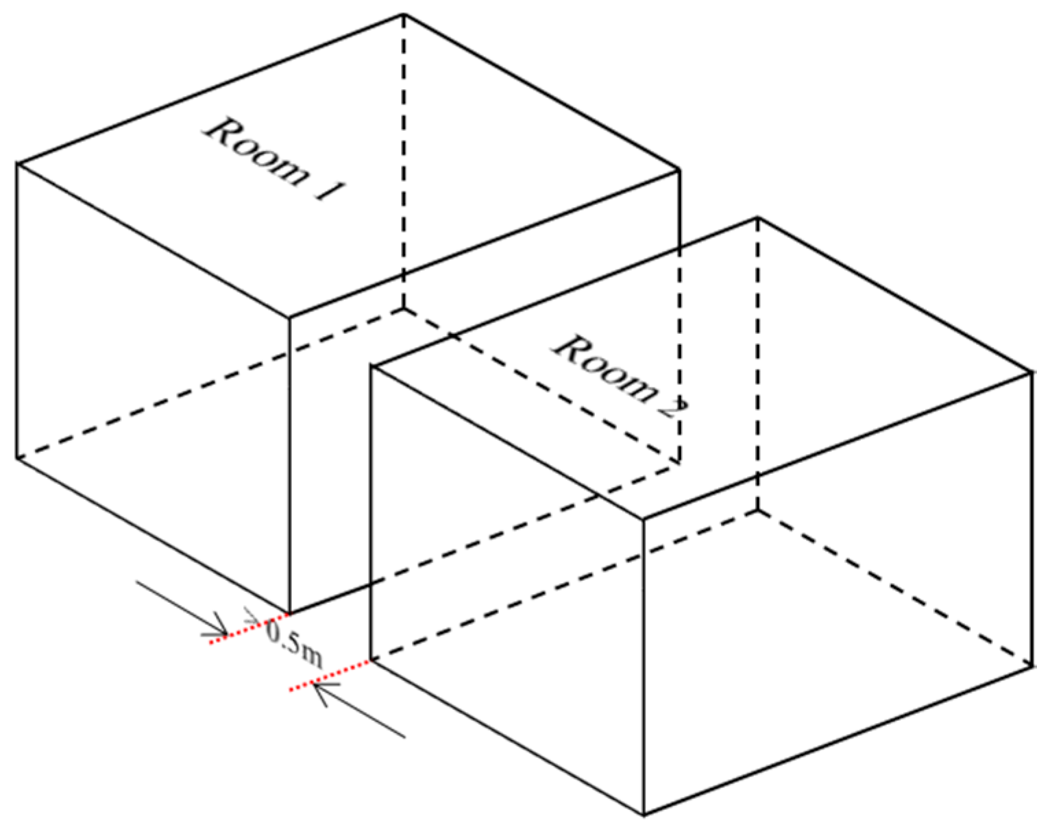
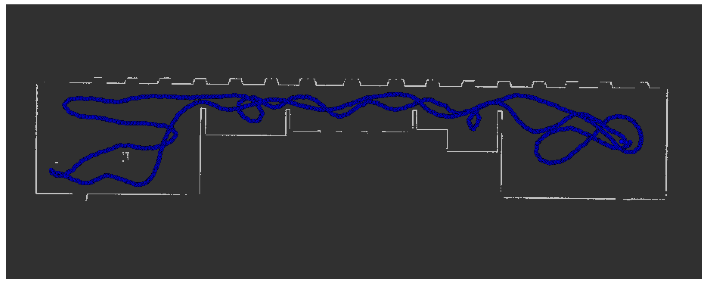
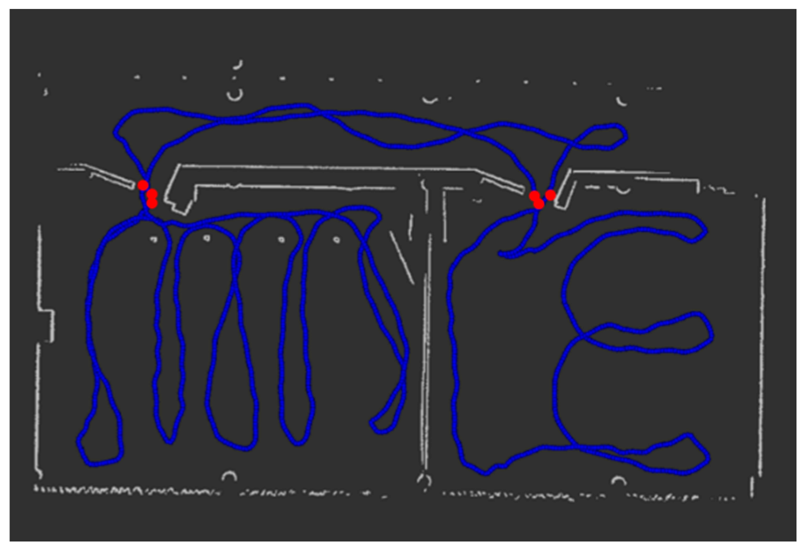
2.1.1. Room Segmentation
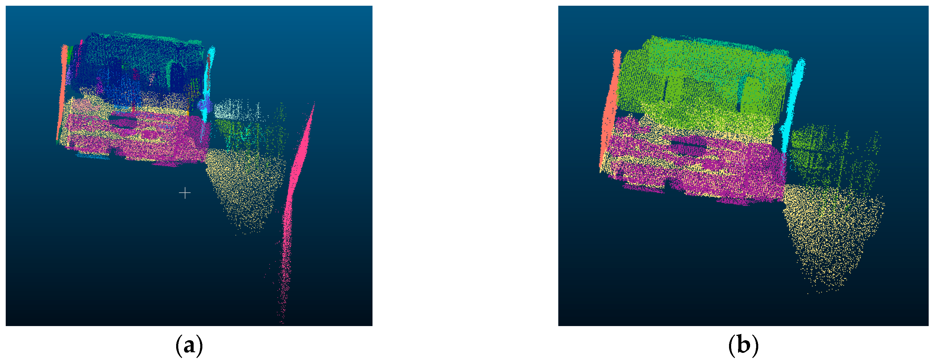
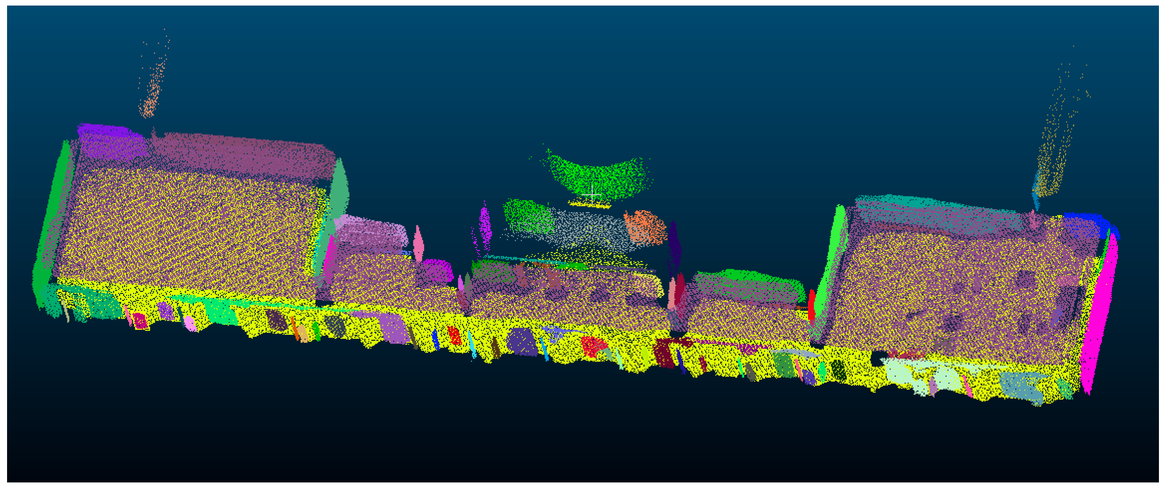
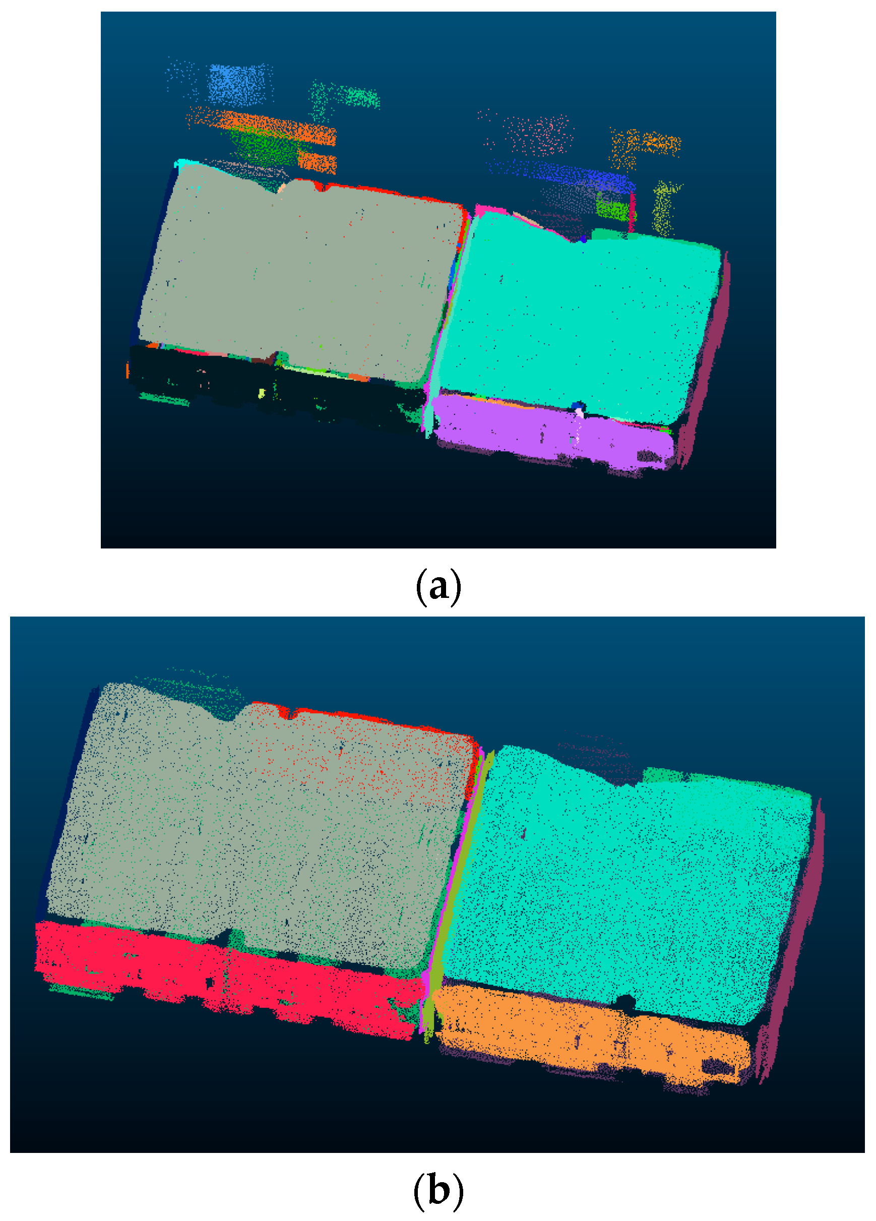
2.1.2. Plane Segmentation
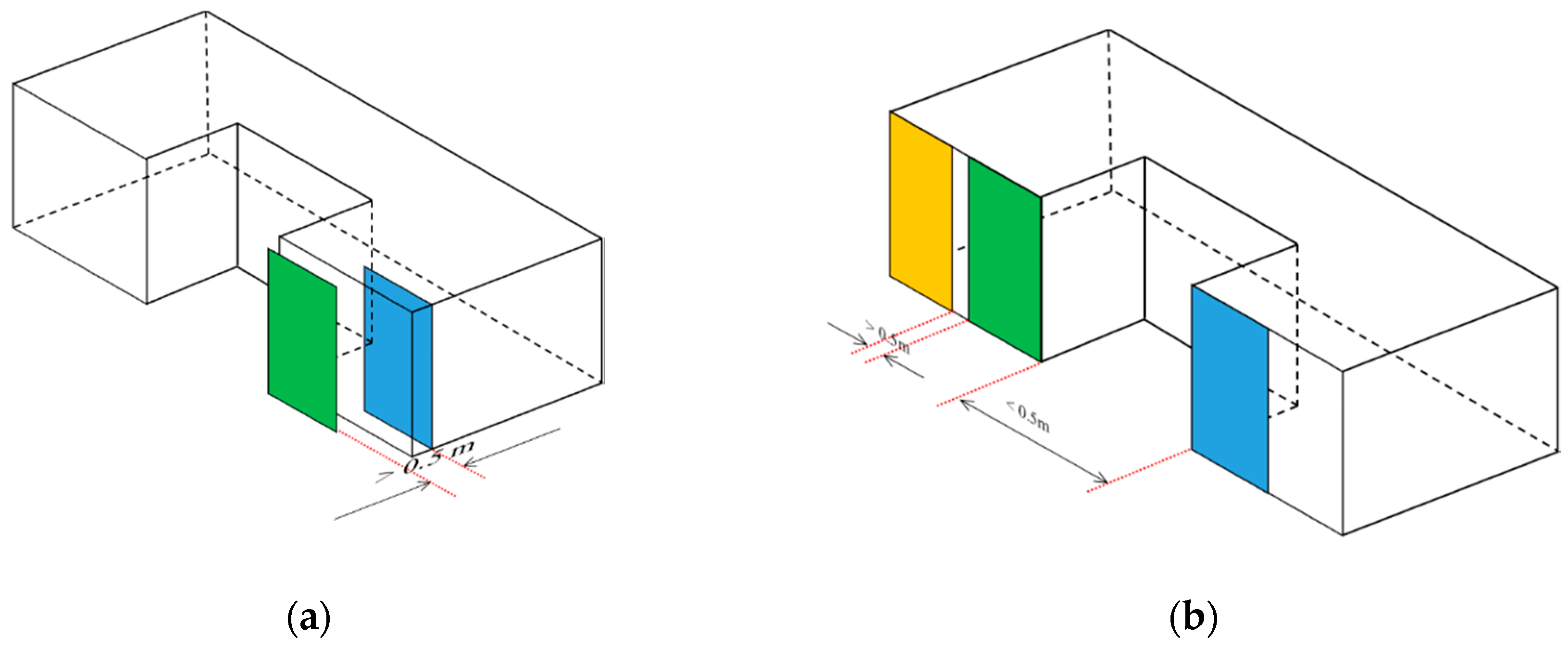
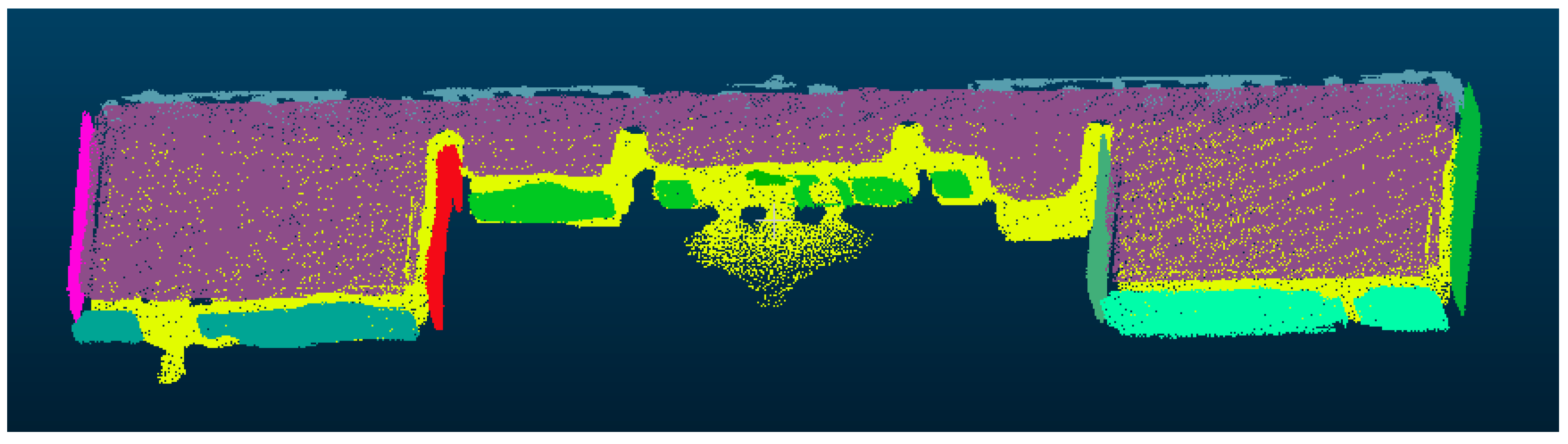
2.1.3. Plane Labelling
- XY planes
- |A| < 0.1
- |B| < 0.1
- 0.9 < |C| < 1.1
- XZ plane
- 0.9 < |A| < 1.1
- |B| < 0.1
- |C| < 0.1
- YZ planes
- |A| < 0.1
- 0.9 < |B| < 1.1
- |C| < 0.1
- /0< i < l where l is the number of segments of XY
- /0< j < n where n is the number of segments of XZ
- /0< k < m where m is the number of segments of YZ
- /0 < i < n and 0 < j < n, where n is the number of segments in XY group, results in the distance between the ith and the jth elements of the group.
2.1.4. Planes Correction
2.1.5. Wall Intersection
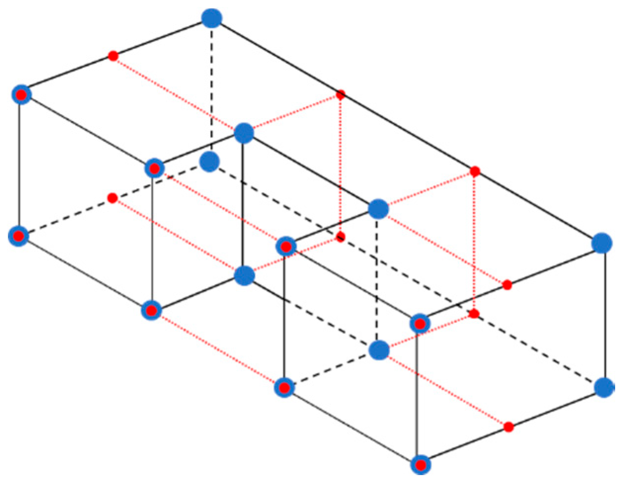
2.1.6. Vertex Estimation
2.1.7. Wall Correction
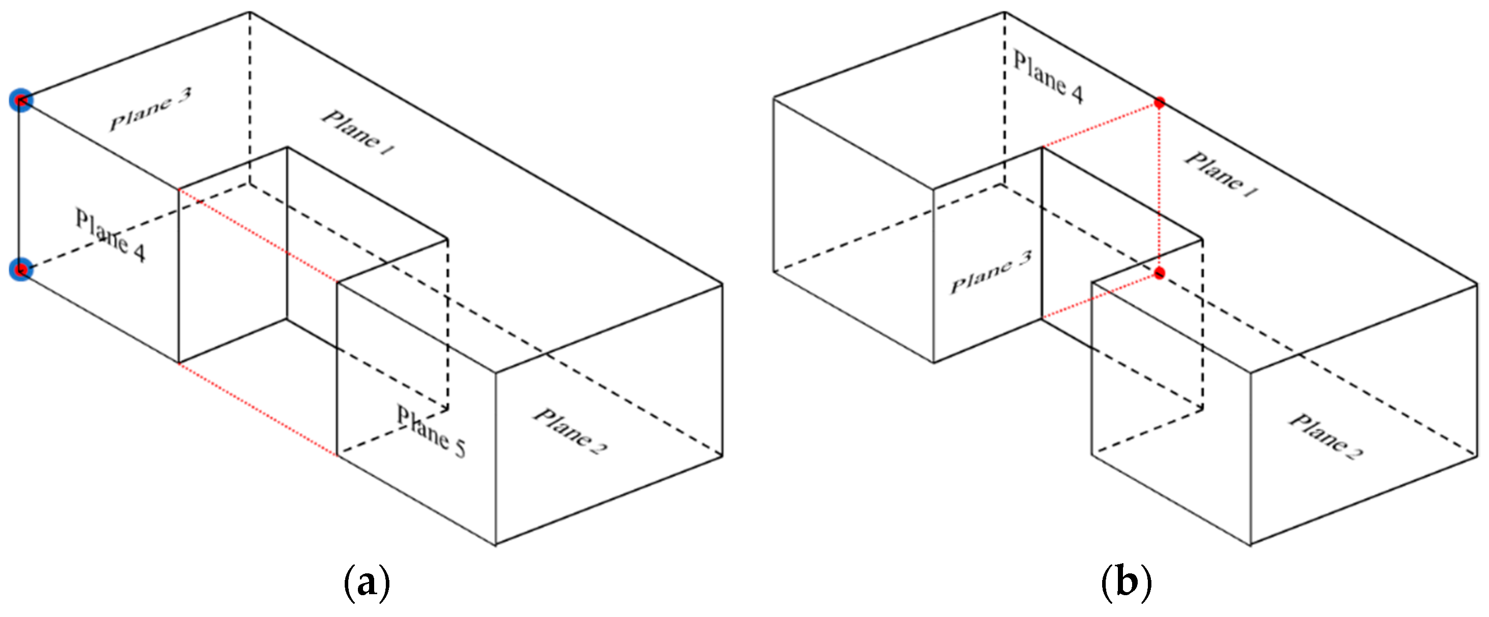
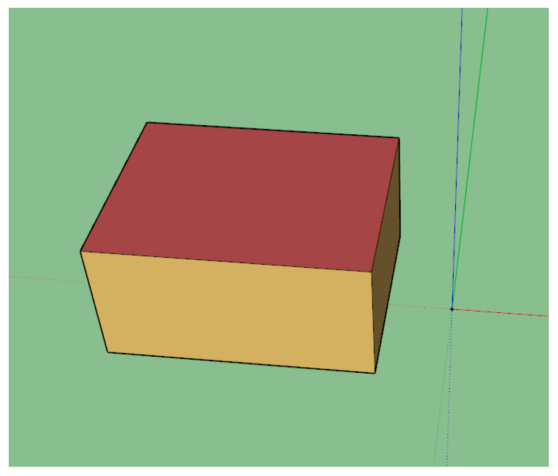
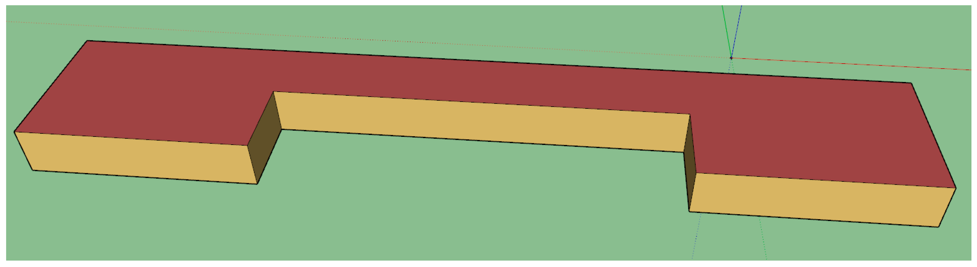
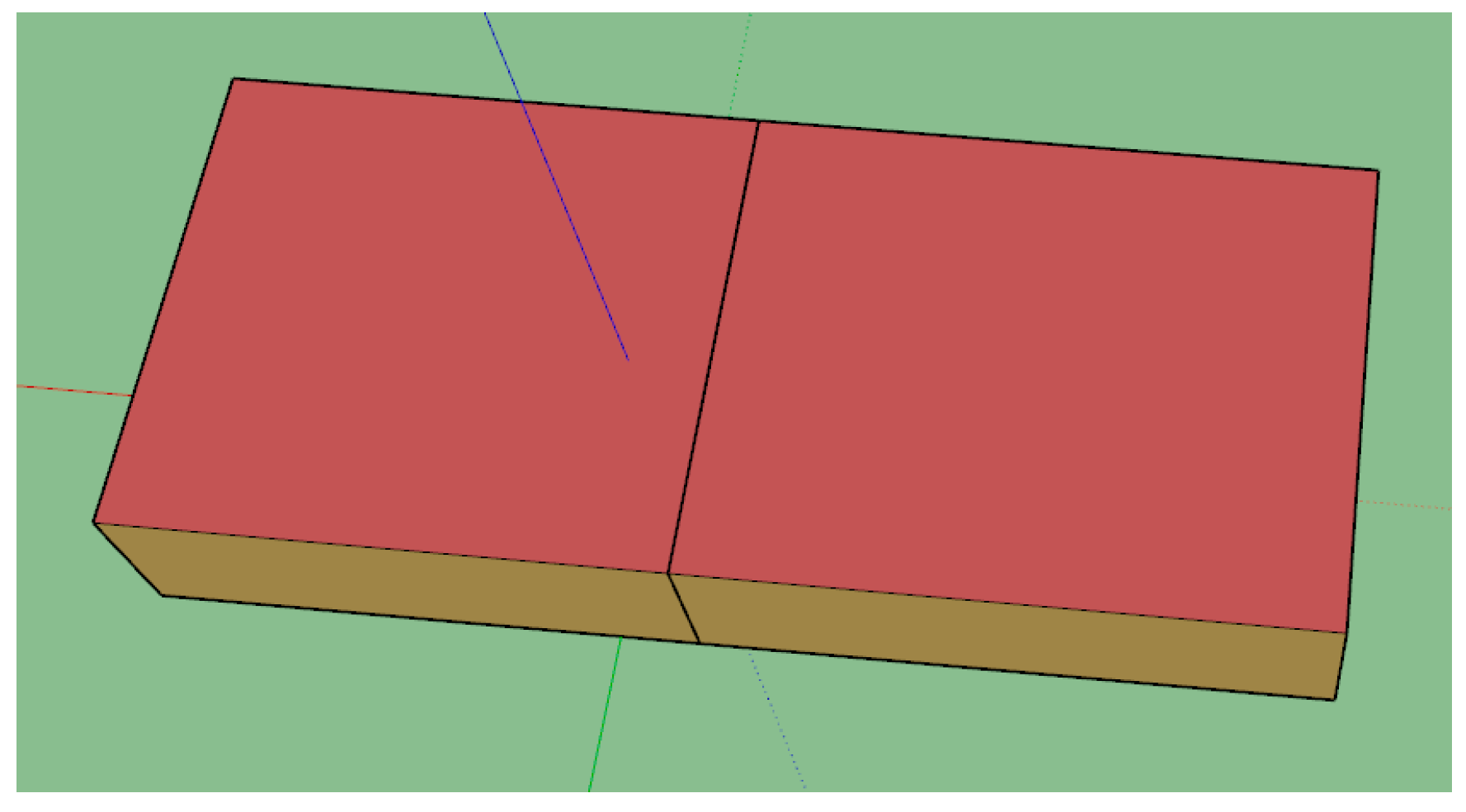
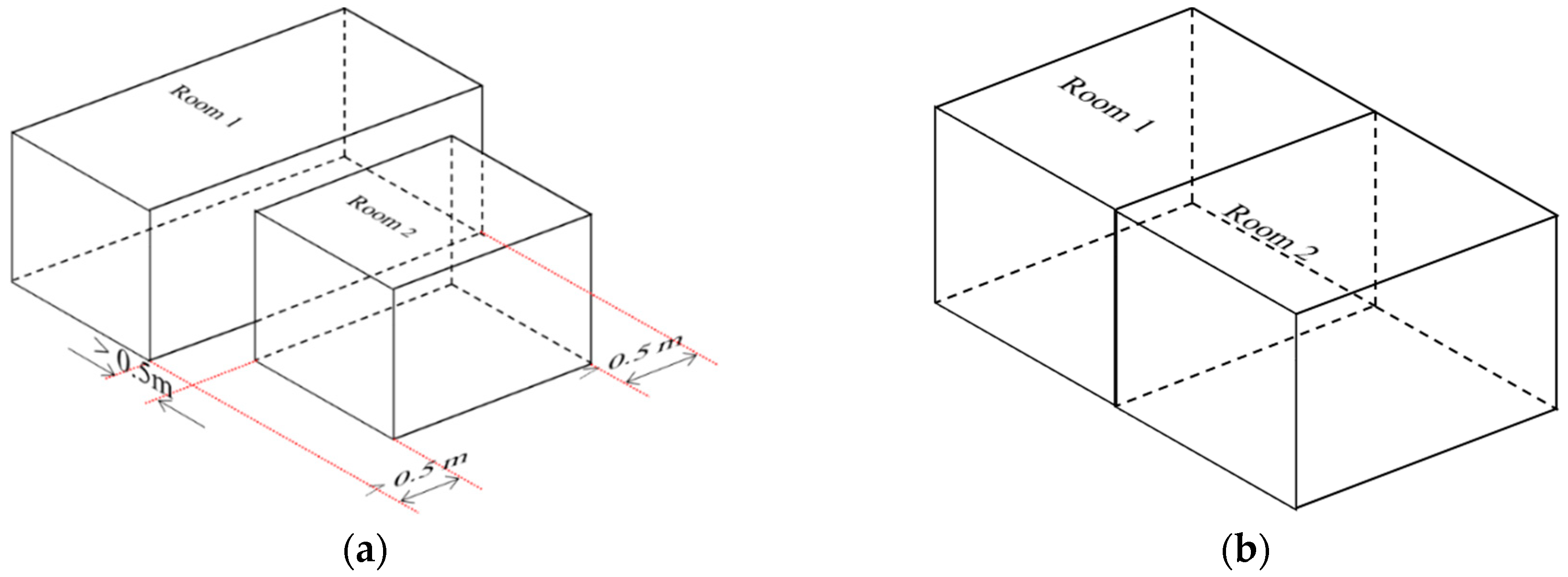
- Both polygons are equal: this is the simplest case. Only one of the polygons is required. Thus, the second is eliminated (Figure 5a).
- One polygon is contained in another but with one of the vertical edges in common: the smallest one remains without changes. The biggest one is divided into two different polygons, which correspond with the common and uncommon part (Figure 5b).
- One polygon is contained in another but without vertical edges in common. The big polygon is divided into three, one which corresponds with the common part and the other two with the uncommon parts (Figure 5c). The small polygon remains as one.
- Both polygons have in common a part of their area without being contained one in another: the two polygons are divided in a total of three, which correspond with the two uncommon areas and the common area (Figure 5d).
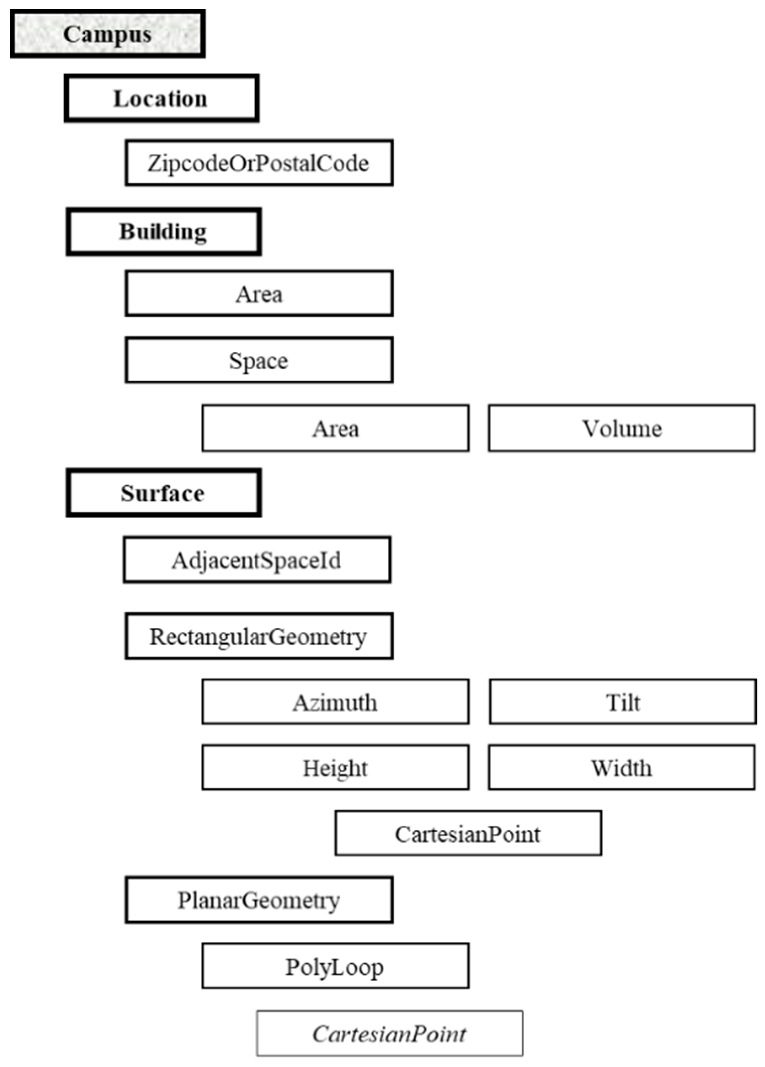
2.2. GbXML Generation.
- Campus: this node is used as base for all physical objects. It has an attribute called “id” which has the value “Campus_0” by default.
- Location: this node has a child-node called “ZipcodeOrPostalCode”. The value of this node is written by the user using the developed interface. The value is introduced in the field called “Código Zip”.
- Building: the software only writes one Building node in each gbXML file, because the analyzed point cloud belongs to only one building or to a part of it. It has two attributes: “Name”, which is introduced by the user in a field called “Nombre” and “buildingType”, which is selected by the user in a field called “Tipo”.
- Area (from building): is the summation of the area of the floors of each space of the building.
- Space: each space corresponds with one room. Each space has an attribute called “id”, which is appointed with the value <“Space” + index of the room in the data structure of the software>.
- Area (from space): area of the floor of the room. It is estimated as the area contained by the vertexes of the corresponding floor.
- Volume: volume of the room estimated as the area of the floor multiplied by the height of the ceiling.
- Surface: each surface corresponds with one wall, ceiling, or floor of the building. Each node has two attributes. The attribute “id” is set as <“Surface” + index of the surface in the data structure of the software>. The attribute “surfaceType” is set as “ExteriorWall” except for those that divide adjacent rooms; in which case they are set as “InteriorWall”, “Roof” or “SlabOnGrade” depending if the surface is a wall, a ceiling or a floor.
- AdjacentSpaceId: each surface has as much “AdjacentSpaceId” as spaces to which the surface belongs. Their value is the “id” of the corresponding space.
- RectangularGeometry: this child-node from each surface defines the overall geometry of the surface.
- Azimuth: the value of this node is estimated based on the value introduced by the user, using the interface, in a field called “Azimut”. This value is the reference value of azimuth for the Y-axis, which has the relative value of 0º. Therefore, walls with normal vector coincident to the positive X-axis have 90º, and 270º if the normal vector is coincident with the negative X-axis. Walls with normal vector coincident with negative Y-axis have azimuth equal to 270º. Azimuth 0º is assigned to horizontal slabs. The relative value is added to the reference value to estimate the azimuth of each surface.
- Tilt: assuming Manhattan World, the value of the child-node “tilt” from “RectangularGeometry” is 0º for horizontal planes and 90º for vertical planes.
- Height: this child-node from “RectangularGeometry” is estimated as the absolute value of the difference between minimum and maximum z value of each wall, except for horizontal surfaces, where height is the absolute value of the difference between the minimum and maximum y.
- Width: this child-node from “RectangularGeometry” is estimated as the area of the surface divided by the height.
- Cartesian point: this child-node from “RectangularGeometry” corresponds with the second point of the list of points for each surface.
- PlanarGeometry: this child-node from “Surface” defines the geometry of the surface.
- PolyLoop: list of the vertexes of the surface ordered counterclockwise.
- CartesianPoint: this child-node from “PolyLoop” corresponds with each vertex of the surface.
- Coordinate: this node corresponds with each coordinate of the point.
3. gbXML Results and Energy Applications
3.1. Case Studies
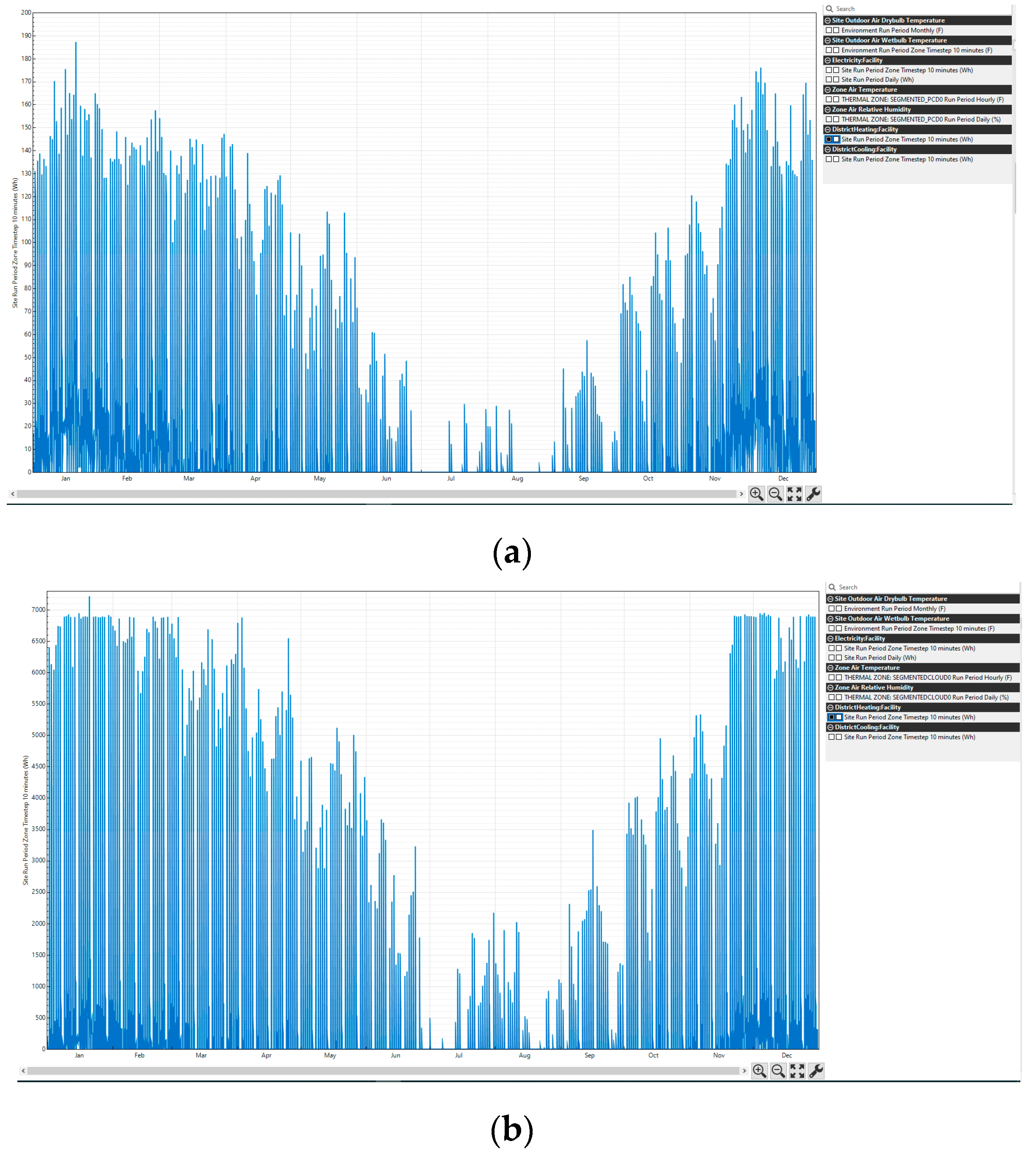
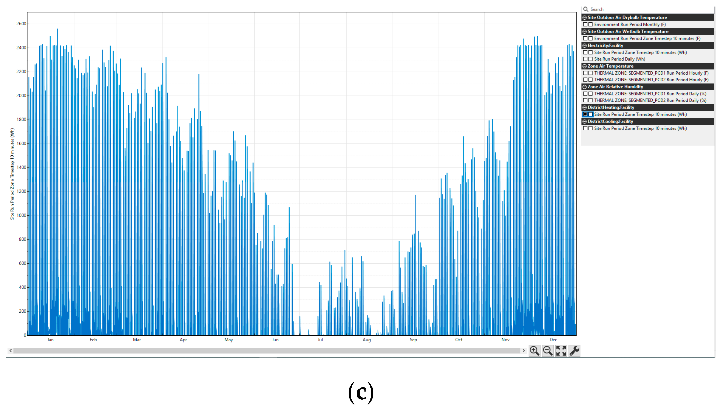
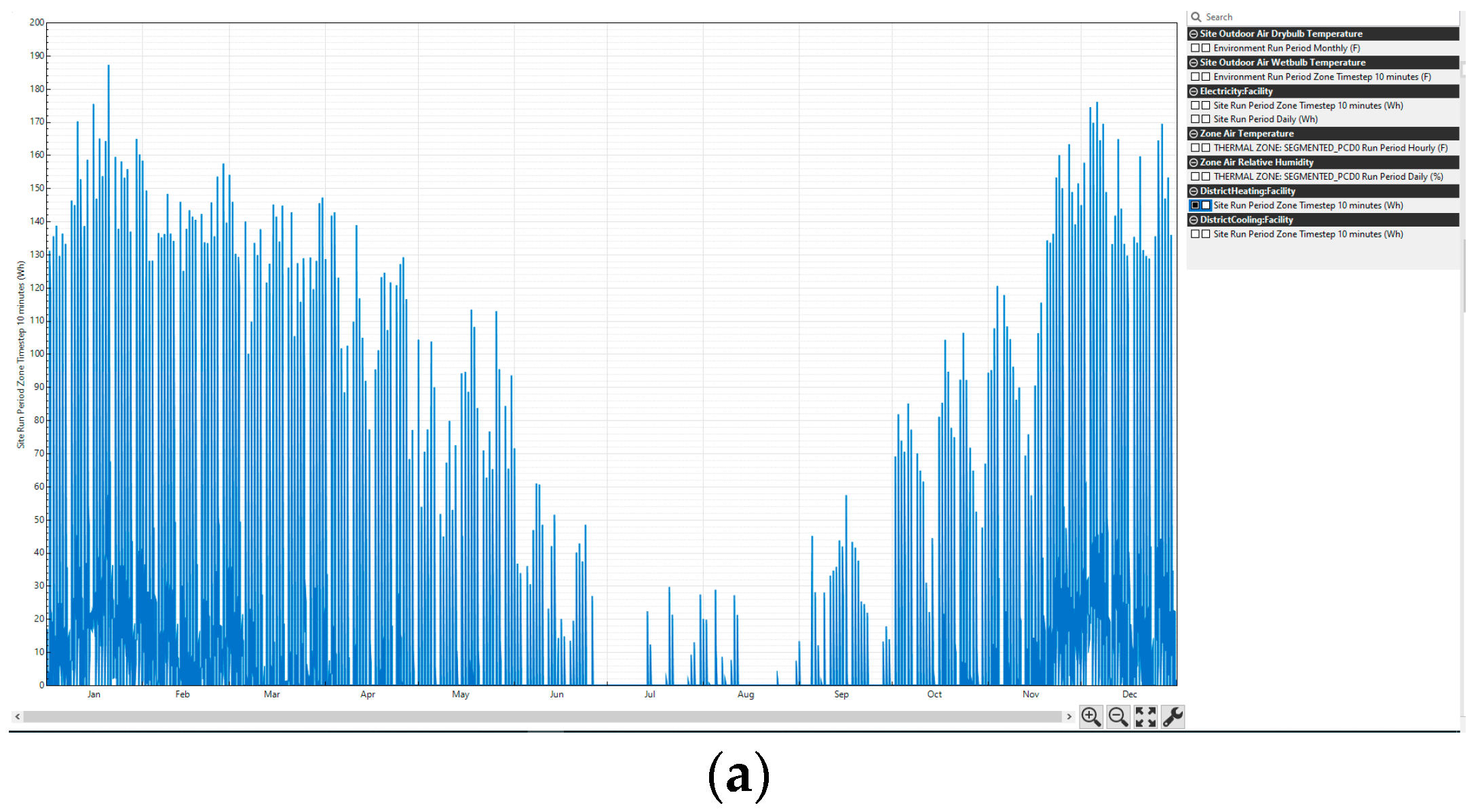
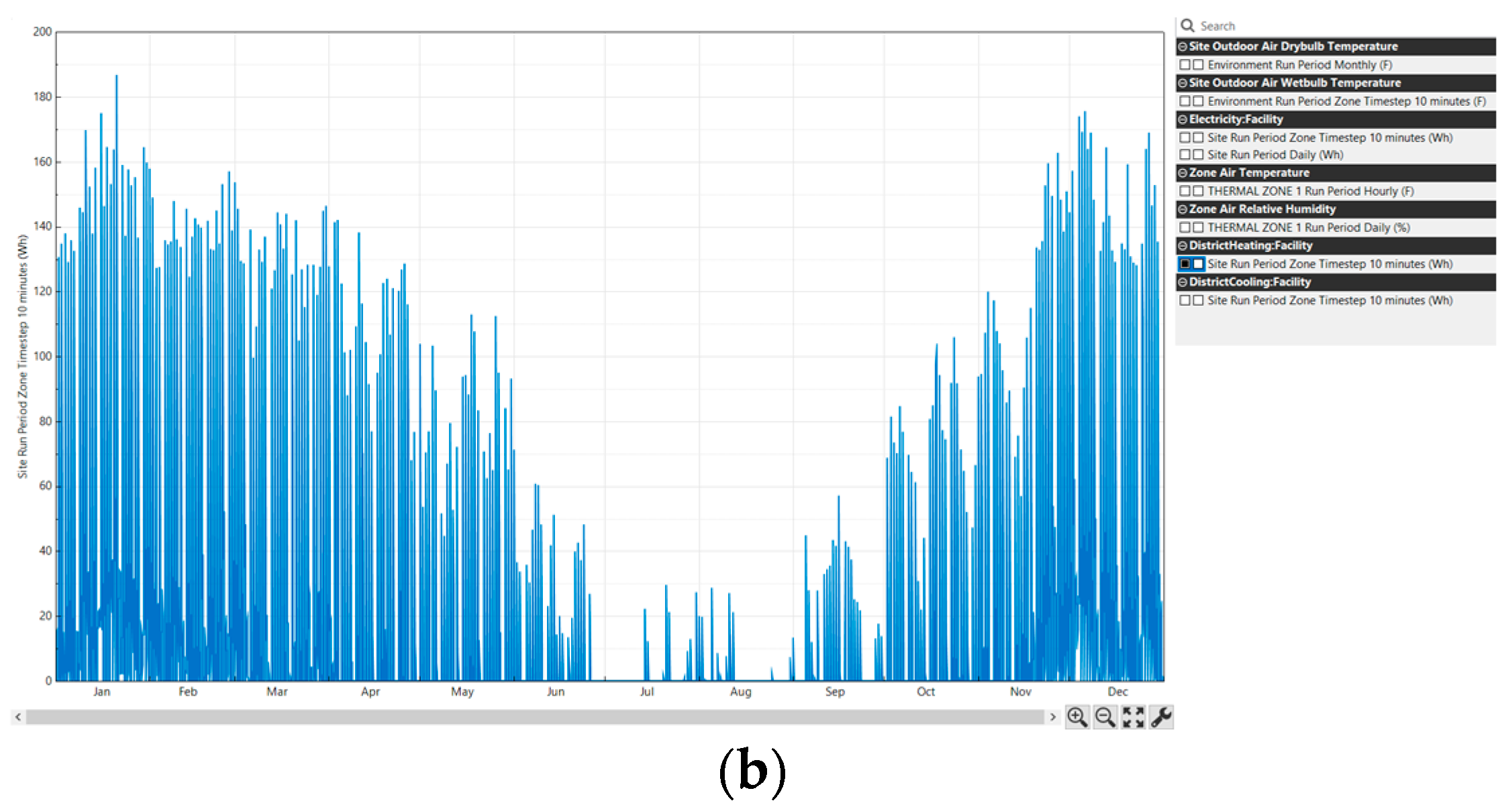
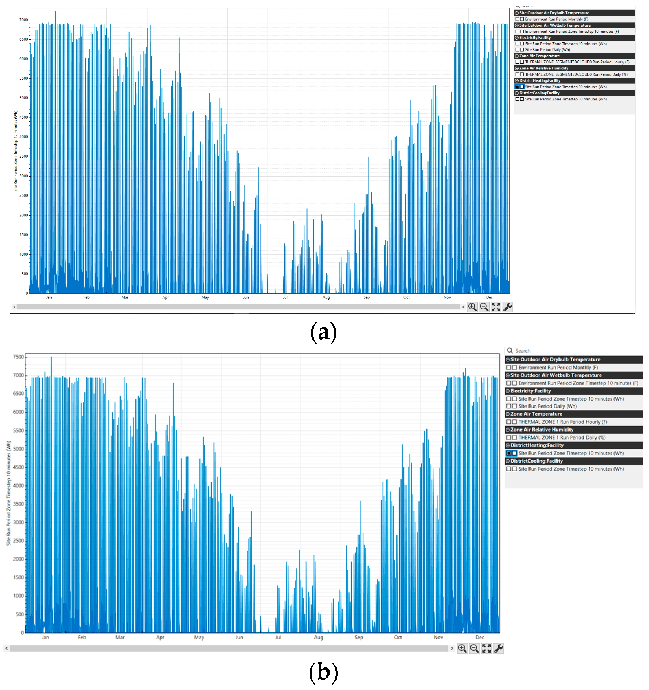
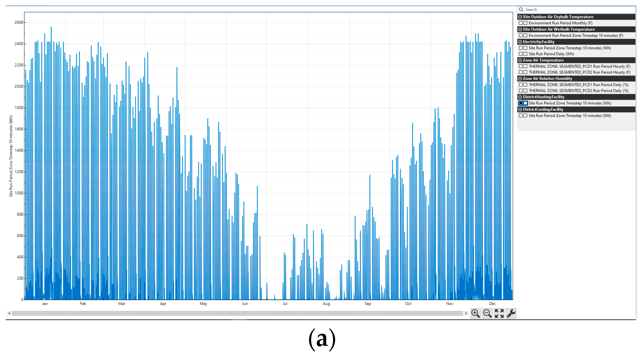
3.2. Energy Application Example
4. Discussion
4.1. Analysis of Performance of the gbXML Generation Method
4.2. Comparison of the Proposed Method with Existing Methods
5. Conclusions
Author Contributions
Funding
Acknowledgments
Conflicts of Interest
References
- EUR-Lex - 02012L0027-20200101 - EN - EUR-Lex. Available online: https://eur-lex.europa.eu/legal-content/EN/TXT/?uri=CELEX:02012L0027-20200101 (accessed on 10 June 2020).
- EUR-Lex - 31993L0076 - EN - EUR-Lex. Available online: https://eur-lex.europa.eu/legal-content/EN/TXT/?uri=uriserv:OJ.L_.1993.237.01.0028.01.ENG (accessed on 10 June 2020).
- Plan Nacional Integrado de Energía y Clima (PNIEC) 2021-2030|IDAE. Available online: https://www.idae.es/informacion-y-publicaciones/plan-nacional-integrado-de-energia-y-clima-pniec-2021-2030 (accessed on 6 July 2020).
- Tang, P.; Huber, D.; Akinci, B.; Lipman, R.; Lytle, A. Automatic reconstruction of as-built building information models from laser-scanned point clouds: A review of related techniques. Autom. Constr. 2010, 19, 829–843. [Google Scholar] [CrossRef]
- Leica Pegasus:Backpack Wearable Mobile Mapping Solution|Leica Geosystems. Available online: https://leica-geosystems.com/products/mobile-sensor-platforms/capture-platforms/leica-pegasus-backpack (accessed on 24 October 2018).
- Vexcel Imaging - Home of the UltraCam. Available online: https://www.vexcel-imaging.com/ (accessed on 23 October 2018).
- Ambrus, R.; Claici, S.; Wendt, A. Automatic Room Segmentation From Unstructured 3-D Data of Indoor Environments. IEEE Robot. Autom. Lett. 2017, 2, 749–756. [Google Scholar] [CrossRef]
- Wang, R.; Xie, L.; Chen, D. Modeling indoor spaces using decomposition and reconstruction of structural elements. Photogramm. Eng. Remote Sens. 2017, 83, 827–841. [Google Scholar] [CrossRef]
- Macher, H.; Landes, T.; Grussenmeyer, P. From Point Clouds to Building Information Models: 3D Semi-Automatic Reconstruction of Indoors of Existing Buildings. Appl. Sci. 2017, 7, 1030. [Google Scholar] [CrossRef]
- Murali, S.; Speciale, P.; Oswald, M.R.; Pollefeys, M. Indoor Scan2BIM: Building information models of house interiors. In Proceedings of the 2017 IEEE/RSJ International Conference on Intelligent Robots and Systems (IROS), Vancouver, BC, Canada, 24–28 September 2017; pp. 6126–6133. [Google Scholar]
- Ochmann, S.; Vock, R.; Klein, R. Automatic reconstruction of fully volumetric 3D building models from oriented point clouds. ISPRS J. Photogramm. Remote Sens. 2019, 151, 251–262. [Google Scholar] [CrossRef]
- Wang, Q.; Gao, J.; Li, X. Weakly Supervised Adversarial Domain Adaptation for Semantic Segmentation in Urban Scenes. IEEE Trans. Image Process. 2019, 28, 4376–4386. [Google Scholar] [CrossRef] [PubMed]
- Peng, X.; Zhu, H.; Feng, J.; Shen, C.; Zhang, H.; Zhou, J.T. Deep Clustering With Sample-Assignment Invariance Prior. IEEE Trans. Neural Netw. Learn. Syst. 2019, 1–12. [Google Scholar] [CrossRef] [PubMed]
- Peng, X.; Feng, J.; Xiao, S.; Yau, W.Y.; Zhou, J.T.; Yang, S. Structured autoencoders for subspace clustering. IEEE Trans. Image Process. 2018, 27, 5076–5086. [Google Scholar] [CrossRef] [PubMed]
- Wang, Q.; Chen, M.; Nie, F.; Li, X. Detecting Coherent Groups in Crowd Scenes by Multiview Clustering. IEEE Trans. Pattern Anal. Mach. Intell. 2020, 42, 46–58. [Google Scholar] [CrossRef] [PubMed]
- Jalaei, F.; Jrade, A. Integrating Building Information Modeling (BIM) and Energy Analysis Tools with Green Building Certification System to Conceptually Design Sustainable Buildings. ITcon 2014, 19, 494–519. [Google Scholar]
- Di Giuda, G.M.; Villa, V.; Piantanida, P. BIM and energy efficient retrofitting in school buildings. Energy Procedia 2015, 78, 1045–1050. [Google Scholar] [CrossRef][Green Version]
- Eleftheriadis, S.; Mumovic, D.; Greening, P. Renewable and Sustainable Energy Reviews; Elsevier Ltd.: Amsterdam, The Netherlands, 2017; pp. 811–825. [Google Scholar]
- GhaffarianHoseini, A.; Zhang, T.; Nwadigo, O.; GhaffarianHoseini, A.; Naismith, N.; Tookey, J.; Raahemifar, K. Application of nD BIM Integrated Knowledge-based Building Management System (BIM-IKBMS) for inspecting post-construction energy efficiency. Renew. Sustain. Energy Rev. 2017, 72, 935–949. [Google Scholar] [CrossRef]
- Wang, C.; Cho, Y.K. Automated gbXML-Based Building Model Creation for Thermal Building Simulation. In Proceedings of the 2nd International Conference on 3D Vision, Tokyo, Japan, 8–11 December 2014; pp. 111–117. [Google Scholar]
- Ham, Y.; Golparvar-Fard, M. Mapping actual thermal properties to building elements in gbXML-based BIM for reliable building energy performance modeling. Autom. Constr. 2015, 49, 214–224. [Google Scholar] [CrossRef]
- Kim, H.; Shen, Z.; Kim, I.; Kim, K.; Stumpf, A.; Yu, J. BIM IFC information mapping to building energy analysis (BEA) model with manually extended material information. Autom. Constr. 2016, 68, 183–193. [Google Scholar] [CrossRef]
- Díaz-Vilariño, L.; Lagüela, S.; Armesto, J.; Arias, P. Semantic as-built 3d models including shades for the evaluation of solar influence on buildings. Sol. Energy 2013, 92, 269–279. [Google Scholar] [CrossRef]
- IFC Schema Specifications - buildingSMART Technical. Available online: https://technical.buildingsmart.org/standards/ifc/ifc-schema-specifications/ (accessed on 12 June 2020).
- gbXML—An Industry Supported Standard for Storing and Sharing Building Properties between 3D Architectural and Engineering Analysis Software. Available online: https://www.gbxml.org/ (accessed on 13 April 2020).
- GreenBuildingXML_Ver6.01. Available online: https://www.gbxml.org/schema_doc/6.01/GreenBuildingXML_Ver6.01.html#Link19D (accessed on 18 June 2020).
- Documentation—Point Cloud Library (PCL). Available online: http://pointclouds.org/documentation/tutorials/region_growing_segmentation.php#region-growing-segmentation (accessed on 2 May 2019).
- Documentation—Point Cloud Library (PCL). Available online: http://pointclouds.org/documentation/tutorials/planar_segmentation.php#planar-segmentation (accessed on 11 February 2020).
- Tran, H.; Khoshelham, K. ISPRS Annals of the Photogrammetry, Remote Sensing and Spatial Information Sciences; Copernicus GmbH: Göttingen, Germany, 2019; pp. 299–306. [Google Scholar]
- Green Building XML (gbXML) Geometry Test Cases—Test Case 6. Available online: https://www.gbxml.org/TestCase6_Geometry.html (accessed on 31 March 2020).
- Qt XML C++ Classes|Qt XML 5.15.0. Available online: https://doc.qt.io/qt-5/qtxml-module.html (accessed on 12 June 2020).
- ZEB-REVO - geoslam. Available online: https://geoslam.com/zeb-revo/ (accessed on 5 December 2018).
- OpenStudio|OpenStudio. Available online: https://www.openstudio.net/ (accessed on 12 February 2020).
- ZEB Revo - GeoSLAM. Available online: https://geoslam.com/solutions/zeb-revo/ (accessed on 11 February 2020).


| 3D Reconstruction | Multiple Rooms | Multiple Floors | Non-Manhattan World | Fully Automatic | |
|---|---|---|---|---|---|
| Ambrus et al. [8] | x | x | x | ||
| Wang et al. [9] | x | x | x | ||
| Macher, H. et al. [10] | x | x | x | ||
| Murali et al. [11] | x | x | x | ||
| Ochmann et al. [12] | x | x | x | x | x |
| Proposed system | x | x |
| Area (m2) | Volume (m3) | Max. Consumption (Wh) | Mean Consumption (Wh) | Max Consumption/Volume (Wh/m3) | Mean Consumption/Volume (Wh/m3) | |
|---|---|---|---|---|---|---|
| Scenario 1 | 15.15 | 32.58 | 184.97 | 8.05 | 5.68 | 0.25 |
| Scenario 2 | 534.61 | 1978.06 | 7134.26 | 138.51 | 3.61 | 0.07 |
| Scenario 3 | 213.57 | 691.96 | 2531.50 | 50.02 | 3.66 | 0.07 |
| Room Segment * | Plane Segment * | Plane Label * | Wall Intersect * | Wall Correct * | gbXML Generation * | Process with User Interactions * | ||
|---|---|---|---|---|---|---|---|---|
| Scene 1 | 27 | 6 | 10 | 0 | 0 | 0 | 94 | |
| Scene 2 | 110 | 25 | 42 | 1 | 0 | 0 | 407 | |
| Scene 3 | Room 1 | 86 | 19 | 38 | 0 | 0 | 0 | 427 |
| Room 2 | 29 | 54 | 0 | 0 | 0 |
| Measured Value (m2) | Estimated Value (m2) | Absolute Error (m2) | Relative Error (%) | ||
|---|---|---|---|---|---|
| Scenario 1 | 15.03 | 15.15 | 0.12 | 0.80 | |
| Scenario 2 | 537.68 | 534.61 | 3.07 | 0.57 | |
| Scenario 3 | Room 1 | 99.02 | 99.06 | 0.04 | 0.04 |
| Room 2 | 114.97 | 114.51 | 0.46 | 0.40 |
| Measured Value (m3) | Estimated Value (m3) | Absolute Error (m3) | Relative Error (%) | ||
|---|---|---|---|---|---|
| Scenario 1 | 32.32 | 32.58 | 0.26 | 0.79 | |
| Scenario 2 | 1989.43 | 1978.06 | 11.37 | 0.57 | |
| Scenario 3 | Room 1 | 323.58 | 320.97 | 2.61 | 0.80 |
| Room 2 | 375.71 | 370.99 | 4.72 | 1.26 |
| Area (m2) | Volume (m3) | Max. Consumption (Wh) | Mean Consumption (Wh) | Max. Consumption/Volume (Wh/m3) | Mean Consumption/Volume (Wh/m3) | |
|---|---|---|---|---|---|---|
| Scenario 1 | 15.03 | 32.32 | 184.45 | 8.06 | 5.71 | 0.25 |
| Scenario 2 | 537.68 | 1989.43 | 7424.66 | 162.35 | 3.73 | 0.08 |
| Scenario 3 | 213.98 | 699.29 | 2720.17 | 64.10 | 3.89 | 0.09 |
© 2020 by the authors. Licensee MDPI, Basel, Switzerland. This article is an open access article distributed under the terms and conditions of the Creative Commons Attribution (CC BY) license (http://creativecommons.org/licenses/by/4.0/).
Share and Cite
Otero, R.; Frías, E.; Lagüela, S.; Arias, P. Automatic gbXML Modeling from LiDAR Data for Energy Studies. Remote Sens. 2020, 12, 2679. https://doi.org/10.3390/rs12172679
Otero R, Frías E, Lagüela S, Arias P. Automatic gbXML Modeling from LiDAR Data for Energy Studies. Remote Sensing. 2020; 12(17):2679. https://doi.org/10.3390/rs12172679
Chicago/Turabian StyleOtero, Roi, Ernesto Frías, Susana Lagüela, and Pedro Arias. 2020. "Automatic gbXML Modeling from LiDAR Data for Energy Studies" Remote Sensing 12, no. 17: 2679. https://doi.org/10.3390/rs12172679
APA StyleOtero, R., Frías, E., Lagüela, S., & Arias, P. (2020). Automatic gbXML Modeling from LiDAR Data for Energy Studies. Remote Sensing, 12(17), 2679. https://doi.org/10.3390/rs12172679