Abstract
Underwater photogrammetry has been increasingly used in coral-reef research in recent years. Habitat metrics extracted from resulting three-dimensional (3D) reconstructions can be used to examine associations between the structural complexity of the reef habitats and the distribution of reef organisms. We created simulated 3D models of bare surface structures and 3D reconstructions of coral morphologies to investigate the behavior of various habitat metrics that were extracted from both Digital Elevation Models (DEMs) and 3D mesh models. Analyzing the resulting values provided us with important insights into how these metrics would compare with one another in the characterization of coral-reef habitats. Surface complexity (i.e., reef rugosity), fractal dimension extracted from DEMs and vector dispersion obtained from 3D mesh models exhibited consistent patterns in the ranking of structural complexity among the simulated bare surfaces and coral morphologies. The vector ruggedness measure obtained from DEMs at three different resolutions of 1, 2, and 4 cm effectively captured differences in the structural complexity among different coral morphologies. Profile curvature and planform curvature, on the other hand, were better suited to capture the structural complexity derived from surface topography such as walls and overhanging ledges. Our results indicate that habitat metrics extracted from DEMs are generally suitable when characterizing a relatively large plot of a coral reef captured from an overhead planar angle, while the 3D metric of vector dispersion is suitable when characterizing a coral colony or a relatively small plot methodically captured from various angles.
1. Introduction
Underwater photogrammetry has been increasingly used in coral-reef surveys in recent years [1,2,3,4,5]. This range imaging technique estimates three-dimensional (3D) structures from sequential two-dimensional (2D) imagery captured by a single-lens camera (as opposed to a stereo camera) and offers a cost-effective approach to obtain high-resolution reconstructions of underwater habitats. Three-dimensional reconstructions of either coral colonies or reef habitats generated using photogrammetric techniques allow for non-intrusive extraction of physical and biological information, including the structural complexity of both biotic coral-reef communities and abiotic benthic features [2,6,7]. Structural metrics of habitat complexity extracted from 3D reconstructions are generally precise [8,9] and not subject to personal observational biases [10]. These high-resolution 3D models enable researchers to address new biological and ecological questions pertaining to coral demography, coral growth and responses of coral communities to disturbance [7,11,12].
Habitat metrics are important variables in coral-reef ecology as they affect the abundance and distribution of reef organisms including fishes [6,13,14]. These metrics can be extracted from a 3D model by rasterizing it onto a 2D plane and generating a 2.5-dimensional (2.5D) Digital Elevation Model (DEM). Digital Elevation Models can be processed in geographic information system (GIS) software [2] (also see Friedman et al. [15] about projection onto a 2D plane of best fit rather than a horizontal plane) or other programs that are capable of quantifying features of raster files [16]. Geographic information system software offers several tools to quantify habitat structures such as linear rugosity, surface complexity, slope, aspect, vector ruggedness measure (VRM) and curvature [2,17]. Fractal dimension, which combines information obtained at various spatial scales and describes the irregularity of an object, can also be determined either by changing the resolution of a DEM and measuring the 3D surface area at each of the resolutions [18,19] or by calculating the mean ranges in elevation values at different observational scales [20]. Each of these metrics possesses unique properties, thus it is important to examine precisely how the metrics respond to changes in the geometry of habitat to interpret 3D habitat structure properly.
While analyzing DEMs with GIS software makes extraction of habitat metrics relatively simple, the projection of a 3D model onto a 2D plane results in the 3D structure being captured from a single planar projection angle (e.g., overhead). This reduction of dimensionality can impact the ability to quantify structural properties. For example, overhanging surfaces and vertical walls may be poorly represented when obtaining habitat metrics from a DEM that is generated from a planar projection. To this end, exploring different ways to obtain habitat metrics directly from a 3D mesh model, which consists of vertices and triangulated faces (i.e., each face being composed of a set of three vertices), rather than through the use of a 2.5D DEM, can be beneficial. Three-dimensional fractal dimension can be obtained by placing a sphere at each of the vertices of a 3D mesh model and calculating the influence volume for a set of radius values of the spheres [21,22]. This volumetric fractal dimension has been previously applied to characterizing plants [23] and different coral morphologies [24]. Another method of estimating 3D fractal dimension is through a cube-counting procedure where the minimum number of cubes required to encase the entire 3D object is calculated for a set of side lengths of the cubes [25]. The capability of these fractal metrics for capturing structural complexity has yet to be comprehensively compared among multiple surface types.
Vector dispersion is another metric that can be used to measure 3D structure. R. A. Fisher [26] originally introduced the precision parameter , with its estimate k, in his equation for the probability density of points on a sphere. The reciprocal of k (i.e., 1/k) is vector dispersion [27]. This metric uses direction cosines of vectors that are normal (orthogonal) to individual planar surfaces to specify the orientations of the surfaces and estimates the vector variance as a measure of surface irregularity. It has been previously applied to coral-reef settings [19,27]. In particular, Carleton and Sammarco [27], while examining the success of settlement in corals in relation to increased structural complexity, determined that vector dispersion was the most appropriate metric of surface irregularity among those investigated in that study, as it ranged from 0 (least irregular) to 1 (most irregular), was sensitive to changes in scales and was correlated with changes in biological parameters measured by the aggregation of coral spats. While the metric of VRM extracted from DEMs shares a very similar underlying concept in quantifying the structural complexity and has been applied to coral-reef habitats [18,28,29], vector dispersion extracted from 3D mesh models has rarely been used to characterize coral-reef habitats (but see Young et al. [19]).
This study examined the behavior of different habitat metrics obtained from either DEMs or 3D mesh models using both simulated bare surface structures and 3D reconstructions of individual coral colonies with different morphologies. As the 3D structure of a coral reef is affected by both coral morphology and the underlying surface topography, the use of simulated surfaces and individual coral morphologies helps to separate their effects. We focused on six habitat metrics obtained from DEMs (surface complexity, fractal dimension, slope, VRM, profile curvature and planform curvature) and three habitat metrics obtained from 3D mesh models (volumetric fractal dimension, cube-counting fractal dimension and vector dispersion). To our knowledge, this is the first study that compared habitat metrics obtained from DEMs and those obtained from 3D mesh models and closely examined how coral morphology and surface topography individually and collectively affect these habitat metrics. Habitat metrics extracted from 3D reconstruction of coral reefs are increasingly used to examine associations between the structure of the habitat and the distribution of reef organisms [6,30,31]. Understanding differences in the behavior of these metrics in characterizing the architecture of coral-reef habitats is therefore essential for future studies in coral-reef ecology.
2. Materials and Methods
2.1. Generation of Surface Models
Simulated surface models were generated as 3D mesh models using Blender v.2.80 (Blender Foundation, Amsterdam, The Netherlands). Each model was created to have a 2D planar area of 1 × 1 m, with vertices being spaced at an approximately 0.8-cm interval, and all faces were triangulated. Blender’s proportional editing function was used with “random” falloff that was set to 0.01 m in the z (vertical) direction so that slight surface roughness was added to replicate bare reef substrata. The models imitated the following six surface structures: flat, linear slope (linear), upward convexity (convex), upward concavity (concave), vertical wall (wall) and overhanging ledge. We chose these six surface structures to examine the structural complexity of reef substrata and to compare different types of sloping surfaces with a flat surface. The wall and overhanging ledge structures were included because such structures are common in coral-reef habitats, and the sudden changes in depth that are associated with these structures would likely contrast with the gradual changes in depth associated with sloping surfaces. Comparisons between the wall and overhanging ledge structures were also of interest, as these two structures should have minimal differences in their DEMs when captured from the overhead angle, but not in their 3D mesh models, which can capture the area under an overhang. For all models, the maximum difference in z-values was set to ≈0.25 m (Figure 1).
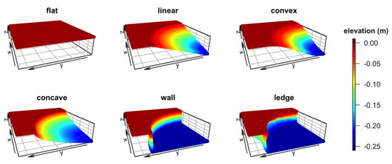
Figure 1.
Three-dimensional visualization of six different simulated surface structures: flat, slope, convex, concave, drop and overhanging ledge.
2.2. Generation of Coral Models
Images of individual coral colonies were collected from shallow-water reefs off the south shore of the island of O‘ahu, Hawai‘i. Coral species and morphologies that were modeled included branching Pocillopora meandrina, branching Porites compressa, mounding Porites lobata, and encrusting Montipora capitata. We specifically chose coral colonies of similar size (≈30 cm) to make reasonable comparisons among different morphologies. For each surveyed colony, a SCUBA diver first placed two calibrated scale bars with coded targets at opposing corners of the colony and collected overlapping imagery aiming for 70∼80% overlaps from one photograph to the next. The diver manually took each image using the single shooting setting while swimming around the colony in a spiral pattern. Images were initially collected approximately a meter away from the colony and the camera was moved progressively closer to capture small structural details. All photographs were taken using a Sony 7III full-frame camera with a 24–70 mm lens in a Nauticam housing with an 8.5-inch dome port. The focal length of 24 mm was used throughout the process of image collection, with a shutter speed of 1/250 s, an aperture of f/11 and an auto ISO.
Three-dimensional models of coral colonies were constructed from the imagery using the software Agisoft Metashape v.1.5 Professional Edition (Agisoft LLC., St. Petersburg, Russia). Camera calibration and optimization were completed using the Metashape software. The software performs calibration using Brown’s distortion model and is capable of resolving the optical characteristics of the camera lens directly from the metadata of images without prior calibration. For each model, a sparse 3D point cloud was generated through the photo-alignment process of the software. After scaling the model and optimizing the results of photo alignment based on the calibrated scale bars, a dense point cloud and a 3D mesh model were generated. The process was completed on an Intel Core i7 laptop with a 32 GB RAM and Radeon RX Vega 56 external GPU.
Three-dimensional mesh models were imported into Blender for further cleaning by removing small isolated fragments and filling any holes. Blender’s decimate modifier was used for each model to set the number of vertices to ≈62,000 and the number of faces to ≈124,000 (Figure 2). A flat surface of 0.4×0.4 m was then added to each of the four models to examine how each habitat metric would shift when a less structurally complex “substratum” was added to a more structurally complex coral colony. Similar to the flat surface of the simulated surface models, Blender’s proportional editing function was used with “random” falloff set to 0.004 m in the z direction in order to add slight surface roughness (Figure 3).
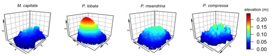
Figure 2.
Three-dimensional visualization of four coral colonies with different morphologies: encrusting M. capitata, mounding P. lobata, branching P. meandrina and branching P. compressa.
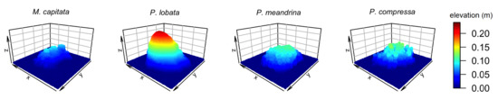
Figure 3.
Three-dimensional visualization of four coral colonies with different morphologies with a substratum: encrusting M. capitata, mounding P. lobata, branching P. meandrina and branching P. compressa.
2.3. Digital Elevation Models
Three-dimensional mesh models were exported from Blender as COLLADA (.dae) files. Digital Elevation Models were generated using ArcMap v.10.7 (Environmental Systems Resource Institute, Redlands, USA) by importing the COLLADA files into a multipatch feature class, converting them to raster of 1-cm cell size and exporting them as GeoTIFF elevation data files with local coordinates (Figure 4, Figure 5 and Figure 6). We chose to use the DEM cell size of 1 cm as previous studies that utilized the same photogrammetric technique in coral-reef environments generated reef models within a few-millimeter accuracy based on ground sampling distances and errors [2,7,18]. The use of 1-cm cell size would ensure that the resolution of DEMs is standardized and well within the range of model accuracy.
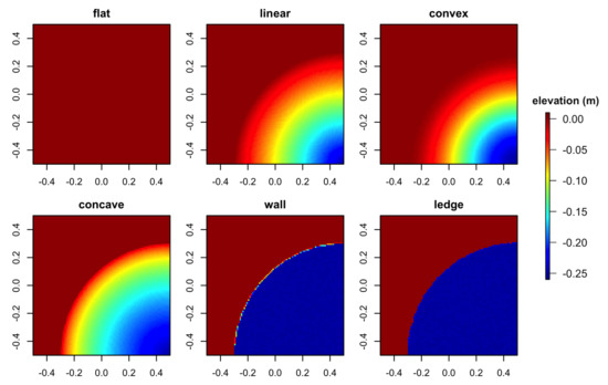
Figure 4.
Digital Elevation Models obtained from the six simulated surface structures: flat, linear, convex, concave, wall and overhanging ledge.
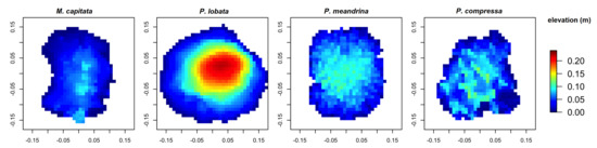
Figure 5.
Digital Elevation Models obtained from the four reconstructed coral colonies with different morphologies: encrusting M. capitata, mounding P. lobata, branching P. meandrina and branching P. compressa.
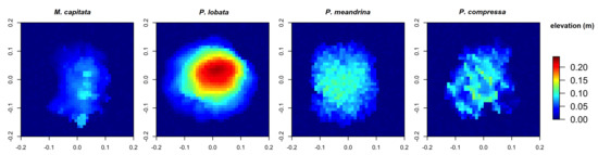
Figure 6.
Digital Elevation Models obtained from the four reconstructed coral colonies with different morphologies with a substratum: encrusting M. capitata, mounding P. lobata, branching P. meandrina and branching P. compressa.
All DEMs were processed in the statistical software R v.3.6.2 (R Core Team, 2019) to obtain habitat metrics using custom scripts written in R with sp [32,33], raster [34] and rgeos [35] packages (Data S1) following the methods of Fukunaga et al. [18]. Habitat metrics obtained from DEMs were surface complexity (the ratio of the 3D surface area along reef contours to the 2D planar area), slope [17,36], VRM [17,37] and profile and planform curvature [38]. With the exception of VRM, these metrics were obtained only at 1-cm resolution. For VRM, 2- and 4-cm resolutions were also used because VRM at these resolutions effectively captures structural differences among certain coral morphologies [28]. In addition, fractal dimension, FDDEM, was calculated as FDDEM = 2 − slope of [logS()/log()], in which was a resolution of the DEM and S() was the 3D surface area at the given resolution [19]. The resolutions used to calculate fractal dimension were 1, 2, 4 and 8 cm. For all these metrics, the resolution of 1 cm (and 2 and 4 cm for VRM) was successfully used in a previous study to capture the 3D habitat structure provided by specific benthic organisms in the 3D reconstruction of coral reefs [28]. While models used in the present study were much smaller than reef plots, which are typically tens or sometimes hundreds of square meters in size, the visualization of the DEMs at 1-cm resolution clearly showed the structural differences among either the surface structures or the coral morphologies (Figure 4, Figure 5 and Figure 6). Thus, our analysis at 1-cm resolution should adequately capture their structural differences. The upper cell size of 8 cm for FDDEM was chosen based on the planar area of the coral colony models (i.e., ≈30 cm in diameter; see Fukunaga et al. [18] for more details about choosing the upper limit of cell size for the calculation of FDDEM). Note that for surface complexity and FDDEM, each metric generated a single value per DEM, while slope, VRM and profile and planform curvature values were generated for each cell of a DEM.
2.4. 3D Mesh Models
Three-dimensional mesh models were exported from Blender as Wavefront (.obj) files and further processed to extract habitat metrics using custom scripts written in Python 3.7 (Python Software Foundation, www.python.org) with SciPy [39], NumPy [40,41] and Matplotlib [42] packages (Data S2). Habitat metrics obtained from 3D mesh models were the volumetric Bouligand-Minkowski fractal dimension, cube-counting fractal dimension and vector dispersion.
Volumetric fractal dimension was obtained by first generating a complete set of points placed at 1-cm interval along x, y and z axes in 3D space, thereby creating 1-cm cubes, and evaluating the distance from the centroid of each cube to the nearest vertex. The influence volume, V(r), of spheres of radius r placed at each vertex was estimated by counting the number of 1-cm cubes whose distance from the centroid to the nearest vertex was less than or equal to r. Volumetric fractal dimension, FDvol, is FDvol = 3 − slope of [logV(r)/log(r)] [22,23]. The maximum for r for each model was set in the scripts (Data S2) to be greater than the maximum distance between any two vertices in the 3D mesh model.
Cube-counting fractal dimension was estimated by first encasing a 3D mesh model in a smallest possible cube with a side length smax and then halving the side length to generate a set of smaller cubes and counting the number of cubes that contained vertices, C(s), at a given side length s = {smax, smax, smax, …}. Cube-counting fractal dimension, FDcube, is FDcube = slope of [logC(s)/log(1/s)] [25]. The minimum side length was set in the scripts (Data S2) to be ≥1 cm.
Vector dispersion (1/k) was calculated by obtaining all vectors normal (i.e., orthogonal) to the individual triangulated faces of the 3D mesh model, for 1/k = (i − R1) (i− 1). Here, i was the number of faces and R1 was [() + () + ()], in which , and were the direction cosine of vector normal to each of the i faces with respect to the x, y and z axes, respectively [27].
3. Results
3.1. Surface Models
Surface complexity and FDDEM extracted from the DEMs of the six simulated surface structures showed a similar pattern with a relatively large difference between the wall and overhanging ledge structures and the rest of the surface types (Figure 7a,b). The overhanging ledge structure had higher values of surface complexity and FDDEM than the wall structure (Figure 7a,b). The pronounced difference was somewhat unexpected as the only difference in the two DEMs was at the edge of the drop where the change in elevation from 0 to m was slightly more abrupt with the overhanging ledge structure than the wall structure (Figure 4). Surprisingly, FDDEM did not capture the structural changes very well from the flat surface to either the linear surface or the convex (Figure 7b) despite the increases in surface areas in both surface types captured by surface complexity (Figure 7a).
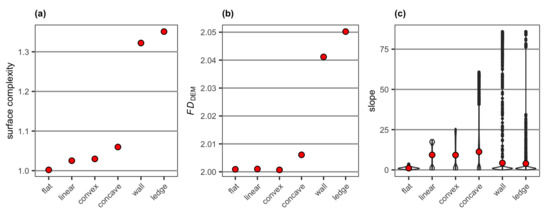
Figure 7.
Values of (a) surface complexity and (b) FDDEM and a violin plot for (c) slope extracted from the DEMs of the six simulated surface structures. Note surface complexity and FDDEM generate a single value per DEM, while slope is generated for each cell of a DEM. The mean value of slope for each surface structure is shown as red points.
The range of slope values extracted from the DEMs of the six simulated surface structures increased from the flat surface to the linear surface, convex, concave and the wall and overhanging ledge structures (Figure 7c). The mean of slope values was, however, the highest with the concave followed by the convex and linear surface (Figure 7c). Slope was steeper for the concave than the convex at the edge where the elevation started dropping from 0 m (Figure 1), and this produced more extreme values for the concave than the convex and resulted in the higher mean value (Figure 7c). The linear surface had two clumps, one close to 0 degrees for the flat part of the surface and the other one near 18 degrees for the consistently sloping (i.e., linear) surface (Figure 7c). While the wall and overhanging ledge structures contained higher slope values than all other surface types, most areas of these structures were flat (i.e., both at the top and the bottom of the wall/ledge), resulting in the lower mean slope values than the three sloping surfaces (Figure 7c).
An overall pattern of the mean VRM values obtained from the DEMs of the six simulated surface structures was similar for the three different resolutions at which this metric was obtained; they increased from the flat surface to the convex and linear surface, then to the concave and finally to the wall and overhanging ledge structures (Figure 8). There was very little difference among the flat and linear surfaces and convex for VRM obtained at 1-cm resolution (Figure 8a). For each surface structure, the mean value gradually increased from the higher resolution of 1 cm to the lower resolution of 4 cm, and the 4-cm resolution best separated the differences in the structural complexity among the six surface structures, which all had the size of 1 m with the maximum elevation change of 0.25 m.
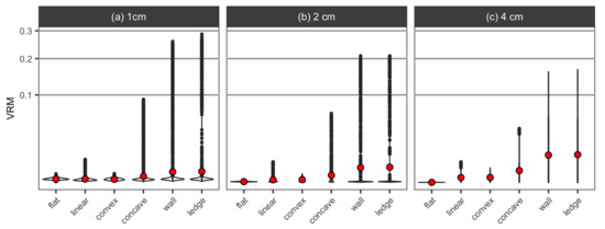
Figure 8.
Violin plots for VRM extracted at three different resolutions, (a) 1 cm, (b) 2 cm and (c) 4 cm, from the DEMs of the six simulated surface structures. The mean value of VRM for each surface structure is shown as red points.
Curvature values obtained from the DEMs of the six simulated surface structures were mostly close to 0 (i.e., flat) and within the range of ±25, with the exception of extreme values (i.e., outliers) found with the wall and overhanging ledge structures (Figure 9). As curvature metrics measure the rate of change in the gradient and direction of slope, the sudden changes in depth with the wall and overhanging ledge structures resulted in these extreme positive and negative values. For both profile and planform curvature, mean values were positive and close to 0 for the flat and linear surfaces, convex and concave. The wall structure had higher mean values for both curvature types than these surface structures, while the overhanging ledge structure had negative mean values for both types of curvature (Figure 9b).
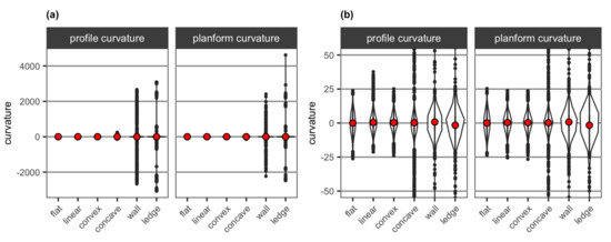
Figure 9.
Violin plots for profile curvature and planform curvature extracted from the DEMs of the six simulated surface structures (a) for the entire data range and (b) for the range between and 50. The mean value of curvature for each surface structure is shown as red points.
Vector dispersion and FDvol obtained from the 3D mesh models of the six simulated surface structures showed a pattern similar to surface complexity and FDDEM obtained from the DEMs, with the values increasing from the flat surface to linear surface, convex and concave, then to the wall and overhanging ledge structures (Figure 10). Vector dispersion separated the wall and overhanging ledge structures from all other surface structures more clearly than FDvol. FDcube had, on the other hand, a different pattern, in which the linear surface and convex had lower values than the flat surface, and the concave and wall structure were not well separated (Figure 10a).
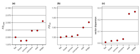
Figure 10.
Values of (a) FDcube, (b) FDvol and (c) vector dispersion extracted from the 3D mesh models of the six simulated surface structures.
3.2. Coral Models
Surface complexity and FDDEM extracted from the DEMs of four reconstructed coral colonies showed a similar pattern, with branching P. compressa having the highest value followed by branching P. meandrina, mounding P. lobata and encrusting M. capitata (Figure 11a,b). On the other hand, the range of slope values for the four colonies were all between 0 and 80 degrees (Figure 11c). The mean slope value was the highest for mounding P. lobata having slope values between 30 and 80 degrees for most of the DEM cells, followed by branching P. compressa, branching P. meandrina and encrusting M. capitata. Adding a flat surface to each of the coral colonies resulted in overall decreases in surface complexity and FDDEM (Figure 11d,e). The mean slope values also decreased as they were influenced by the near-zero values derived from the flat surface (Figure 11f).
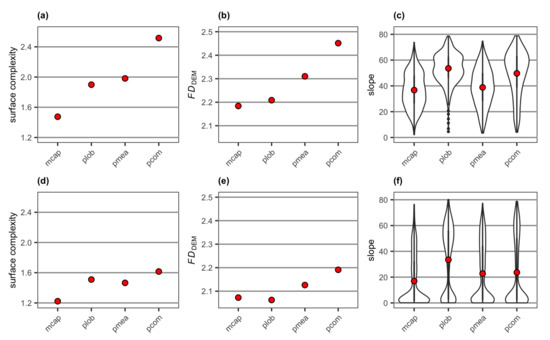
Figure 11.
Values of (a) surface complexity and (b) FDDEM and a violin plot for (c) slope extracted from the DEMs of the four reconstructed coral colonies with different morphologies, and values of (d) surface complexity and (e) FDDEM and a violin plot for (f) slope extracted from DEMs of the four reconstructed coral colonies with different morphologies with a substratum: mcap = encrusting M. capitata, plob = mounding P. lobata, pmea = branching P. meandrina and pcom = branching P. compressa. Note surface complexity and FDDEM generate a single value per DEM, while slope is generated for each cell of a DEM. The mean value of slope for each colony is shown as red points.
The mean VRM values obtained from the DEMs of the four reconstructed coral colonies at 1-cm resolution were the highest for branching P. compressa, followed by branching P. meandrina, encrusting M. capitata and mounding P. lobata (Figure 12a). At 2-cm resolution, the mean VRM values decreased for the two branching species and increased for encrusting M. capitata and mounding P. lobata (Figure 12a). The coral colonies were too small to obtain VRM at 4-cm resolution. For both 1- and 2-cm resolutions, adding a flat surface to each colony resulted in an increase in the upper range of VRM values for all coral morphologies (Figure 12b), which was probably due to the presence of the coral-substratum interface in the models as VRM measures dispersion in the surface directions. The flat surface also added cells with VRM values close to zero, which was more apparent at 1-cm resolution and resulted in a reduction in the mean VRM values for all coral morphologies. At 4-cm resolution, mounding P. lobata had the highest value of mean VRM, followed by the two branching corals and encrusting M. capitata (Figure 12b).
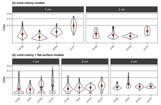
Figure 12.
Violin plots for (a) VRM extracted at two different resolutions, 1 cm and 2 cm, from the DEMs of the four reconstructed coral colonies with different morphologies, and (b) VRM extracted at three different resolutions, 1 cm, 2 cm and 4 cm, from the DEMs of the four reconstructed colonies with different morphologies with a substratum: mcap = encrusting M. capitata, plob = mounding P. lobata, pmea = branching P. meandrina and pcom = branching P. compressa. The mean value of VRM for each colony is shown as red points. The coral colonies were too small to obtain VRM at 4-cm resolution.
The range of curvature values obtained from the DEMs of the four reconstructed coral colonies increased from less structurally complex encrusting and mounding morphologies to more structurally complex branching morphology (Figure 13a). There were also more cells with values close to 0 (i.e., flat) for encrusting M. capitata and mounding P. lobata than the two branching corals (Figure 13a), likely resulting from these two less structurally complex morphologies having more smooth surface area. The mean profile curvature values were positive (i.e., upwardly convex) for all coral morphologies, while the mean planform curvature values were negative (i.e., laterally convex). Adding a flat surface to each colony increased the range of curvature values for each coral (Figure 13b), likely resulting from the presence of the coral-substratum interface where abrupt changes in slope occurred. Adding a flat surface also resulted in the mean profile curvature values turning negative (i.e., upwardly concave), likely again due to the presence of the coral-substratum interface, whereas the mean planform curvature values remained negative (i.e., laterally convex).
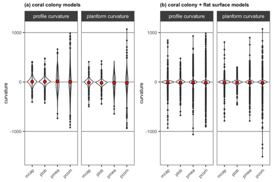
Figure 13.
Violin plots for profile curvature and planform curvature extracted from the DEMs of (a) the four reconstructed coral colonies with different morphologies and (b) the four reconstructed coral colonies with different morphologies with a substratum: mcap = encrusting M. capitata, plob = mounding P. lobata, pmea = branching P. meandrina and pcom = branching P. compressa. The mean value of curvature for each colony is shown as red points.
Vector dispersion, FDcube and FDvol obtained from the 3D mesh models of the four reconstructed coral colonies showed increases in the values from encrusting M. capitata to mounding P. lobata, branching P. meandrina and branching P. compressa (Figure 14a–c), which was similar to the pattern observed with surface complexity and FDDEM obtained from the DEMs. Adding a flat surface to each colony decreased vector dispersion values (Figure 14f). This was not the case for either FDcube or FDvol; their values increased for encrusting M. capitata and mounding P. lobata and decreased for the two branching corals (Figure 14d,e). The ranking of structural complexity measured by FDvol was preserved after the addition of a flat surface to each coral colony (Figure 14b,e), while FDcube was the highest for mounding P. lobata with an added flat surface (Figure 14d).
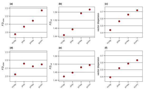
Figure 14.
Values of (a) FDcube, (b) FDvol and (c) vector dispersion extracted from the 3D mesh models of the four reconstructed coral colonies with different morphologies, and (d) FDcube, (e) FDvol and (f) vector dispersion extracted from the 3D mesh models of the four reconstructed coral colonies with different morphologies with a substratum: mcap = encrusting M. capitata, plob = mounding P. lobata, pmea = branching P. meandrina and pcom = branching P. compressa.
4. Discussion
The present study examined the behavior of multiple habitat metrics extracted from 2.5D DEMs and 3D mesh models using simulated bare surface structures and reconstructed coral colonies. Associations between habitat metrics extracted from DEMs, including surface complexity, fractal dimension, mean slope, mean VRM and mean profile and planform curvature, have been previously examined using 3D reconstruction of coral reefs in the Northwestern Hawaiian Islands [18]. The present study utilized those structural metrics and was specifically designed to examine how certain coral morphologies and topographic features would affect each specific habitat metric. It is also the first study that directly utilized vertices and faces of 3D mesh models to obtain true 3D metrics to measure the structural complexity of coral-reef habitats.
In the previous study that examined associations between habitat metrics extracted from DEMs, metrics of structural complexity were found to be highly correlated with one another [18]. The present study further confirmed the similarity between surface complexity and FDDEM. The ranking of structural complexity measured by these metrics was mostly consistent for the six simulated surface structures and the four reconstructed coral colonies with different morphologies (with or without a flat surface). Surface complexity computed as the ratio of 3D surface area to the 2D planar area is analogous to reef rugosity measured by the classic chain-and-tape method [43] and easily interpretable. FDDEM looks at the rate of changes in the 3D surface area across different resolutions. The similarity of surface complexity and FDDEM is likely due to the calculations of both metrics being based on 3D surface areas. Despite their overall similarity, however, FDDEM did not effectively capture the structural change from the flat surface to either the linear surface or the convex in comparison to surface complexity (Figure 7a,b). This is likely due to the nature of fractal dimension metrics that captures the “irregularity” of an object. The linear surface and convex had very smooth gradual slope, whereas the concave had a more abrupt change in elevation at the edge of the transition from flat to sloping (Figure 1), which resulted in the higher FDDEM value than the flat and linear surfaces and the convex. Smooth sloping surfaces do not create irregularity in the way that sudden changes in elevation or the presence of benthic organisms, such as corals, or abiotic features do and are also less likely to be ecologically important in terms of providing shelters or microhabitats. Thus, this property of FDDEM can be advantageous when being used in ecological studies. FDDEM has also been previously shown to capture the structural complexity of sessile reef organisms better than surface complexity, potentially due to its multiscale nature [28], thus it is a more suitable metric for use in ecological studies of coral reefs.
Unlike either surface complexity or FDDEM, slope is the measure of steepness and is calculated for each cell of a DEM based on the surface properties of 3×3 neighboring cells [17]. The present study clearly demonstrated how mean slope, which was obtained by averaging slope values in all the cells of a DEM, can exhibit different responses to habitat complexity in comparison with the other metrics used in this study. Our results also suggest that the use of mean slope as a metric of structural complexity requires some caution as extremely large slope values generated in some cells by the grades created by a 3D structure can be canceled out when there are a large number of cells with relatively low slope values (e.g., the wall and overhanging ledge structures in Figure 7c). Utilizing the average value of slope to characterize reef structures may result in a misleading representation of the structural complexity occurring within a given coral reef habitat.
Vector ruggedness measure (VRM) quantifies the variability in the direction where each surface is facing based on a combination of slope and aspect metrics obtained from 3 × 3 neighboring cells of a DEM [37]. It has been previously shown to be resolution specific, with the structural complexity of branching corals being captured at relatively high resolutions (e.g., 1 cm), encrusting corals at intermediate resolutions, and mounding corals at relatively low resolutions of 4 to 16 cm [28]. In the present study, this response of VRM to changes in DEM resolution was particularly apparent with the coral models with a flat surface where the mean VRM was the highest for the two branching corals at 1-cm resolution and for the mounding P. lobata at 4-cm resolution. The simulated surface structures, whose planar areas were 1 m with a maximum elevation change of 0.25 m, were also best separated at 4-cm resolution. This suggests that VRM obtained at cell sizes larger than 4 cm could effectively capture large-scale structural complexity arising from the surface topography of a reef that is independent of live benthic cover. This approach may not be practical in coral-reef applications as a wide range of resolutions has to be included to capture structural complexity arising from both the benthos and the underlying surface topography of the reef. Curvature may be more suitable for capturing the structural complexity of surface topography than VRM as discussed below.
Curvature differs from other habitat metrics examined in the present study as this metric does not respond monotonically to increases in structural complexity. For both profile curvature and planform curvature, 0 represents a flat surface and the absolute value increases toward either the positive or negative direction depending on whether the surface is convex or concave [38]. In the present study, the range of curvature values within each DEM increased with increases in the structural complexity of surfaces or coral morphologies due to the presence of extreme values (i.e., outliers) resulting from sudden changes in slope. Unlike the comparison between each coral model with and without a flat surface, our study was not explicitly designed to compare the simulated surface structures and reconstructed coral morphologies. Nevertheless, the ranges of curvature values obtained from the wall and overhanging ledge structures were much wider than those obtained from different coral morphologies. This was consistent with our previous study where we suggested the possibility of curvature values being more affected by the underlying surface topography of a reef than the benthos [28]. In addition, due to the juxtaposition of concave and convex surfaces, mean profile and planform curvature values did not always capture increases in the degrees of concavity and convexity. While inspecting the entire distribution of curvature values from each DEM provides us with detailed information, this option may not be always practical especially if a large number of DEMs need to be processed for a large-scale reef monitoring program. In that case, the use of curvature ranges, rather than means, is likely a better option for capturing the structural complexity of underlying reef topography.
For 3D metrics of habitat complexity obtained from 3D mesh models, the values of vector dispersion and FDvol exhibited patterns that were consistent with surface complexity, which is analogous to reef rugosity, obtained from DEMs. On the other hand, the behavior of FDcube was unusual; the linear and convex surfaces had lower FDcube values than the flat surface (Figure 10a). FDcube estimates fractal dimension by the use of grids [25], and a 2D plane has FDcube of 2 as every halving of the side length of grids quadruples the number of grids (i.e., cubes) that are required to encase a 2D plane. It is, therefore, puzzling that the linear and convex surfaces produced values of FDcube that were less than 2. Closer inspections of the results reveal a potential source of this unusual behavior in the estimation of FDcube using the slope of a regression line. For example, the number of cubes required to encase the flat surface structure was 1 at the side length of smax, and every halving of the side length increased the number to 4, 16, 64, and so on. The number of cubes required to encase either the linear surface or the convex at each of the side lengths was mostly greater than (but sometimes equal to) these numbers, confirming that more cubes were required to encase the linear surface and the convex than the flat surface. However, the calculation of FDcube based on FDcube = slope of [logC(s)/log(1/s)] [25] using a linear regression model does not require the line to pass logC(smax) = 0 (i.e., the number of cubes required to encase a model at smax is always 1). While it is mathematically possible to force a regression line to go through [log(1/smax), 0] at the cost of a reduced fit (see the fd_cube_obj.ipynb file in Data S2/), and FDcube values for the linear surface and the convex calculated in this way were indeed greater than 2 (2.02 for both surface types), further studies are required to assess in detail how this modification to the previously-described method of FDcube estimation affects the overall behavior of this metric.
Another concerning behavior of FDcube, as well as FDvol, was the inconsistency in the ranges of these metrics when comparing the simulated surface structures and the reconstructed coral morphologies with or without a flat surface. As previously mentioned, the present study was not explicitly designed to compare the simulated surface structures and reconstructed coral morphologies. Nevertheless, the structural complexity of the coral morphologies, when measured by surface complexity, FDDEM, mean slope, mean VRM or the 3D metric of vector dispersion, was always higher than the structural complexity of any of the simulated surface structures. Adding a flat surface to each coral model generally resulted in decreases in the structural complexity measured by the same metrics (with a couple of exceptions with VRM at 2-cm resolution potentially due to the presence of coral-substratum interface). An overall pattern of structural complexity emerged was that the simulated surface structures exhibited the lowest complexity values and the coral models without a flat surface exhibited the highest values. However, this was not the case for FDcube and FDvol. For example, encrusting M. capitata had lower FDcube and FDvol values than the flat surface (Figure 9a,b versus Figure 14a,b), although the modification to the method of FDcube estimation described above increased the FDcube value for M. capitata to 2.09, putting it above the flat surface. Mounding P. lobata also had a lower FDvol value than the flat surface (Figure 9b versus Figure 14b).
It is important to address the performance and idiosyncrasies of these 3D fractal dimension metrics as coral reefs contain varying proportions of bare substrata and benthos, thus the variability in the spatial scale of study plots and the resolution used for structural analyses may dramatically alter conclusions about habitat complexity. Ideally, habitat metrics should integrate structural complexity arising from both surface topography and benthos and be robust to relatively small changes in the size of reef plots. For FDvol, it showed a pattern consistent with other metrics in terms of the ranking of structural complexity within each model type (i.e., simulated surface, coral models or coral models with a flat surface), but the result of encrusting M. capitata and mounding P. lobata having lower structural complexity than a flat surface is troubling. Adding a flat surface to each of the different coral morphologies also resulted in mixed results with some with increases in the FDvol values and others with decreases. For FDcube, the modified estimation method where the regression line goes through [log(1/smax), 0] as described above seems to eliminate the problem of FDcube values being less than 2, but encrusting M. capitata still had a lower FDcube value than some of the simulated surface models even after the modification. Similar to FDvol, adding a flat surface to each of the coral morphologies produced mixed results. These results all seem to indicate the sensitivity of these 3D fractal dimension metrics to the spacing of vertices in 3D mesh models, as the simulated surface models and a flat surface that was added to the individual coral colony models were coarser in the spacing of vertices than the coral colony models. This contrasts sharply with fractal dimension extracted from 2.5D DEMs (i.e., FDDEM) as the resolution of DEMs can be explicitly specified and thus easier to be standardized. (Note that the resolution of DEMs is still affected by the resolution of 3D models from which DEMs are generated, as the resolution cannot be increased from 3D models to DEMs.) The sensitivity of FDvol and FDcube to the resolution of 3D mesh models (e.g., number and spacing of vertices) warrants caution during the process of imagery collection and model generation to ensure the models being generated are indeed comparable. Further investigations may also be required to examine whether the spatial scales of 3D models affect resolutions and the resulting metrics.
Vector dispersion is a measure of surface irregularly and has been previously suggested as an appropriate metric of structural complexity [27]. In the present study, this metric behaved in a manner consistent with surface complexity, FDDEM and mean VRM at 1-cm resolution. Vector dispersion ranges from 0 (least complex) to 1 (most complex). Our results were consistent with this range with the flat surface having the lowest value of 0.008 and branching P. compressa (coral-only model) having the highest value of 0.719. Vector dispersion, therefore, seems to be robust to differences in model resolutions unlike the other two 3D metrics (i.e., FDvol and FDcube). This metric also has a practical advantage over FDcube and FDvol as the speed of computation is much faster and the custom Python scripts written for this metric can be executed directly from within the Metashape Professional software (Data S3). This is particularly beneficial for large-scale monitoring studies where multiple 3D reconstructions are created and analyzed to examine structural features among study sites. The process of obtaining a vector dispersion value can be easily added to the workflow of model processing without the need to export 3D mesh models.
5. Conclusions
The present study examined multiple habitat metrics obtained in 2.5D (i.e., from DEMs) and in 3D (i.e., from 3D mesh models). The consistency in the behavior of the 2.5D metrics of surface complexity and FDDEM and the 3D metric of vector dispersion offers options for habitat metrics that are useful for studying structural features on coral reefs. The 2.5D metric of FDDEM is likely suitable when a relatively large plot of coral reef captured from an overhead planar angle is being processed. Additional metrics such as VRM and curvature can further capture the structural complexity of different coral morphologies and surface topography, respectively, although it requires some caution as VRM extracted at different resolutions can be highly correlated with one another, as well as with FDDEM [28]. On the other hand, the 3D metric of vector dispersion is suitable when a coral colony or a relatively small plot methodically captured from various angles is being processed, as it ensures the structural complexity created under overhanging surfaces is taken into account. For a small model without a large-scale structural complexity such as walls and ledges, vector dispersion alone may be sufficient, thus eliminating the need to generate and export DEMs. These habitat metrics extracted from the 3D reconstruction of coral reefs, individually or collectively, characterize the structure of reef habitats and play an important role when assessing associations between the architecture of coral reefs and the distribution of various reef organisms.
Supplementary Materials
The following are available online at https://www.mdpi.com/2072-4292/12/17/2676/s1, Data S1: Digital Elevation Models for the simulated surface and coral models and R scripts for extraction of habitat metrics (dem_habitat_metrics.R), Data S2: Wavefront files (3D mesh models) for the simulated surface and coral models and Python scripts to extract 3D habitat metrics in Jupyter Notebook or Jupyter Lab: FDcube (fd_cube_obj.ipynb), FDvol (fd_vol_obj.ipynb) and vector dispersion (vector_dispersion_obj.ipynb), Data S3: Python scripts (vector_dispersion_metashape.py) for obtaining vector dispersion in Agisoft Metashape Professional.
Author Contributions
Conceptualization, A.F. and J.H.R.B.; methodology, A.F. and J.H.R.B.; validation, A.F.; formal analysis, A.F.; investigation, A.F.; writing—original draft preparation, A.F.; writing—review and editing, A.F. and J.H.R.B.; visualization, A.F.; funding acquisition, J.H.R.B. All authors have read and agreed to the published version of the manuscript.
Funding
This work was funded by the National Oceanic and Atmospheric Administration’s Office of National Marine Sanctuaries through the Papahānaumokuākea Marine National Monument, by the National Science Foundation under the CREST-PRF Award #1720706 and EPSCoR Program Award OIA #1557349 to J.H.R. Burns, and by the National Fish and Wildlife Foundation under Award #NFWF-UHH-059023 to J.H.R. Burns.
Acknowledgments
We thank NOAA Papahānaumokuākea Marine National Monument’s field and research team for their assistance and support. We also thank the three anonymous reviewers who improved the manuscript through their input. The scientific results and conclusions, as well as any views or opinions expressed herein, are those of the authors and do not necessarily reflect the views of the National Oceanic and Atmospheric Administration or the Department of Commerce.
Conflicts of Interest
The authors declare no conflict of interest.
References
- Bayley, D.T.I.; Mogg, A.O.M.; Purvis, A.; Koldewey, H. Evaluating the efficacy of small-scale marine protected areas for preserving reef health: A case study applying emerging monitoring technology. Aquat. Conserv. Mar. Freshw. Ecosyst. 2019, 29, 2026–2044. [Google Scholar] [CrossRef]
- Burns, J.H.R.; Delparte, D.; Gates, R.D.; Takabayashi, M. Integrating structure-from-motion photogrammetry with geospatial software as a novel technique for quantifying 3D ecological characteristics of coral reefs. PeerJ 2015, 3, e1077. [Google Scholar] [CrossRef]
- Casella, E.; Collin, A.; Harris, D.; Ferse, S.; Bejarano, S.; Parravicini, V.; Hench, J.L.; Rovere, A. Mapping coral reefs using consumer-grade drones and structure from motion photogrammetry techniques. Coral Reefs 2017, 36, 269–275. [Google Scholar] [CrossRef]
- Raoult, V.; David, P.A.; Dupont, S.F.; Mathewson, C.P.; O’Neill, S.J.; Powell, N.N.; Williamson, J.E. GoPros™ as an underwater photogrammetry tool for citizen science. PeerJ 2016, 4, e1960. [Google Scholar] [CrossRef]
- Rossi, P.; Castagnetti, C.; Capra, A.; Brooks, A.J.; Mancini, F. Detecting change in coral reef 3D structure using underwater photogrammetry: Critical issues and performance metrics. Appl. Geomat. 2019, 12, 3–17. [Google Scholar] [CrossRef]
- Agudo-Adriani, E.A.; Cappelletto, J.; Cavada-Blanco, F.; Croquer, A. Colony geometry and structural complexity of the endangered species Acropora cervicornis partly explains the structure of their associated fish assemblage. PeerJ 2016, 4, e1861. [Google Scholar] [CrossRef]
- Burns, J.H.R.; Delparte, D.; Kapono, L.; Belt, M.; Gates, R.D.; Takabayashi, M. Assessing the impact of acute disturbances on the structure and composition of a coral community using innovative 3D reconstruction techniques. Methods Oceanogr. 2016, 15–16, 49–59. [Google Scholar] [CrossRef]
- Bryson, M.; Ferrari, R.; Figueira, W.; Pizarro, O.; Madin, J.; Williams, S.; Byrne, M. Characterization of measurement errors using structure-from-motion and photogrammetry to measure marine habitat structural complexity. Ecol. Evol. 2017, 7, 5669–5681. [Google Scholar] [CrossRef]
- Figueira, W.; Ferrari, R.; Weatherby, E.; Porter, A.; Hawes, S.; Byrne, M. Accuracy and precision of habitat structural complexity metrics derived from underwater photogrammetry. Remote Sens. 2015, 7, 16883–16900. [Google Scholar] [CrossRef]
- Raoult, V.; Reid-Anderson, S.; Ferri, A.; Williamson, J.E. How reliable is structure from motion (SfM) over time and between observers? A case study using coral reef bommies. Remote Sens. 2017, 9, 740. [Google Scholar] [CrossRef]
- Couch, C.S.; Burns, J.H.R.; Liu, G.; Steward, K.; Gutlay, T.N.; Kenyon, J.; Eakin, C.M.; Kosaki, R.K. Mass coral bleaching due to unprecedented marine heatwave in Papahānaumokuākea Marine National Monument (Northwestern Hawaiian Islands). PLoS ONE 2017, 12, e0185121. [Google Scholar] [CrossRef] [PubMed]
- Ferrari, R.; Figueira, W.F.; Pratchett, M.S.; Boube, T.; Adam, A.; Kobelkowsky-Vidrio, T.; Doo, S.S.; Atwood, T.B.; Byrne, M. 3D photogrammetry quantifies growth and external erosion of individual coral colonies and skeletons. Sci. Rep. 2017, 7, 16737. [Google Scholar] [CrossRef]
- Holbrook, S.J.; Brooks, A.J.; Schmitt, R.J. Variation in structural attributes of patch-forming corals and in patterns of abundance of associated fishes. Mar. Freshw. Res. 2002, 53, 1045–1053. [Google Scholar] [CrossRef]
- Jones, G.P.; Syms, C. Disturbance, habitat structure and the ecology of fishes on coral reefs. Austral Ecol. 1998, 23, 287–297. [Google Scholar] [CrossRef]
- Friedman, A.; Pizarro, O.; Williams, S.B.; Johnson-Roberson, M. Multi-scale measures of rugosity, slope and aspect from benthic stereo image reconstructions. PLoS ONE 2012, 7, e50440. [Google Scholar] [CrossRef]
- Bayley, D.T.I.; Mogg, A.O.M.; Koldewey, H.; Purvis, A. Capturing complexity: Field-testing the use of ‘structure from motion’ derived virtual models to replicate standard measures of reef physical structure. PeerJ 2019, 7, e6540. [Google Scholar] [CrossRef]
- Walbridge, S.; Slocum, N.; Pobuda, M.; Wright, D.J. Unified geomorphological analysis workflows with Benthic Terrain Modeler. Geosciences 2018, 8, 94. [Google Scholar] [CrossRef]
- Fukunaga, A.; Burns, J.H.R.; Craig, B.K.; Kosaki, R.K. Integrating three-dimensional benthic habitat characterization techniques into ecological monitoring of coral reefs. J. Mar. Sci. Eng. 2019, 7, 27. [Google Scholar] [CrossRef]
- Young, G.C.; Dey, S.; Rogers, A.D.; Exton, D. Cost and time-effective method for multi-scale measures of rugosity, fractal dimension, and vector dispersion from coral reef 3D models. PLoS ONE 2017, 12, e0175341. [Google Scholar] [CrossRef]
- Leon, J.X.; Roelfsema, C.M.; Saunders, M.I.; Phinn, S.R. Measuring coral reef terrain roughness using ‘Structure-from-Motion’ close-range photogrammetry. Geomorphology 2015, 242, 21–28. [Google Scholar] [CrossRef]
- Backes, A.R.; Bruno, O.M. Fractal and multi-scale fractal dimension analysis: A comparative study of Bouligand-Minkowski method. arXiv 2012, arXiv:1201.3153. [Google Scholar]
- Backes, A.R.; Eler, D.M.; Minghim, R.; Bruno, O.M. Characterizing 3D shapes using fractal dimension. In Progress in Pattern Recognition, Image Analysis, Computer Vision, and Applications; CIARP 2010; Bloch, I., Cesar, R.M., Eds.; Lecture Notes in Computer Science; Springer: Berlin/Heidelberg, Germany, 2010; pp. 14–21. [Google Scholar] [CrossRef]
- Backes, A.R.; Casanova, D.; Bruno, O.M. Plant leaf identication based on volumetric fractal dimension. Int. J. Pattern Recognit. Artif. Intell. 2009, 23, 1145–1160. [Google Scholar] [CrossRef]
- Reichert, J.; Backes, A.R.; Schubert, P.; Wilke, T. The power of 3D fractal dimensions for comparative shape and structural complexity analyses of irregularly shaped organisms. Methods Ecol. Evol. 2017, 8, 1650–1658. [Google Scholar] [CrossRef]
- Dutilleul, P.; Han, L.; Valladares, F.; Messier, C. Crown traits of coniferous trees and their relation to shade tolerance can differ with leaf type: A biophysical demonstration using computed tomography scanning data. Front. Plant Sci. 2015, 6, 172. [Google Scholar] [CrossRef] [PubMed]
- Fisher, R. Dispersion on a sphere. Proc. R. Soc. Lond. Ser. Math. Phys. 1953, 217, 295–305. [Google Scholar] [CrossRef]
- Carleton, J.H.; Sammarco, P.W. Effects of substratum irregularity on success of coral settlement: Quantification by comparative geomorphological techniques. Bull. Mar. Sci. 1987, 40, 85–98. [Google Scholar]
- Fukunaga, A.; Burns, J.H.R.; Pascoe, K.H.; Kosaki, R.K. Associations between benthic cover and habitat complexity metrics obtained from 3D reconstruction of coral reefs at dierent resolutions. Remote Sens. 2020, 12, 1011. [Google Scholar] [CrossRef]
- Magel, J.M.; Burns, J.H.R.; Gates, R.D.; Baum, J.K. Effects of bleaching-associated mass coral mortality on reef structural complexity across a gradient of local disturbance. Sci. Rep. 2019, 9, 2512. [Google Scholar] [CrossRef]
- Agudo-Adriani, E.A.; Cappelletto, J.; Cavada-Blanco, F.; Cróquer, A. Structural complexity and benthic cover explain reef-scale variability of fish assemblages in Los Roques National Park, Venezuela. Front. Mar. Sci. 2019, 6, 690. [Google Scholar] [CrossRef]
- González-Rivero, M.; Harborne, A.R.; Herrera-Reveles, A.; Bozec, Y.M.; Rogers, A.; Friedman, A.; Ganase, A.; Hoegh-Guldberg, O. Linking fishes to multiple metrics of coral reef structural complexity using three-dimensional technology. Sci. Rep. 2017, 7, 13965. [Google Scholar] [CrossRef]
- Bivand, R.S.; Pebesma, E.; Gómez-Rubio, V. Applied Spatial Data Analysis with R, 2nd ed.; Springer: New York, NY, USA, 2013. [Google Scholar]
- Pebesma, E.J.; Bivand, R.S. Classes and methods for spatial data in R. R News 2005, 5, 9–13. [Google Scholar]
- Hijmans, R.J. Raster: Geographic Data Analysis and Modeling. R Package Version 2.9-5. 2019. Available online: https://CRAN.R-project.org/package=raster (accessed on 19 November 2019).
- Bivand, R.; Rundel, C. Rgeos: Interface to Geometry Engine—Open Source (GEOS). R Package Version 0.4-3. 2019. Available online: https://CRAN.R-project.org/package=rgeos (accessed on 19 November 2019).
- Horn, B.K.P. Hill shading and the reflectance map. Proc. IEEE 1981, 69, 14–47. [Google Scholar] [CrossRef]
- Sappington, J.M.; Longshore, K.M.; Thompson, D.B. Quantifying landscape ruggedness for animal habitat analysis: A case study using bighorn sheep in the Mojave Desert. J. Wildl. Manag. 2007, 71, 1419–1426. [Google Scholar] [CrossRef]
- Zevenbergen, L.W.; Thorne, C.R. Quantitative analysis of land surface topography. Earth Surf. Process. Landforms 1987, 12, 47–56. [Google Scholar] [CrossRef]
- Virtanen, P.; Gommers, R.; Oliphant, T.E.; Haberland, M.; Reddy, T.; Cournapeau, D.; Burovski, E.; Peterson, P.; Weckesser, W.; Bright, J.; et al. SciPy 1.0-Fundamental algorithms for scientific computing in Python. arXiv 2019, arXiv:1907.10121. [Google Scholar] [CrossRef]
- Oliphant, T.E. A Guide to NumPy; Trelgol Publishing: USA, 2006; p. 371. [Google Scholar]
- Van der Walt, S.; Colbert, S.C.; Varoquaux, G. The NumPy array: A structure for efficient numerical computation. Comput. Sci. Eng. 2011, 13, 22–30. [Google Scholar] [CrossRef]
- Hunter, J.D. Matplotlib: A 2D graphics environment. Comput. Sci. Eng. 2007, 9, 90–95. [Google Scholar] [CrossRef]
- Risk, M.J. Fish diversity on a coral reef in the Virgin Islands. Atoll Res. Bull. 1972, 153, 1–4. [Google Scholar] [CrossRef]
© 2020 by the authors. Licensee MDPI, Basel, Switzerland. This article is an open access article distributed under the terms and conditions of the Creative Commons Attribution (CC BY) license (http://creativecommons.org/licenses/by/4.0/).