CIST: An Improved ISAR Imaging Method Using Convolution Neural Network


Abstract
1. Introduction
2. ISAR Sparse Imaging Methods
2.1. ISAR Signal Model
2.2. ISTA Sparse Imaging
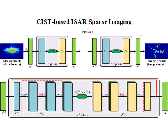
3. Proposed CIST-Based Imaging Method
3.1. Network Model
3.2. Algorithm Flow
3.3. Loss Function
4. Experiments
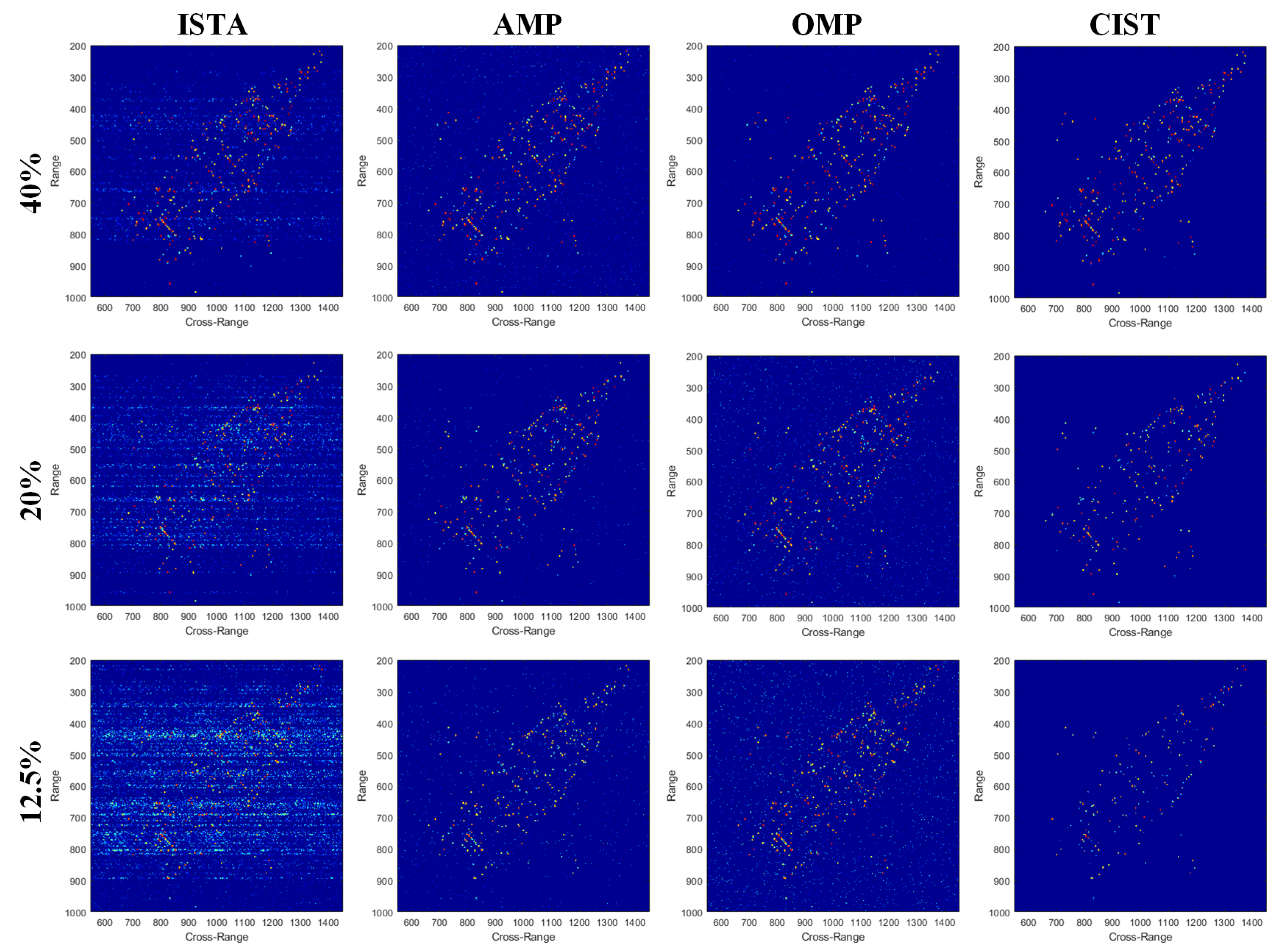
4.1. Simulated Data
4.2. Measured Data
5. Discussion
5.1. Effectiveness of Convolution Layer
5.2. Prospect of Network-Based ISAR Sparse Imaging Methods
6. Conclusions and Future Work
Author Contributions
Funding
Conflicts of Interest
References
- Chen, C.; Andrews, H.C. Target-Motion-Induced Radar Imaging. IEEE Trans. Aerosp. Electron. Syst. 1980, AES-16, 2–14. [Google Scholar] [CrossRef]
- Chen, V.C. Inverse Synthetic Aperture Radar Imaging: Principles, Algorithms and Applications; Institution of Engineering and Technology: Stevenage, UK, 2014. [Google Scholar]
- Chen, V.; Martorella, M. Inverse Synthetic Aperture Radar; Scitech Publishing: Raleigh, NC, USA, 2014. [Google Scholar]
- Xu, G.; Xing, M.; Zhang, L.; Duan, J.; Chen, Q.; Bao, Z. Sparse Apertures ISAR Imaging and Scaling for Maneuvering Targets. IEEE J. Sel. Top. Appl. Earth Obs. Remote Sens. 2014, 7, 2942–2956. [Google Scholar] [CrossRef]
- Candes, E.J.; Tao, T. Decoding by linear programming. IEEE Trans. Inf. Theory 2005, 51, 4203–4215. [Google Scholar] [CrossRef]
- Ender, J.H.G. On Compressive Sensing Applied to Radar. Signal Process. 2010, 90, 1402–1414. [Google Scholar] [CrossRef]
- Wang, L.; Loffeld, O.; Ma, K.; Qian, Y. Sparse ISAR imaging using a greedy Kalman filtering approach. Signal Process. 2017, 138, 1–10. [Google Scholar] [CrossRef]
- Hu, C.; Wang, L.; Li, Z.; Zhu, D. Inverse Synthetic Aperture Radar Imaging Using a Fully Convolutional Neural Network. IEEE Geosci. Remote Sens. Lett. 2019, 17, 1–5. [Google Scholar] [CrossRef]
- Hu, C.; Li, Z.; Wang, L.; Guo, J.; Loffeld, O. Inverse Synthetic Aperture Radar Imaging Using a Deep ADMM Network. In Proceedings of the 20th International Radar Symposium (IRS), Ulm, Germany, 26–28 June 2019; pp. 1–9. [Google Scholar] [CrossRef]
- Zhang, S.; Liu, Y.; Li, X. Fast Sparse Aperture ISAR Autofocusing and imaging via ADMM based Sparse Bayesian Learning. IEEE Trans. Image Process. 2019, 29, 3213–3226. [Google Scholar] [CrossRef]
- Zhang, L.; Xing, M.; Qiu, C.; Li, J.; Bao, Z. Achieving Higher Resolution ISAR Imaging With Limited Pulses via Compressed Sampling. IEEE Geosci. Remote Sens. Lett. 2009, 6, 567–571. [Google Scholar] [CrossRef]
- Liu, H.; Jiu, B.; Liu, H.; Bao, Z. Superresolution ISAR Imaging Based on Sparse Bayesian Learning. IEEE Trans. Geosci. Remote Sens. 2014, 52, 5005–5013. [Google Scholar]
- Zhang, X.; Bai, T.; Meng, H.; Chen, J. Compressive Sensing-Based ISAR Imaging via the Combination of the Sparsity and Nonlocal Total Variation. IEEE Geosci. Remote Sens. Lett. 2014, 11, 990–994. [Google Scholar] [CrossRef]
- Boyd, S.; Parikh, N.; Chu, E.; Peleato, B.; Eckstein, J. Distributed Optimization and Statistical Learning via the Alternating Direction Method of Multipliers; Now Publishers Inc.: Delft, The Netherlands, 2011. [Google Scholar]
- Mousavi, A.; Baraniuk, R.G. Learning to invert: Signal recovery via Deep Convolutional Networks. In Proceedings of the IEEE International Conference on Acoustics, Speech and Signal Processing (ICASSP), New Orleans, LA, USA, 5–9 March 2017; pp. 2272–2276. [Google Scholar]
- Mousavi, A.; Patel, A.B.; Baraniuk, R.G. A deep learning approach to structured signal recovery. In Proceedings of the 53rd Annual Allerton Conference on Communication, Control, and Computing (Allerton), Monticello, IL, USA, 29 September–2 October 2015; pp. 1336–1343. [Google Scholar]
- Wang, M.; Wei, S.; Shi, J.; Wu, Y.; Qu, Q.; Zhou, Y.; Zeng, X.; Tian, B. CSR-Net: A Novel Complex-valued Network for Fast and Precise 3-D Microwave Sparse Reconstruction. IEEE J. Sel. Top. Appl. Earth Obs. Remote Sens. 2020. [Google Scholar] [CrossRef]
- Rolfs, B.; Rajaratnam, B.; Guillot, D.; Wong, I.; Maleki, A. Iterative thresholding algorithm for sparse inverse covariance estimation. In Advances in Neural Information Processing Systems; Neural Information Processing Systems Foundation, Inc.: La Jolla, CA, USA, 2012; pp. 1574–1582. [Google Scholar]
- Donoho, D.L.; Maleki, A.; Montanari, A. Message-passing algorithms for compressed sensing. Proc. Natl. Acad. Sci. USA 2009, 106, 18914–18919. [Google Scholar] [CrossRef] [PubMed]
- Cai, T.T.; Wang, L. Orthogonal Matching Pursuit for Sparse Signal Recovery with Noise; Institute of Electrical and Electronics Engineers: Piscataway, NJ, USA, 2011. [Google Scholar]
- Li, G.; Zhang, H.; Wang, X.; Xia, X. ISAR 2-D Imaging of Uniformly Rotating Targets via Matching Pursuit. IEEE Trans. Aerosp. Electron. Syst. 2012, 48, 1838–1846. [Google Scholar] [CrossRef]
- Zhang, Z.; Rao, B.D. Sparse Signal Recovery With Temporally Correlated Source Vectors Using Sparse Bayesian Learning. IEEE J. Sel. Top. Signal Process. 2011, 5, 912–926. [Google Scholar] [CrossRef]
- Xu, G.; Xing, M.; Xia, X.; Chen, Q.; Zhang, L.; Bao, Z. High-Resolution Inverse Synthetic Aperture Radar Imaging and Scaling With Sparse Aperture. IEEE J. Sel. Top. Appl. Earth Obs. Remote Sens. 2015, 8, 4010–4027. [Google Scholar] [CrossRef]
- Tian, B.; Zhang, X.; Wei, S.; Ming, J.; Shi, J.; Li, L.; Tang, X. A Fast Sparse Recovery Algorithm via Resolution Approximation for LASAR 3D Imaging. IEEE Access 2019, 7, 178710–178725. [Google Scholar] [CrossRef]
- Zhang, J.; Ghanem, B. ISTA-Net: Interpretable optimization-inspired deep network for image compressive sensing. In Proceedings of the IEEE Conference on Computer Vision and Pattern Recognition, Salt Lake City, UT, USA, 18–22 June 2018; pp. 1828–1837. [Google Scholar]
- Berizzi, F.; Martorella, M.; Haywood, B.; Dalle Mese, E.; Bruscoli, S. A survey on ISAR autofocusing techniques. In Proceedings of the International Conference on Image Processing, ICIP ’04, Singapore, 24–27 October 2004; Volume 1, pp. 9–12. [Google Scholar]
- Qiang, W.; Niu, W.; Du, K.; Wang, X.-D.; Yang, Y.-A.; Du, W.-B. ISAR autofocus based on image entropy optimization algorithm. In Proceedings of the IEEE Advanced Information Technology, Electronic and Automation Control Conference (IAEAC), Chongqing, China, 19–20 December 2015; pp. 1128–1131. [Google Scholar]
- Donoho, D.L. Compressed sensing. IEEE Trans. Inf. Theory 2006, 52, 1289–1306. [Google Scholar] [CrossRef]
- Candes, E.J.; Romberg, J.; Tao, T. Robust uncertainty principles: Exact signal reconstruction from highly incomplete frequency information. IEEE Trans. Inf. Theory 2006, 52, 489–509. [Google Scholar] [CrossRef]
- Wright, S.J.; Nowak, R.D.; Figueiredo, M.A.T. Sparse reconstruction by separable approximation. In Proceedings of the IEEE International Conference on Acoustics, Speech and Signal Processing, Las Vegas, NV, USA, 31 March–4 April 2008; pp. 3373–3376. [Google Scholar]
- Zhang, J.; Zhao, D.; Jiang, F.; Gao, W. Structural Group Sparse Representation for Image Compressive Sensing Recovery. In Proceedings of the 2013 Data Compression Conference, Snowbird, UT, USA, 20–22 March 2013; pp. 331–340. [Google Scholar]
- Chambolle, A.; De Vore, R.A.; Lee, N.-Y.; Lucier, B.J. Nonlinear wavelet image processing: Variational problems, compression, and noise removal through wavelet shrinkage. IEEE Trans. Image Process. 1998, 7, 319–335. [Google Scholar] [CrossRef]
- He, K.; Zhang, X.; Ren, S.; Sun, J. Deep residual learning for image recognition. In Proceedings of the IEEE Conference on Computer Vision and Pattern Recognition, Las Vegas, NV, USA, 27–30 June 2016; pp. 770–778. [Google Scholar]
- Trabelsi, C.; Bilaniuk, O.; Zhang, Y.; Serdyuk, D.; Subramanian, S.; Santos, J.F.; Mehri, S.; Rostamzadeh, N.; Bengio, Y.; Pal, C. Deep Complex Networks. Neural and Evolutionary Computing. arXiv 2017, arXiv:1705.09792. [Google Scholar]
- Kingma, D.; Ba, J. Adam: A Method for Stochastic Optimization. arXiv 2014, arXiv:1412.6980. [Google Scholar]
- Mun, S.; Fowler, J.E. Block Compressed Sensing of Images Using Directional Transforms. In Proceedings of the Data Compression Conference, Cairo, Egypt, 7–10 November 2010; p. 547. [Google Scholar]
- Candes, E.J.; Romberg, J.; Tao, T. Stable signal recovery from incomplete and inaccurate measurements. Commun. Pure Appl. Math. 2006, 59, 1207–1223. [Google Scholar] [CrossRef]
- Candes, E.J.; Tao, T. Near-Optimal Signal Recovery From Random Projections: Universal Encoding Strategies? IEEE Trans. Inf. Theory 2006, 52, 5406–5425. [Google Scholar] [CrossRef]
- Gregor, K.; LeCun, Y. Learning Fast Approximations of Sparse Coding. In Proceedings of the 27th International Conference on International Conference on Machine Learning; Omnipress: Madison, WI, USA, 2010; pp. 399–406. [Google Scholar]


| Ratio | Method | NMSE | TCR (dB) | ENT | FA (%) | Time (s) |
|---|---|---|---|---|---|---|
| 40% | ISTA | 0.7426 | 20.3126 | 1.0056 | 7.9273 | 44.5487 |
| AMP | 0.6599 | 45.8388 | 0.3912 | 8.2295 | 71.6221 | |
| OMP | 0.6977 | 39.3184 | 0.4570 | 3.8948 | 468.1091 | |
| CIST | 0.6313 | 50.8584 | 0.3834 | 2.8658 | 0.9031 | |
| 20% | ISTA | 1.5125 | 7.4179 | 1.4951 | 13.8876 | 20.9817 |
| AMP | 1.8814 | −1.8350 | 3.0402 | 37.5987 | 33.1211 | |
| OMP | 0.7171 | 20.5169 | 0.5231 | 4.4982 | 230.7727 | |
| CIST | 0.6730 | 33.5822 | 0.6981 | 2.0802 | 0.8641 | |
| 12.5% | ISTA | 5.6054 | −10.9690 | 3.4825 | 40.2085 | 12.7870 |
| AMP | 0.7158 | 14.4029 | 1.4040 | 10.0269 | 18.2701 | |
| OMP | 0.6977 | 37.3184 | 0.4570 | 3.8948 | 179.2718 | |
| CIST | 0.6596 | 38.7568 | 0.3838 | 1.0618 | 0.8732 |
| Ratio | Method | NMSE | TCR (dB) | ENT | FA (%) | Time (s) |
|---|---|---|---|---|---|---|
| 40% | ISTA | 4.8811 | −5.4672 | 4.7616 | 79.4230 | 31.3632 |
| AMP | 2.9544 | −3.7446 | 3.3459 | 41.8848 | 70.0527 | |
| OMP | 0.6778 | 9.4313 | 0.5125 | 4.4954 | 435.4453 | |
| CIST | 0.6116 | 26.7183 | 0.5187 | 3.8697 | 0.9025 | |
| 20% | ISTA | 5.6621 | −12.2639 | 4.9115 | 75.0532 | 15.7180 |
| AMP | 1.1017 | 1.9251 | 1.7633 | 17.7155 | 34.2185 | |
| OMP | 0.7073 | 2.4763 | 0.8527 | 5.5791 | 229.8903 | |
| CIST | 0.6844 | 23.7948 | 1.0959 | 4.8680 | 0.8723 | |
| 12.5% | ISTA | 7.1987 | −16.9600 | 4.9618 | 65.9731 | 9.7665 |
| AMP | 0.8076 | 23.0803 | 1.6008 | 15.0631 | 18.7310 | |
| OMP | 0.7447 | 20.5169 | 0.5231 | 4.4982 | 183.8871 | |
| CIST | 0.7443 | 24.3366 | 0.5012 | 1.3129 | 0.8852 |
| Ratio | Method | TCR (dB) | ENT | Time (s) |
|---|---|---|---|---|
| 40% | ISTA | 22.2390 | 0.0383 | 28.1188 |
| AMP | 18.0834 | 0.0749 | 41.7755 | |
| OMP | 8.8795 | 0.4223 | 423.0314 | |
| CIST | 22.3466 | 0.0222 | 0.8882 | |
| 20% | ISTA | 23.2729 | 0.0314 | 14.2475 |
| AMP | 23.1530 | 0.0229 | 44.3105 | |
| OMP | 10.4075 | 0.4142 | 206.7307 | |
| CIST | 23.4010 | 0.0206 | 0.8876 | |
| 12.5% | ISTA | 23.3454 | 0.0191 | 9.0207 |
| AMP | 29.5635 | 0.0074 | 27.7906 | |
| OMP | 11.1394 | 0.2510 | 44.4780 | |
| CIST | 22.5672 | 0.2418 | 0.8742 |
| Ratio | Method | TCR (dB) | ENT | Time (s) |
|---|---|---|---|---|
| 40% | ISTA | 11.1156 | 0.3193 | 36.8382 |
| AMP | 12.6834 | 0.5329 | 43.9997 | |
| OMP | 17.6741 | 0.2568 | 122.7069 | |
| CIST | 18.8741 | 0.2015 | 0.8863 | |
| 20% | ISTA | 11.2704 | 0.2417 | 23.4636 |
| AMP | 12.3927 | 0.4850 | 32.6397 | |
| OMP | 17.3148 | 0.2602 | 79.3270 | |
| CIST | 21.3082 | 0.1222 | 0.8754 | |
| 12.5% | ISTA | 11.1156 | 0.3193 | 36.8382 |
| AMP | 11.9356 | 0.3537 | 28.8230 | |
| OMP | 17.6741 | 0.2568 | 122.7069 | |
| CIST | 18.9328 | 0.2473 | 0.8692 |
© 2020 by the authors. Licensee MDPI, Basel, Switzerland. This article is an open access article distributed under the terms and conditions of the Creative Commons Attribution (CC BY) license (http://creativecommons.org/licenses/by/4.0/).
Share and Cite
Wei, S.; Liang, J.; Wang, M.; Zeng, X.; Shi, J.; Zhang, X. CIST: An Improved ISAR Imaging Method Using Convolution Neural Network. Remote Sens. 2020, 12, 2641. https://doi.org/10.3390/rs12162641
Wei S, Liang J, Wang M, Zeng X, Shi J, Zhang X. CIST: An Improved ISAR Imaging Method Using Convolution Neural Network. Remote Sensing. 2020; 12(16):2641. https://doi.org/10.3390/rs12162641
Chicago/Turabian StyleWei, Shunjun, Jiadian Liang, Mou Wang, Xiangfeng Zeng, Jun Shi, and Xiaoling Zhang. 2020. "CIST: An Improved ISAR Imaging Method Using Convolution Neural Network" Remote Sensing 12, no. 16: 2641. https://doi.org/10.3390/rs12162641
APA StyleWei, S., Liang, J., Wang, M., Zeng, X., Shi, J., & Zhang, X. (2020). CIST: An Improved ISAR Imaging Method Using Convolution Neural Network. Remote Sensing, 12(16), 2641. https://doi.org/10.3390/rs12162641