Article

SAR Image Despeckling by Deep Neural Networks: from a Pre-Trained Model to an End-to-End Training Strategy

1
LTCI, Télécom Paris, Institut Polytechnique de Paris, F-91120 Palaiseau, France
2
Electronic Information School, Wuhan University, Wuhan 430072, China
3
Univ Lyon, UJM-Saint-Etienne, CNRS, Institut d Optique Graduate School, Laboratoire Hubert Curien UMR 5516, F-42023 Saint-Etienne, France
*
Author to whom correspondence should be addressed.
Remote Sens. 2020, 12(16), 2636; https://doi.org/10.3390/rs12162636
Submission received: 26 June 2020 / Revised: 4 August 2020 / Accepted: 7 August 2020 / Published: 15 August 2020

Abstract

:
Speckle reduction is a longstanding topic in synthetic aperture radar (SAR) images. Many different schemes have been proposed for the restoration of intensity SAR images. Among the different possible approaches, methods based on convolutional neural networks (CNNs) have recently shown to reach state-of-the-art performance for SAR image restoration. CNN training requires good training data: many pairs of speckle-free/speckle-corrupted images. This is an issue in SAR applications, given the inherent scarcity of speckle-free images. To handle this problem, this paper analyzes different strategies one can adopt, depending on the speckle removal task one wishes to perform and the availability of multitemporal stacks of SAR data. The first strategy applies a CNN model, trained to remove additive white Gaussian noise from natural images, to a recently proposed SAR speckle removal framework: MuLoG (MUlti-channel LOgarithm with Gaussian denoising). No training on SAR images is performed, the network is readily applied to speckle reduction tasks. The second strategy considers a novel approach to construct a reliable dataset of speckle-free SAR images necessary to train a CNN model. Finally, a hybrid approach is also analyzed: the CNN used to remove additive white Gaussian noise is trained on speckle-free SAR images. The proposed methods are compared to other state-of-the-art speckle removal filters, to evaluate the quality of denoising and to discuss the pros and cons of the different strategies. Along with the paper, we make available the weights of the trained network to allow its usage by other researchers.

Graphical Abstract

1. Introduction

Synthetic Aperture Radar (SAR) provides high-resolution, day-and-night and weather-independent images. SAR technology is widely used for remote sensing in Earth observation applications. With advanced techniques, like polarimetry, interferometry and differential interferometry, SAR images have numerous applications, ranging from environmental system monitoring, city sustainable development, disaster detection applications up to planetary exploration [1]. SAR is an active system that makes measurements by illuminating a scene and measuring the coherent sum of several backscattered echoes. As such, the measured signal suffers from strong fluctuations, that appears in the images as a granular “salt and pepper” noise: the speckle phenomenon. The presence of speckle in an image reduces the ability of a human observer to resolve fine details within the image [2] and impacts automatic image analysis tools.
It is well-known that the speckle phenomenon is caused by the presence of many elemental scatterers within a resolution cell, each back-scattering an echo with a different phase shift. The coherent summation of all these echoes produces strong fluctuations of the resulting intensity from one cell to the next [3]. Speckle analysis and reduction is a longstanding topic in SAR imagery. The literature on this topic is extensive and goes from single polarization data to fully polarimetric SAR images (see the reviews [4,5]). Among the different possible strategies, we classify some commonly used despeckling algorithms into the following three categories.
(i) Selection based methods. The simplest way to reduce SAR speckle is to average neighboring pixels within a fixed window. This technique is called spatial multilooking. To reduce the degradation of the spatial resolution when applied to edges, lines or point-link scatterers, both local [6,7,8] and non-local approaches [9,10,11,12] have been proposed.
(ii) Variational methods. These methods formulate the restoration problem as an optimization problem, to find the underlying image which best explains the observed speckle-corrupted image. The objective function to be minimized is typically composed of two terms: a data-fitting term (that uses a Gamma [13], Rayleigh [14] or Fisher–Tippett distribution [15] to model the distribution of SAR images) and a regularization term (the total variation TV has been widely used in the literature [15,16,17,18,19]).
(iii) Transform based methods. Various scientific methods have considered the application of a wavelet transform for despeckling [20,21,22,23], but the estimation of the parameters of the signal and noise statistics is a difficult task. To apply the state-of-the-art methods designed for additive-noise removal in a more straightforward fashion, a logarithmic transformation (a.k.a. a homomorphic transform) is often applied to convert the multiplicative behavior of speckle into an additive component. Xie et al. [24] have derived the statistical distribution of log-transformed speckle noise. Many despeckling methods based on a homomorphic transform have been proposed [25,26,27,28,29]. Special care must be taken because, after a log-transform, the speckle is stationary but not Gaussian and not even centered. At least a debiasing step must be included to account for the expectation of log-transformed speckle, as proposed in [30] and discussed in Section 3.2.2.
Deep learning allows computational models formed of multiple processing layers to learn representations of data that include several levels of abstraction [31]. In recent years, these methods have dramatically improved the state-of-the-art in many computer vision fields, such as object detection [32], face recognition [33], and low-level image processing tasks [34]. Among them, convolutional neural networks (CNNs) with very deep architecture [35], displaying a large capacity and flexibility to represent image characteristics, are well-suited for image restoration. Dong et al. [36] proposed an end-to-end CNN mapping between the low/high-resolution images for single image super-resolution, which demonstrated state-of-the-art restoration quality, and achieved fast speed for practical on-line usage. CNN networks have also been applied to the denoising of natural images, but mostly in the context of additive white Gaussian noise (AWGN). Zhang et al. proposed a feed-forward denoising convolutional neural networks (DnCNN) to embrace the progress in very deep architecture. The advanced regularization and learning methods, including Rectifier Linear Unit (ReLU), batch normalization and residual learning [37] are adopted, dramatically improving the denoising performance. There are also some researches ongoing on non-AWGN denoising tasks, such as salt-and-pepper noise [38], multiplicative noise [39], and blind inpainting [40]. For SAR image despeckling, CNNs have been first used to learn an implicit model in [41]. More and more SAR despeckling methods are now based on deep architectures [42,43,44].
In this paper, we try to shed light on the advantages and disadvantages of making a significant effort to create training sets and learning SAR-specific CNNs rather than readily applying generic networks pre-trained for AWGN removal on natural images to SAR despeckling. We believe that considering this question for intensity images is enlightening for the more difficult case of multi-channel SAR despeckling that arises in SAR polarimetry, SAR interferometry or SAR tomography.
In order to discuss this matter, we consider two different SAR despeckling frameworks based on CNNs. The first one consists of applying a CNN pre-trained on AWGN removal from natural images. Many CNNs have been proposed for AWGN suppression. The extension to SAR imagery requires to account for the statistics of speckle noise. This can be performed by an iterative scheme recently introduced for speckle reduction: MuLoG algorithm [30], which is based on the plug-in ADMM strategy [45]. In the second approach, a network is trained specifically on SAR images. To that end, we describe a new procedure to generate a high-quality training set. We consider a network architecture similar to that used in the work of Chierchia et al. [41] and discuss the influence of the number of layers and of the loss function on the despeckling performance of the CNN, trained and tested on our datasets. The performance of despeckling methods based on deep neural networks depends not only on the network architecture but also on the training set and on the optimization of the network. Published results are then difficult to reprduce, unless the network architecture and weights are released. To facilitate comparisons of future despeckling methods with our work, we provide an open-source code that includes the network weights for Sentinel-1 image despeckling (see Section 5). We have also experimented a hybrid approach, in the sense that the generated SAR dataset has been used to train a CNN for AWGN removal on images whose content is the same as in the task that it will perform.
The remainder of the paper is organized as follows. Section 2 provides a detailed survey of related image denoising works using CNNs. Section 3 first introduces the statistics of SAR data, and then presents the two different SAR despeckling strategies considered in the paper, plus the hybrid approach. In Section 4, extensive experiments are conducted to evaluate restoration performance. Finally, our concluding remarks are given in Section 5 and Section 6.

2. Related Works

The goal of image denoising is to recover a clean image x from a noisy observation y which follows a specific image degradation model. In this paper, we discuss two common degradation models: additive noise ( y = x + n ) and multiplicative noise ( y = x × n ), where n is a random component referred to as “the noise” (the terminology “noise” to describe fluctuations due to speckle is sometimes considered misleading in the context of SAR imaging given that a pair of images acquired under an interferometric configuration have correlated speckle components, which makes it possible to extract meaningful information from the interferometric phase; we will, however, stick to the terminology common in image processing by referring to the speckle as a noise term throughout the paper since we focus on the restoration of intensity-only images).

2.1. Additive Gaussian Noise Eeduction by Deep Learning

In the additive model, one usual assumption is that the noise component n corresponds to an additive white Gaussian noise (AWGN). To perform the estimation of x, a maximum a posteriori (MAP) estimation is often considered, where the goal is to maximize the posterior probability:
x ^ = arg max x p x | y = arg min x log p y | x log p x ,
with p y | x the likelihood defining the noise model, and p x the prior distribution corresponding to the statistical model of clean images. Under an additive white Gaussian noise assumption, the term log p y | x takes the form of a sum of squares: log p y | x = 1 2 σ 2 y x 2 2 , with σ the standard deviation of the noise. The MAP estimator then corresponds to:
x ^ = arg min x 1 2 σ 2 y x 2 2 + g ( x ) = prox σ 2 g ( y ) ,
where g ( x ) = log p x and the notation prox g defines the proximal operator associated to function g [46,47]. Classical prior models g include the total variation, sparse analysis and sparse synthesis priors [48]. While earlier models were handcrafted ( 1 norm of the wavelet coefficients for a specifically chosen transform, total variation), more recent models are learned from sets of natural images (field of experts [49], higher-order Markov random fields [50]).
Beyond MAP estimators, several patch-based methods were designed to estimate the clean image x, such as BM3D [51], LSSC [52] or WNNM [53]. These methods exploit the self-similarity observed in most natural images (repetition of similar structures/textures at the scale of a patch of size typically 8 × 8 within extended neighborhoods).
In order to learn richer patterns of natural images, deep neural networks have been considered for denoising purposes. After the training step, the estimation step is very fast, especially on graphical processing units (GPUs). The first network architectures designed for denoising were trained to learn a mapping from noisy images y to clean ones x by making use of a CNN with feature maps [54], a multi-layer perceptron (MLP) [55], a stacked denoising autoencoder (SDA) network [56], a stacked sparse denoising auto-encoder architecture [40], among all.
More recent networks are trained to estimate the noise component n, i.e., to output the residual y x . This strategy, called “residual learning” [37], has shown to be more efficient when the neural network contains many layers (i.e., for deep networks). In [57], this residual learning formulation for model learning is adopted and 17 layers are used with the 2 loss function. Wang et al. [58] replaced the convolution layer by dilated convolution. In [59,60], an exponential linear unit or soft shrinkage function are used as activation function (i.e., the non-linear step that follows the convolution), instead of the Rectified Linear Unit (ReLU). Liu et al. [61] discuss the relation between the width and the depth of the network. They introduce wide inference networks with only 5 layers. In [62], a wavelet transform is introduced into deep residual learning.
All these variations on a common structure are motivated by finding a trade-off between the network expressivity (in particular, by increasing the size of the receptive field) and the generalization potential (i.e., fighting against the over-fitting phenomenon that arises when the number of network parameters increases).
Most networks generate an estimate x ^ of the clean image from a noisy image y by simple traversal of the feedforward network (and possibly subtracting the residuals to the noisy image, in case of residual learning): the proximal operator prox g is learned instead of the prior distribution p ( x ) , no explicit minimization is performed when estimating a denoised image. The plug-and-play ADMM strategy [45] provides a means to apply implicit modeling of the prior distribution p ( x ) encoded within the network in the form of the proximal operator prox g in order to address more general image restoration problems than the mere AWGN removal.

2.2. Speckle Reduction by Deep Learning

In the past years, most of the SAR image denoising approaches are based on detailed statistical models of signal and speckle. To avoid the problem of modeling the statistical distribution of speckle-free SAR images, several authors recently resorted to machine learning approaches implemented through CNNs.
The first paper that investigates the problem of SAR image despeckling through CNNs is [41]. Following the paradigm proposed in [57], the SAR-CNN implemented by Chierchia et al. is trained in a residual fashion, where a homomorphic approach [30] is used in order to stabilize the variance of speckle noise. The network comprises 17 convolutional layers with Batch Normalization [63] and Rectifier Linear Units (ReLU) [35] activation function. Logarithm and hyperbolic cosine are combined in a smoothed 1 loss function. The Image Despeckling Convolutional Neural Network (ID-CNN) proposed by Wang et al. [64] comprises only 8 layers and is applied directly on the input image without a log-transform. The novelty lies in the formulation of the loss function as a combination of an 2 loss and of Total Variation (TV), preventing the apparition of artifacts while preserving important details such as edges. In [43], the proposed SAR-DRN makes use of dilated convolutions and skip connections to increase the receptive field without increasing the complexity of the network and maintaining the advantages of 3 × 3 filters. Wang et al. [42] tackle the image despeckling problem by resorting to generative adversarial networks. In the proposed ID-GAN, the Generator is trained to directly estimate the clean image from a noisy observation, while the discriminator serves to distinguish the de-speckled image synthesized by the generator from the corresponding ground truth image. To exploit the abundance of stacks of multitemporal data and avoid the problem of creating a clean reference, in [44] a CNN is used as an auto-encoder through a formulation that does not use an explicit expression of the noise model, thus allowing generalization.

3. SAR Despeckling Using CNNs

3.1. Statistics of SAR Images

After SAR focusing, the SAR image is formed by the collection of the complex amplitudes back-scattered by each resolution cell. The squared modulus of this complex amplitude (the intensity image) is informative of the total reflectivity of the scatterers in each resolution cell. Because of the interference between echoes produced by elementary scatterers, the intensity fluctuates (speckle phenomenon). These fluctuations depend on the 3-D spatial configuration of the scatterers with respect to the SAR system and on the nature of the scatterers. They are generally modeled by Goodman’s stochastic model (fully developed speckle): the measured intensity y is related to the reflectivity x by the multiplicative model y = x × n where the noise component n R + is a random variable that follows a gamma distribution [3]:
p ( n ) = L L Γ ( L ) n L 1 exp L n ,
with L 1 representing the number of looks, and Γ ( · ) the gamma function. It follows from E [ n ] = 1 and Var [ n ] = 1 / L that E [ y ] = x : averaging the intensity leads to an unbiased estimator of the reflectivity in stationary areas, and Var [ y ] = x 2 / L : the noise is signal-dependent in the sense that the variance of the measured intensity increases like the square of the reflectivity.
Considering the log of the intensity y ˜ instead of the intensity y transforms the noise into an additive component: y ˜ = x ˜ + n ˜ where n ˜ R follows a Fisher-Tippett distribution [24]:
p ( n ˜ ) = L L Γ ( L ) e L n ˜ exp ( L e n ˜ ) .
The mean E [ n ˜ ] = ψ ( L ) log ( L ) ( ψ is digamma function) is non-zero, which indicates that averaging log-transformed intensities y ˜ leads to a biased estimate of the log-reflectivity x ˜ . The variance Var [ n ˜ ] = ψ ( 1 , L ) (where ψ ( 1 , L ) is the polygamma function of order L [65]) does not depend on the reflectivity: it is stationary over the image.

3.2. Despeckling Using Pre-Trained CNN Models

As discussed in Section 2, several approaches have been recently proposed in the literature to apply CNNs to AWGN suppression. The residual learning method DnCNN introduced in [57] is a reference method for which models pre-trained on natural images at various signal-to-noise ratios are available (https://github.com/cszn/DnCNN). We consider two different ways to apply a pre-trained CNN to speckle noise reduction: a homomorphic filter that processes log-transformed intensities with DnCNN and the embedding of DnCNN within the iterative scheme MuLoG [30]. Note that our approach is general and other pre-trained CNNs than the DnCNN could readily be applied.

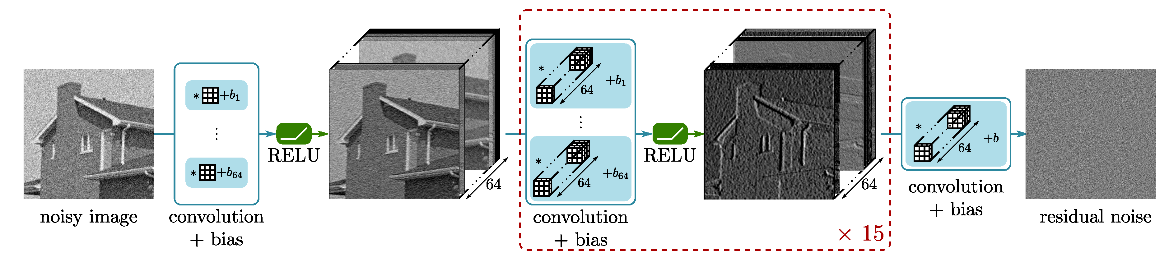
3.2.1. Architecture of the CNN

Figure 1 and Table 1 illustrate the architecture of the network DnCNN proposed by Zhang et al. [57]. The network is a modified VGG network and is made of 17 fully convolutional layers with no pooling. There are three types of layers: (i) Conv+ReLU: for the first layer, 64 filters of size 3 × 3 are used to generate 64 feature maps, and rectified linear units are then utilized for nonlinearity; (ii) Conv+BN+ReLU: for layers 2∼16, 64 filters of size 3 × 3 × 64 are used, and batch normalization is added between convolution and ReLU; (iii) Conv: for the last layer, a filter of size 3 × 3 × 64 is used to reconstruct the output. The loss function that is minimized during the training step is the 2 loss (i.e., the sum of squared errors, averaged over the whole training set). To train the DnCNN, 400 natural images of size 180×180 pixels with gray levels in the range [ 0 , 1 ] were used for training. Patches of size 40 × 40 pixels were extracted at random locations from these images. Different networks were trained for simulated additive white Gaussian noise levels equal to σ = 10 255 , 15 255 , . . . , 75 255 (14 different networks each corresponding to a given noise standard deviation).

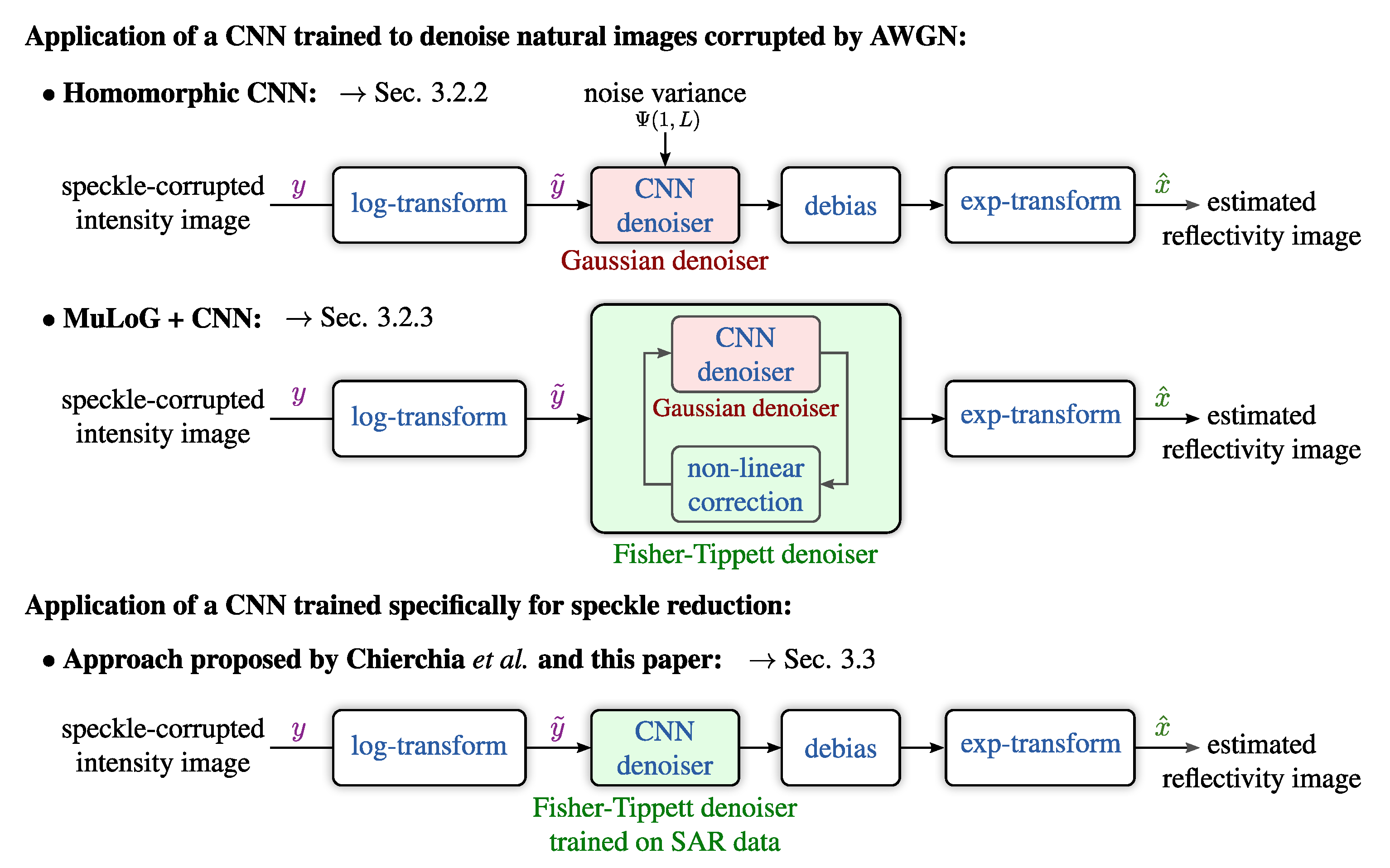
3.2.2. Homomorphic Filtering with a Pre-Trained CNN

The simplest approach to applying a pre-trained CNN acting as a Gaussian denoiser is the homomorphic filtering depicted at the top of Figure 2, and hereafter denoted homom.-CNN. This approach consists of approximating the noise term n ˜ in log-transformed data as an additive white Gaussian noise with non-zero mean. As recalled in Section 3.1, log-transformed speckle is not Gaussian but follows a Fisher-Tippett distribution under Goodman’s fully developed speckle model. Hence, the homomorphic approach is built on a rather coarse statistical approximation. Under this approximation, the log-transformed SAR image can be restored by first applying the pre-trained CNN, then correcting for the bias ψ ( L ) log L due to the non-centered noise component.
In order to successfully apply a pre-trained CNN model, it is crucial to properly normalize the data so that the range of input data matches the range of data used during the training step (neural networks are highly non-linear). This paper maps the range [ q m , q M ] by an affine transform to the [ 0 , 1 ] range, with q m and q M corresponding to the 0.3 % and 99.7 % quantiles of the log-transformed intensities. After this normalization, the standard deviation of the log-transformed noise is σ = ψ ( 1 , L ) / ( q M q m ) . This value can be used to select the network trained for the closest noise standard deviation σ train that is less or equal to σ . The normalized image is then multiplied by σ train / σ so that the noise standard deviation exactly matches that of the images in the training set of the network.

3.2.3. Iterative Filtering with MuLoG and a Pre-Trained Model

The MuLoG framework [30] accounts for the Fisher-Tippett distribution of log-transformed speckle (see Figure 3) with an iterative scheme that alternates the application of a Gaussian denoiser (namely, a proximal operator) and of a non-linear correction. Figure 2, second row, illustrates that, by embedding a CNN trained as a Gaussian denoiser within an iterative scheme, a Fisher-Tippett denoiser is obtained. Throughout the iterations, the parameter of the Gaussian denoiser evolves, which requires to apply the network selection and image normalization strategy described in the previous paragraph.

3.3. Despeckling with a CNN Specifically Trained on SAR Images

The architecture that we consider for our CNN trained on SAR images (SAR-CNN) is based on the work of Chierchia et al. [41], who in turn was inspired by the DnCNN by Zhang et al. [57] that we described in Section 3.2.1. In this section, we describe in details a procedure for producing high-quality ground-truth images for the training step of the network.

3.3.1. Training-Set Generation

Deep learning models need a lot of data to generalize well. This is an issue in deep learning-based SAR image despeckling techniques, due to the lack of truly speckle-free SAR images. The reference image has to be therefore created through an ad-hoc procedure, in order to produce images taking into account the content of SAR data (strong backscattering scatterers, real radiometric contrasts of SAR data). This is done by exploiting series of SAR images.
Speckle noise can be strongly reduced by multi-temporal multilooking (i.e., averaging the intensity of images acquired at different dates, assuming that no changes occurred). Multi temporal stacks have therefore been considered in this study. Due to the coherence of some regions, some speckle fluctuations are remaining after this temporal multi-looking procedure. These images are further improved by applying a MuLoG+BM3D denoising step [30] with an equivalent number of looks estimated from selected homogeneous regions. The images obtained are then considered speckle-free and serve as a ground truth. Synthetic speckle noise is simulated based on the statistical models described in Section 3.1 in order to produce the noisy/clean image pairs necessary for the training of the network. Although Goodman’s fully developed model is not verified everywhere in the images (the Rician distribution [66,67,68] could instead be used for strong scatterers) and assumes spatially uncorrelated speckle, it has been the funding model of most SAR despeckling methods developed these last four decades [16]. Thus, we find it relevant to simulate 1-look speckle noise based on Goodman’s model. In Section 4.3, its limitations are discussed.
A ground truth image is depicted in Figure 4, where we show the progress from the 1-look SAR image to the clean reference used in our training step. The temporal average of large temporal stacks of finely registered SAR images leads to images with limited speckle fluctuations and, after denoising, these images retain the characteristics of SAR images (bright points, sharp edges, textures) with almost no residual fluctuations due to speckle. Since the denoising operation is applied on an image already temporally multilooked, only small fluctuations have to be suppressed by the denoising step (i.e., this denoising step helps but is not crucial). This method thus proposes a realistic way to create speckle-free SAR images. A description of the training set is then given in Table 2.

3.3.2. Network Architecture and the Effect of the Loss Function

The network is easier to train on log-transformed data since the noise is then additive and white (and coarsely Gaussian distributed, as it ca be seen from Figure 3). Compared to the suppression of AWGN, the networks need to learn how to separate log-transformed SAR reflectivities from log-transformed speckle, distributed according to the Fisher-Tippett distribution given in Equation (4). In the follwing, a discussion about minor changes to the network architecture is carried out. It is worth to point out that, given the impossibility to reproduce the work proposed in [41] (the weights are not available and the datasets are not the same), we intend by no means to compare our results to those of Chierchia et al. Instead, we have always followed our training strategy and drawn conclusions based on visual inspection of our testing set.
In this study, it has been experimentally found that increasing the depth of the network compared to the depth used by Zhang et al. and Chierchia et al. was improving the performance on the testing set. We used 19 layers, each layer involving spatial convolutions with 3 × 3 kernels (see Figure 5). The receptive field of our network then corresponds to a patch of size 39 × 39 .
To train the network, several loss functions have been considered. Experiments suggest the 1 loss function to be preferable to the smoothed 1 loss function of Chierchia et al. and to 2 loss function. This matches other studies that have shown a reduction of artifacts and an improvement of the convergence when using the 1 loss [69]. We, therefore, used the following loss function:
i = 1 N f CNN ( y ˜ i ) x ˜ i + ( ψ ( L ) log ( L ) ) · 1 1
where the sum is carried over all N images from (a batch sampled from) the training set, f CNN ( · ) represents the action of the CNN on some log-transformed input data, the boldface is used to denote images (the i-th noisy image y i and the corresponding speckle-free reference x i ). The term ( ψ ( L ) log ( L ) ) · 1 is a constant image that corresponds to the bias correction. Its role is to center Fisher-Tippett distribution. By making this term explicit, it is easier to perform transfer learning, i.e., to re-train a network to a different number of looks L by warm-starting the optimization from the values obtained for the previous number of looks.

3.3.3. The Training of the Network

The training set is formed by 7 Sentinel-1 speckle-free images produced by filtering 7 different multi-temporal stacks of size between 1024 × 1536 and 1024 × 8192 pixels, as described in Section 3.3.1. The images are selected so that to cover urban areas, forests, a coast with some water surfaces, fields and mountainous areas. Patches of size 40 × 40 are extracted from these images, with a stride of 10 pixels between patches. Mini-batches of 128 patches are used. In order to improve the network generalization capability, standard data augmentation techniques are used: vertical, horizontal flipping and ± 90 and 180 rotations are applied on the patches. 11968 batches of 128 patches are processed during an epoch. A total of 50 epochs were used with ADAM stochastic gradient optimization method, with an initial learning rate of 0.001. The convergence of the learning and prevention for over-fitting were checked by monitoring the decrease of the loss function throughout the epochs as well as the performance over the test set. The deep learning framework used for the implementation is tensorflow 1.1.12. Training is carried out with an Intel Xeon CPUat 3.40 GHz and an Nvidia K80 GPU and took approximately 7 h.

3.4. Hybrid Approach: MuLoG + Trained CNN

A hybrid approach is also considered. In this method, the dataset that we have constructed is used to retrain the CNN described in Section 3.2.1 to remove Gaussian noise from SAR images. Account for the Fisher-Tippett distribution is also made possible by embedding this network within the MuLoG framework. By doing so, we aim at investigating the influence of the content of the training images on the restoration performances.

4. Experimental Results

The following paragraphs provide a comparison of the different strategies for CNN-based despeckling both on images with simulated speckle and on single-look Sentinel-1 images. First, the impact of the loss function and of the number of layers on the performance of SAR-CNN is illustrated. Network architecture is described in Section 3.2.1 and Section 3.3.2 (and more in details in the original article [57]). A graphic illustration is also provided in Figure 5. The network has been trained in a supervised way using a dataset created as explained in Section 3.3.1. The three proposed algorithms are summarized in Table 3.

4.1. Influence of the Loss Function and of the Network Depth

Figure 6 shows the impact of the loss function ( 1 versus the smoothed 1 used by Chierchia et al. [41]) and of the network depth in terms of despeckling artifacts on an image with simulated speckle. The image corresponds to one of the speckle-free images of our testing set. We magnify 6 regions in order to illustrate cases where the initial CNN architecture fails to recover some structures (regions 1, 2, 3 and 6) that are present in the ground truth and at least partially recovered applying the proposed modifications to the CNN, and cases were some spurious structures appear (regions 4 and 5) with the first CNN architecture employed, but are not created with the modifications of the CNN depth and loss function that we considered.
All the three architectures are trained for 50 epochs on the high-quality database of SAR images we have created, and conclusions are drawn after qualitative evaluation of our testing images. Indeed, as already claimed, a comparison with the work of Chierchia et al. is not applicatble.

4.2. Quantitative Comparisons on Images with Simulated Speckle

Two common image quality criteria are used to evaluate the quality of despeckling obtained with different methods: the Peak-signal-to-noise ratio (PSNR), related to the mean squared error, which is relevant in terms of evaluation of the estimated reflectivities (bias and variance of the estimator), and the structural similarity (SSIM) which better captures the perceived image quality. For each speckle-free image from the testing set, several versions corrupted by synthetic single-look speckle are generated, in order to report both the PSNR and SSIM mean values, and their standard deviations over different noise realizations.
Seven different images are used in our testing set. We report the performance of the approaches proposed in this paper as well as the performance of SAR-BM3D [25], NL-SAR [12] and MuLoG+BM3D in Table 4 and Table 5.
To qualitatively evaluate the quality of denoising, we display in Figure 7 the results obtained by the different methods on image “Marais 1”. To better analyze the results, the residual intensity images (i.e., the ratio between the noisy and the restored images) are displayed below the restored images. Almost no structure can be identified by visual analysis of the residual images, which means that the compared methods preserve very well the geometrical content of the original images (limited over-smoothing).
It can be observed both on the quantitative results reported in the tables and in the qualitative analysis that the CNN methods (the two versions of MuLoG+CNN and SAR-CNN) perform better than MuLoG+BM3D which we use as reference algorithm in SAR despeckling before the introduction of CNN methods. SAR-CNN removes speckle from the images while preserving the details, such as edges, at the cost of introducing small but noticeable artifacts in homogeneous areas. Instead, MuLoG+BM3D and MuLoG+CNN generate blurry edges, over-smoothing some areas where the details are lost, even when the CNN is pre-trained on SAR images. This can be observed comparing the denoised images of Figure 7, where SAR-CNN preserves better the details of the urban area at the bottom of the image compared to the three other denoising methods. The quality of the details can be attributed to the richness of information captured by the network when learning on many SAR image patches.

4.3. Despeckling of Real Single-Look SAR Images: How to Handle Correlations

In this section, the denoising performance of SAR-CNN for Sentinel-1 image despeckling and MuLoG+CNN are evaluated on real single-look SAR images acquired during Sentinel-1 mission. To test our deep learning-based denoiser, we focused on some of the areas of the images analyzed in the above tables, picking one of the multitemporal instances used to generate the ground truth images for the training of SAR-CNN and making sure that these areas do not belong to the training set.
Unlike synthetically generated noisy SAR images, in real acquisitions, pixels are spatially correlated. SAR images undergo an apodization (and over-sampling) process [70,71,72] aimed at reducing the sidelobes of strong targets, by introducing some spectral weighting. Thus, we subsample real SAR acquisitions by a factor of 2, as proposed in [73]. As already observed in the case of synthetic SAR data, the images that are restored with the proposed methods show significant improvements on the denoising performance over the reference despeckling algorithm MuLoG+BM3D, with SAR-CNN being the one that provides the best visual result. Even when compared to SAR-BM3D and NL-SAR, which do not require the image to undergo a downsampling step, our results are more good-looking, with a better preservation of fine structures. NL-SAR, indeed, gives its best in polarimetric and interferometric configurations.
Figure 8 shows the restoration results and the residual images (obtained by forming the ratio noisy/denoised) obtained with the different methods. In contrast to the simulated case, some structures can be visually identified in the residual images. These structures correspond to thin roads. The downsampling operation necessary to remove the speckle correlations make the preservation of these structures very difficult for all methods. SAR-CNN seems to be the most effective at preserving those structures. Indeed, the residual image does not present clear textures nor constant areas, meaning that no structures have been removed and that noise there is no noise left in the restored image (the residual image represents what is suppressed from the noisy image). Visual analysis of the restored images compared to the real image also seems to indicate fewer artifacts with SAR-CNN.
Since the ground-truth reflectivity is not available, to measure the performance of the proposed method the Equivalent Number of Looks is estimated on manually selected homogeneous areas. The homogeneous regions chosen for the ENL estimation are shown with red boxes, and the ENL values are given in Table 6.
Then, this analysis has been extended to a TerraSAR-X acquisition. In this case, the study aims at assessing the generalization capabilities of the trained SAR-CNN on images from a different sensor and a different spatial resolution. While MuLoG+CNN is not dedicated to a specific sensor (see Table 7), SAR-CNN is sensor specific. As such, to give its best on TerraSAR-X images, it should be retrained using images acquired from TerraSAR-X: a dataset can be constructed as described in Section 3.3.1. As it can be seen from Figure 9, MuLoG+CNN seems the approach that provides visually the best results. The estimated ENL indicate that all despeckling methods are very effective in homogeneous regions. It seems that MuLoG+CNN produces an image with a slightly better perceived resolution, which may indicate a better generalization property compared to SAR-CNN. While the latter would benefit from a dedicated training on TerraSAR-X images, it achieves satisfying performance on this data without any fine-tuning, which indicates that it could be readily applied to images from other sensors in the absence of time series to build a ground truth for retraining. The analysis of the residual images, like in Figure 8, indicates that thin linear structures are attenuated in restored images due to the downsampling step.

5. Discussion

A CNN trained to suppress additive white Gaussian noise encodes a very generic model of natural images in the form of a proximal operator related to an implicit prior. Like other models of natural images that were successfully applied to the problem of speckle reduction in SAR imaging (wavelets, total variation), they are relevant to SAR imagery because they capture structures (points, edges, corners) and textures. Yet, the specificities of SAR images make it beneficial to train a model specifically on SAR images. This is done naturally by patch-based methods that use the content of the image itself as a model (repeating patches). In this paper, we have shown a considerable improvement with a CNN model trained on SAR images provided that a high-quality training set is built, enough layers are used to capture large scale structures and an adequate loss function is selected. Moreover, once trained, SAR-CNN exhibits the best runtime performance when using a GPU (see Table 7). When considering the real-life case of partially correlated speckle or images from different sensors, the plugging of a network trained on natural images in a SAR adapted framework like MuLoG presents better generalization properties.
The extension to multi-channel SAR images represents a real challenge. Speckle reduction in multi-channel images requires modeling the correlations between channels (the interferometric and polarimetric information). In order to learn those correlations directly from the data, a dataset that contains speckle-free images covering the whole diversity of polarimetric responses, interferometric phase differences and the whole range of coherences for typical geometrical structures (points, lines, corners, homogeneous regions, textured regions) must be formed. Needless to say, this is far more challenging than collecting single-channel SAR images to cover only the diversity of geometric structures. Failure to correctly include all cases in the training set implies that the network, instead of performing a high-dimensional interpolation, performs a high-dimensional extrapolation, which puts the user at high risk of experiencing large prediction errors.
This difficulty justifies the relevance of using pre-trained networks within MuLoG framework which has been designed to apply single-channel restoration methods to multi-channel SAR images. A summary of the advantages and drawbacks of the proposed methods are reported in Table 8. Only a little gain in performance is observed when, considering MuLoG+CNN, the network is pre-trained on SAR images. Thus, if creating a dataset is possible it is advisable to use it to train an end-to-end model such as SAR-CNN.
To offer the possibility to use the presented SAR-CNN for testing and comparison, we release an open-source code of the network trained on our dataset: https://gitlab.telecom-paris.fr/RING/SAR-CNN. Indeed, replicating results of a published work is not an easy task and may represents up to months of work. Therefore, by sharing our code, we hope to help other researchers and users of SAR images to easily apply our CNN-based denoiser on single-look Sentinel-1 images, and possibly compare the restoration performance with their own methods.

6. Conclusions

With the new generation of sensors orbiting around Earth, access to long time-series of SAR images is improving. Given the increasing interest towards the use of deep learning algorithms in SAR despeckling, in this paper it is described a procedure to generate ground truth images that can be applied in a systematic way to produce large training sets formed by pairs of high-quality speckle-free images and simulated speckled images.
In a future work, it would be interesting to train the networks on actual single-look SAR images in order to account for spatial correlations of the speckle. This, however, would require a method to produce a high quality ground-truth image for each single-look observation. Restoration methods that exploit long time-series of SAR images [74] may pave the way to producing such training sets.

Author Contributions

Conceptualization: F.T and L.D.; methodology and formal analysis: E.D., X.Y., L.D., F.T; writing: E.D., X.Y., L.D., F.T.; review and editing: E.D., L.D., F.T.; supervision: L.D., F.T., W.Y., software: L.D., E.D. All authors have read and agreed to the published version of the manuscript.

Funding

This research received no external funding.

Conflicts of Interest

The authors declare no conflict of interest.

References

  1. Moreira, A.; Prats-Iraola, P.; Younis, M.; Krieger, G.; Hajnsek, I.; Papathanassiou, K.P. A tutorial on synthetic aperture radar. IEEE Trans. Geosci. Remote Sens. 2013, 1, 6–43. [Google Scholar] [CrossRef] [Green Version]
  2. Lee, J.S.; Jurkevich, L.; Dewaele, P.; Wambacq, P.; Oosterlinck, A. Speckle filtering of synthetic aperture radar images: A review. Remote Sens. Rev. 1994, 8, 313–340. [Google Scholar] [CrossRef]
  3. Goodman, J.W. Some fundamental properties of speckle. JOSA 1976, 66, 1145–1150. [Google Scholar] [CrossRef]
  4. Touzi, R. A review of speckle filtering in the context of estimation theory. IEEE Trans. Geosci. Remote Sens. 2002, 40, 2392–2404. [Google Scholar] [CrossRef]
  5. Argenti, F.; Lapini, A.; Bianchi, T.; Alparone, L. A tutorial on speckle reduction in Synthetic Aperture Radar images. IEEE Geosci. Remote Sens. Mag. 2013, 1, 6–35. [Google Scholar] [CrossRef] [Green Version]
  6. Lee, J.S.; Grunes, M.R.; De Grandi, G. Polarimetric SAR speckle filtering and its implication for classification. IEEE Trans. Geosci. Remote Sens. 1999, 37, 2363–2373. [Google Scholar]
  7. Lopes, A.; Nezry, E.; Touzi, R.; Laur, H. Structure detection and statistical adaptive speckle filtering in SAR images. Int. J. Remote Sens. 1993, 14, 1735–1758. [Google Scholar] [CrossRef]
  8. Feng, H.; Hou, B.; Gong, M. SAR image despeckling based on local homogeneous-region segmentation by using pixel-relativity measurement. IEEE Trans. Geosci. Remote Sens. 2011, 49, 2724–2737. [Google Scholar] [CrossRef]
  9. Deledalle, C.A.; Denis, L.; Tupin, F. Iterative weighted maximum likelihood denoising with probabilistic patch-based weights. IEEE Trans. Image Process. 2009, 18, 2661–2672. [Google Scholar] [CrossRef] [PubMed] [Green Version]
  10. Deledalle, C.A.; Denis, L.; Tupin, F. NL-InSAR: Nonlocal interferogram estimation. IEEE Trans. Geosci. Remote Sens. 2011, 49, 1441–1452. [Google Scholar] [CrossRef]
  11. Chen, J.; Chen, Y.; An, W.; Cui, Y.; Yang, J. Nonlocal filtering for polarimetric SAR data: A pretest approach. IEEE Trans. Geosci. Remote Sens. 2011, 49, 1744–1754. [Google Scholar] [CrossRef]
  12. Deledalle, C.A.; Denis, L.; Tupin, F.; Reigber, A.; Jäger, M. NL-SAR: A unified nonlocal framework for resolution-preserving (Pol)(In) SAR denoising. IEEE Trans. Geosci. Remote Sens. 2015, 53, 2021–2038. [Google Scholar] [CrossRef] [Green Version]
  13. Baraldi, A.; Parmiggiani, F. A refined Gamma MAP SAR speckle filter with improved geometrical adaptivity. IEEE Trans. Geosci. Remote Sens. 1995, 33, 1245–1257. [Google Scholar] [CrossRef]
  14. Kuruoglu, E.E.; Zerubia, J. Modeling SAR images with a generalization of the Rayleigh distribution. IEEE Trans. Image Process. 2004, 13, 527–533. [Google Scholar] [CrossRef]
  15. Bioucas-Dias, J.M.; Figueiredo, M.A. Multiplicative noise removal using variable splitting and constrained optimization. IEEE Trans. Image Process. 2010, 19, 1720–1730. [Google Scholar] [CrossRef] [Green Version]
  16. Aubert, G.; Aujol, J.F. A variational approach to removing multiplicative noise. Siam J. Appl. Math. 2008, 68, 925–946. [Google Scholar] [CrossRef]
  17. Darbon, J.; Sigelle, M.; Tupin, F. The use of levelable regularization functions for MRF restoration of SAR images while preserving reflectivity. In Computational Imaging V; International Society for Optics and Photonics: Bellingham, WA, USA, 2007; Volume 6498, p. 64980T. [Google Scholar]
  18. Shi, J.; Osher, S. A nonlinear inverse scale space method for a convex multiplicative noise model. Siam J. Imaging Sci. 2008, 1, 294–321. [Google Scholar] [CrossRef] [Green Version]
  19. Denis, L.; Tupin, F.; Darbon, J.; Sigelle, M. SAR image regularization with fast approximate discrete minimization. IEEE Trans. Image Process. 2009, 18, 1588–1600. [Google Scholar] [CrossRef] [Green Version]
  20. Argenti, F.; Alparone, L. Speckle removal from SAR images in the undecimated wavelet domain. IEEE Trans. Geosci. Remote Sens. 2002, 40, 2363–2374. [Google Scholar] [CrossRef]
  21. Dai, M.; Peng, C.; Chan, A.K.; Loguinov, D. Bayesian wavelet shrinkage with edge detection for SAR image despeckling. IEEE Trans. Geosci. Remote Sens. 2004, 42, 1642–1648. [Google Scholar]
  22. Bianchi, T.; Argenti, F.; Alparone, L. Segmentation-based MAP despeckling of SAR images in the undecimated wavelet domain. IEEE Trans. Geosci. Remote Sens. 2008, 46, 2728–2742. [Google Scholar] [CrossRef]
  23. Li, H.C.; Hong, W.; Wu, Y.R.; Fan, P.Z. Bayesian wavelet shrinkage with heterogeneity-adaptive threshold for SAR image despeckling based on generalized Gamma distribution. IEEE Trans. Geosci. Remote Sens. 2013, 51, 2388–2402. [Google Scholar] [CrossRef]
  24. Xie, H.; Pierce, L.E.; Ulaby, F.T. Statistical properties of logarithmically transformed speckle. IEEE Trans. Geosci. Remote Sens. 2002, 40, 721–727. [Google Scholar] [CrossRef]
  25. Parrilli, S.; Poderico, M.; Angelino, C.V.; Verdoliva, L. A nonlocal SAR image denoising algorithm based on LLMMSE wavelet shrinkage. IEEE Trans. Geosci. Remote Sens. 2012, 50, 606–616. [Google Scholar] [CrossRef]
  26. Achim, A.; Tsakalides, P.; Bezerianos, A. SAR image denoising via Bayesian wavelet shrinkage based on heavy-tailed modeling. IEEE Trans. Geosci. Remote Sens. 2003, 41, 1773–1784. [Google Scholar] [CrossRef]
  27. Solbo, S.; Eltoft, T. Homomorphic wavelet-based statistical despeckling of SAR images. IEEE Trans. Geosci. Remote Sens. 2004, 42, 711–721. [Google Scholar] [CrossRef]
  28. Xie, H.; Pierce, L.E.; Ulaby, F.T. SAR speckle reduction using wavelet denoising and Markov random field modeling. IEEE Trans. Geosci. Remote Sens. 2002, 40, 2196–2212. [Google Scholar] [CrossRef] [Green Version]
  29. Bhuiyan, M.I.H.; Ahmad, M.O.; Swamy, M. Spatially adaptive wavelet-based method using the Cauchy prior for denoising the SAR images. IEEE Trans. Circuits Syst. Video Technol. 2007, 17, 500–507. [Google Scholar] [CrossRef]
  30. Deledalle, C.A.; Denis, L.; Tabti, S.; Tupin, F. MuLoG, or how to apply Gaussian denoisers to multi-channel SAR speckle reduction? IEEE Trans. Image Process. 2017, 26, 4389–4403. [Google Scholar] [CrossRef] [PubMed] [Green Version]
  31. LeCun, Y.; Bengio, Y.; Hinton, G. Deep learning. Nature 2015, 521, 436. [Google Scholar] [CrossRef]
  32. Ren, S.; He, K.; Girshick, R.; Sun, J. Faster R-CNN: Towards real-time object detection with region proposal networks. In Advances in Neural Information Processing Systems; NIPS: Montreal, QC, Canada, 2015; pp. 91–99. [Google Scholar]
  33. Sun, Y.; Chen, Y.; Wang, X.; Tang, X. Deep learning face representation by joint identification-verification. In Advances in Neural Information Processing Systems; NIPS: Montreal, QC, Canada, 2014; pp. 1988–1996. [Google Scholar]
  34. Chan, T.H.; Jia, K.; Gao, S.; Lu, J.; Zeng, Z.; Ma, Y. PCANet: A simple deep learning baseline for image classification? IEEE Trans. Image Process. 2015, 24, 5017–5032. [Google Scholar] [CrossRef] [PubMed] [Green Version]
  35. Krizhevsky, A.; Sutskever, I.; Hinton, G.E. Imagenet classification with deep convolutional neural networks. In Advances in Neural Information Processing Systems; NIPS: Lake Tahoe, NV, USA, 2012; pp. 1097–1105. [Google Scholar]
  36. Dong, C.; Loy, C.C.; He, K.; Tang, X. Image super-resolution using deep convolutional networks. IEEE Trans. Pattern Anal. Mach. Intell. 2016, 38, 295–307. [Google Scholar] [CrossRef] [PubMed] [Green Version]
  37. He, K.; Zhang, X.; Ren, S.; Sun, J. Deep residual learning for image recognition. In Proceedings of the IEEE Conference on Computer Vision and Pattern Recognition, Las Vegas, NV, USA, 27–30 June 2016; pp. 770–778. [Google Scholar]
  38. Dong, B.; Ji, H.; Li, J.; Shen, Z.; Xu, Y. Wavelet frame based blind image inpainting. Appl. Comput. Harmon. Anal. 2012, 32, 268–279. [Google Scholar] [CrossRef] [Green Version]
  39. Wang, G.; Pan, Z.; Zhang, Z. Deep CNN Denoiser prior for multiplicative noise removal. Multimed. Tools Appl. 2019, 78, 29007–29019. [Google Scholar] [CrossRef]
  40. Xie, J.; Xu, L.; Chen, E. Image denoising and inpainting with deep neural networks. In Advances in Neural Information Processing Systems; NIPS: Lake Tahoe, NV, USA, 2012; pp. 341–349. [Google Scholar]
  41. Chierchia, G.; Cozzolino, D.; Poggi, G.; Verdoliva, L. SAR image despeckling through convolutional neural networks. In Proceedings of the Geoscience and Remote Sensing Symposium (IGARSS), Fort Worth, TX, USA, 23–28 July 2017; pp. 5438–5441. [Google Scholar]
  42. Wang, P.; Zhang, H.; Patel, V.M. Generative adversarial network-based restoration of speckled SAR images. In Proceedings of the 2017 IEEE 7th International Workshop on Computational Advances in Multi-Sensor Adaptive Processing (CAMSAP), Curacao, The Netherlands, 10–13 December 2017; pp. 1–5. [Google Scholar]
  43. Zhang, Q.; Yuan, Q.; Li, J.; Yang, Z.; Ma, X. Learning a dilated residual network for SAR image despeckling. Remote Sens. 2018, 10, 196. [Google Scholar] [CrossRef] [Green Version]
  44. Boulch, A.; Trouvé, P.; Koeninguer, E.; Janez, F.; Le Saux, B. Learning speckle suppression in SAR images without groundtruth: Application to Sentinel-1 time series. In Proceedings of the IGARSS 2018—2018 IEEE International Geoscience and Remote Sensing Symposium, Valencia, Spain, 22–27 July 2018; pp. 2366–2369. [Google Scholar]
  45. Chan, S.H.; Wang, X.; Elgendy, O.A. Plug-and-play ADMM for image restoration: Fixed-point convergence and applications. IEEE Trans. Comput. Imaging 2017, 3, 84–98. [Google Scholar] [CrossRef] [Green Version]
  46. Combettes, P.L.; Pesquet, J.C. Proximal splitting methods in signal processing. In Fixed-Point Algorithms for Inverse Problems in Science and Engineering; Springer: Berlin/Heidelberg, Germany, 2011; pp. 185–212. [Google Scholar]
  47. Parikh, N.; Boyd, S. Proximal algorithms. Found. Trends Optim. 2014, 1, 127–239. [Google Scholar] [CrossRef]
  48. Elad, M.; Milanfar, P.; Rubinstein, R. Analysis versus synthesis in signal priors. Inverse Probl. 2007, 23, 947. [Google Scholar] [CrossRef] [Green Version]
  49. Roth, S.; Black, M.J. Fields of experts: A framework for learning image priors. In Proceedings of the Computer Society Conference on Computer Vision and Pattern Recognition (CVPR), San Diego, CA, USA, 20–25 June 2005; Volume 2, pp. 860–867. [Google Scholar]
  50. Chen, Y.; Ranftl, R.; Pock, T. Insights into analysis operator learning: From patch-based sparse models to higher order MRFs. IEEE Trans. Image Process. 2014, 23, 1060–1072. [Google Scholar] [CrossRef] [Green Version]
  51. Dabov, K.; Foi, A.; Katkovnik, V.; Egiazarian, K. Image denoising by sparse 3-D transform-domain collaborative filtering. IEEE Trans. Image Process. 2007, 16, 2080–2095. [Google Scholar] [CrossRef]
  52. Mairal, J.; Bach, F.; Ponce, J.; Sapiro, G.; Zisserman, A. Non-local sparse models for image restoration. In Proceedings of the 2009 IEEE 12th International Conference on Computer Vision, Kyoto, Japan, 29 September–2 October 2009; pp. 2272–2279. [Google Scholar]
  53. Gu, S.; Zhang, L.; Zuo, W.; Feng, X. Weighted nuclear norm minimization with application to image denoising. In Proceedings of the IEEE Conference on Computer Vision and Pattern Recognition, Columbus, OH, USA, 23–28 June 2014; pp. 2862–2869. [Google Scholar]
  54. Jain, V.; Seung, S. Natural image denoising with convolutional networks. In Advances in Neural Information Processing Systems; NIPS: Vancouver, BC, Canada, 2009; pp. 769–776. [Google Scholar]
  55. Burger, H.C.; Schuler, C.J.; Harmeling, S. Image denoising: Can plain neural networks compete with BM3D? In Proceedings of the 2012 IEEE Conference on Computer Vision and Pattern Recognition (CVPR), Providence, RI, USA, 26 July 2012; pp. 2392–2399. [Google Scholar]
  56. Vincent, P.; Larochelle, H.; Lajoie, I.; Bengio, Y.; Manzagol, P.A. Stacked denoising autoencoders: Learning useful representations in a deep network with a local denoising criterion. J. Mach. Learn. Res. 2010, 11, 3371–3408. [Google Scholar]
  57. Zhang, K.; Zuo, W.; Chen, Y.; Meng, D.; Zhang, L. Beyond a gaussian denoiser: Residual learning of deep CNN for image denoising. IEEE Trans. Image Process. 2017, 26, 3142–3155. [Google Scholar] [CrossRef] [PubMed] [Green Version]
  58. Wang, T.; Sun, M.; Hu, K. Dilated deep residual network for image denoising. In Proceedings of the 2017 IEEE 29th International Conference on Tools with Artificial Intelligence (ICTAI), Boston, MA, USA, 6–8 November 2017; pp. 1272–1279. [Google Scholar]
  59. Wang, T.; Qin, Z.; Zhu, M. An ELU network with total variation for image denoising. In International Conference on Neural Information Processing; Springer: Berlin/Heidelberg, Germany, 2017; pp. 227–237. [Google Scholar]
  60. Isogawa, K.; Ida, T.; Shiodera, T.; Takeguchi, T. Deep shrinkage convolutional neural network for adaptive noise reduction. IEEE Signal Process. Lett. 2018, 25, 224–228. [Google Scholar] [CrossRef]
  61. Liu, P.; Fang, R. Wide inference network for image denoising. arXiv 2017, arXiv:1707.05414. [Google Scholar]
  62. Bae, W.; Yoo, J.J.; Ye, J.C. Beyond deep residual learning for image restoration: Persistent homology-guided manifold simplification. In Proceedings of the 2017 IEEE Conference on Computer Vision and Pattern Recognition Workshops (CVPRW), Honolulu, HI, USA, 21–26 July 2017; pp. 1141–1149. [Google Scholar]
  63. Ioffe, S.; Szegedy, C. Batch normalization: Accelerating deep network training by reducing internal covariate shift. arXiv 2015, arXiv:1502.03167. [Google Scholar]
  64. Wang, P.; Zhang, H.; Patel, V.M. SAR image despeckling using a convolutional neural network. IEEE Signal Process. Lett. 2017, 24, 1763–1767. [Google Scholar] [CrossRef] [Green Version]
  65. Abramowitz, M.; Stegun, I.A. Handbook of Mathematical Functions: With Formulas, Graphs, and Mathematical Tables; Courier Corporation: North Chelmsford, MA, USA, 1965; Volume 55. [Google Scholar]
  66. Goodman, J.W. Speckle Phenomena in Optics: Theory and Applications; Roberts & Company: Greenwood Village, CO, USA, 2007. [Google Scholar]
  67. Eltoft, T. The Rician Inverse Gaussian Distribution: A New Model for Non-Rayleigh Signal Amplitude Statistics. IEEE Trans. Image Process. 2005, 14, 1722–1735. [Google Scholar] [CrossRef]
  68. Nicolas, J.M.; Tupin, F. A new parametrization for the Rician distribution. IEEE Geosci. Remote Sens. Lett. 2019. [Google Scholar] [CrossRef]
  69. Zhao, H.; Gallo, O.; Frosio, I.; Kautz, J. Loss functions for Image Restoration with Neural Networks. IEEE Trans. Comput. Imaging 2017, 3, 47–57. [Google Scholar] [CrossRef]
  70. Pastina, D.; Colone, F.; Lombardo, P. Effect of apodization on SAR image understanding. IEEE Trans. Geosci. Remote Sens. 2007, 45, 3533–3551. [Google Scholar] [CrossRef]
  71. Stankwitz, H.C.; Dallaire, R.J.; Fienup, J.R. Nonlinear apodization for sidelobe control in SAR imagery. IEEE Trans. Aerosp. Electron. Syst. 1995, 31, 267–279. [Google Scholar] [CrossRef]
  72. Abergel, R.; Denis, L.; Ladjal, S.; Tupin, F. Subpixellic Methods for Sidelobes Suppression and Strong Targets Extraction in Single Look Complex SAR Images. IEEE J. Sel. Top. Appl. Earth Obs. Remote Sens. 2018, 11, 759–776. [Google Scholar] [CrossRef] [Green Version]
  73. Dalsasso, E.; Denis, L.; Tupin, F. How to Handle Spatial Correlations in SAR Despeckling? Resampling Strategies and Deep Learning Approaches. hal-02538046. 2020. Available online: https://hal.archives-ouvertes.fr/hal-02538046/ (accessed on 7 August 2020).
  74. Zhao, W.; Deledalle, C.A.; Denis, L.; Maître, H.; Nicolas, J.M.; Tupin, F. Ratio-Based Multitemporal SAR Images Denoising: RABASAR. IEEE Trans. Geosci. Remote Sens. 2019, 57, 3552–3565. [Google Scholar] [CrossRef] [Green Version]
Figure 1. The architecture of DnCNN proposed in [57].
Remotesensing 12 02636 g001
Figure 2. Illustration of the three speckle reduction approaches described in this paper: the first two apply a CNN trained to remove AWGN from natural images, the last approach consists of training a CNN specifically to the suppression of speckle in (log-transformed) SAR images.
Remotesensing 12 02636 g002
Figure 3. Comparison of the Fisher-Tippett distribution (with different number of looks L, represented by the continuous line) and the Gaussian distribution (dashed line) with the same mean and variance.
Remotesensing 12 02636 g003
Figure 4. (a) A 1-look SAR image acquired by Sentinel-1 ©ESA, (b) result of multitemporal averaging of 45 dates, (c) virtually speckle-free image obtained by denoising image (b) with MuLoG+BM3D.
Remotesensing 12 02636 g004
Figure 5. The proposed SAR-CNN for Sentinel-1 image despeckling.
Remotesensing 12 02636 g005
Figure 6. Illustration of the influence of the loss function and of the number of layers of the CNN on the despeckling performance: (a) the ground truth image obtained by temporal+spatial filtering of a stack of 45 Sentinel-1 images; (b) the same image corrupted by a synthetic speckle; (c) restoration obtained by training the CNN architecture proposed by Chierchia et al. on our training set; (d) restoration obtained when using an 1 loss instead of the loss used by Chierchia et al.; (e) restoration obtained with an 1 loss and two additional layers.
Remotesensing 12 02636 g006
Figure 7. Restoration results and ratio images (noisy/denoised) on an image from the testing set.
Remotesensing 12 02636 g007
Figure 8. Despeckling results on a single-look Sentinel-1 image: (a) the single-look SAR image, (b) a restoration result obtained by NL-SAR, (c) restoration obtained by SAR-BM3D, (d) restoration obtained by MuLoG+BM3D, (e) restoration obtained with the pre-trained CNN and MuLoG framework, (f) restoration obtained with a CNN trained on SAR images and MuLoG framework, (g) restoration obtained with our network trained for speckle removal on Sentinel-1 images. Images at the bottom row give the residuals of the restoration results. The red box indicates the area that has been used to estimate the equivalent number of looks to evaluate the quality of denoising.
Remotesensing 12 02636 g008
Figure 9. Despeckling results on a single-look TerraSAR-X image: (a) a TerraSAR-X image in Stripmap mode (1 m × 2 m spatial resolution), (b) a restoration result obtained by NL-SAR, (c) restoration obtained by SAR-BM3D, (d) restoration obtained by MuLoG+BM3D, (e) restoration obtained with the pre-trained CNN and MuLoG framework, (f) restoration obtained with a CNN trained on SAR images and MuLoG framework, (g) restoration obtained with our network trained for speckle removal on Sentinel-1 data. Images at the bottom row give the residuals of the restoration results. As in Figure 8, the red box indicates the area used to estimate the equivalent number of looks.
Remotesensing 12 02636 g009
Table 1. Configuration of a DnCNN with D layers.
Name N out Configuration
Layer 164 3 × 3 CONV, ReLU
Layer 2 to (D-1)64 3 × 3 CONV, Batch Norm., ReLU
Layer D1 3 × 3 CONV
Table 2. Description of the training-set of the proposed SAR-CNN. For each image, the number of dates composing the multi-temporal stack and the number of patches extracted are given.
ImagesNumber of DatesNumber of Patches
Marais 14540194
Limagne5340194
Saclay697227
Lely2514850
Rambouillet6939168
Risoul729648
Marais 24540194
Table 3. Description of the proposed algorithms.
AlgorithmMuLoG+CNNMuLoG+CNN
(Pretrained on SAR)
SAR-CNN
InputNatural imagesSAR datasetSAR dataset
Noise typeGaussianGaussianSpeckle
ArchitectureDnCNN, D = 17 DnCNN, D = 17 DnCNN, D = 19
Loss function 2 2 1
Table 4. Comparison of denoising quality in terms of PSNR on amplitude images. For each ground truth image, 20 noisy instances are generated. 1 σ confidence intervals are given. Per-method averages are given at the bottom.
ImagesNoisySAR-BM3DNL-SARMuLoG+BM3DMuLoG+CNNMuLoG+CNN
(Pretrained on SAR)
SAR-CNN
Marais 110.05 ± 0.014123.56 ± 0.133521.71 ± 0.125823.46 ± 0.079423.39 ± 0.060823.63 ± 0.067824.65 ± 0.0860
Limagne10.87 ± 0.046921.47 ± 0.308720.25 ± 0.195821.47 ± 0.217721.16 ± 0.024921.85 ± 0.127322.65 ± 0.2914
Saclay15.57 ± 0.134221.49 ± 0.367920.40 ± 0.269621.67 ± 0.244521.88 ± 0.219522.77 ± 0.240323.47 ± 0.2276
Lely11.45 ± 0.004821.66 ± 0.445220.54 ± 0.330322.25 ± 0.436522.17 ± 0.270222.97 ± 0.367123.79 ± 0.4908
Rambouillet8.81 ± 0.069323.78 ± 0.197722.28 ± 0.113223.88 ± 0.169423.30 ± 0.114023.30 ± 0.163024.73 ± 0.0798
Risoul17.59 ± 0.036129.98 ± 0.263828.69 ± 0.201130.99 ± 0.376030.85 ± 0.184431.03 ± 0.200831.69 ± 0.2830
Marais 29.70 ± 0.092720.31 ± 0.783320.07 ± 0.755321.59 ± 0.757321.00 ± 0.488622.12 ± 0.679223.36 ± 0.8068
Average12.0023.1721.9923.6223.3923.9524.91
Table 5. Comparison of denoising quality evaluated in terms of SSIM on amplitude images. For each ground truth image, 20 noisy instances are generated. 1 σ confidence intervals are given. Per-method averages are given at the bottom.
ImagesNoisySAR-BM3DNL-SARMuLoG+BM3DMuLoG+CNNMuLoG+CNN
(Pretrained on SAR)
SAR-CNN
Marais 10.3571 ± 0.00150.8053 ± 0.00180.7471 ± 0.00290.8003 ± 0.00200.7955 ± 0.00270.8072 ± 0.00240.8333 ± 0.0016
Limagne0.4060 ± 0.00210.8091 ± 0.00270.7493 ± 0.00330.8011 ± 0.00300.8055 ± 0.00270.8147 ± 0.00230.8327 ± 0.0029
Saclay0.5235 ± 0.00190.8031 ± 0.00320.7478 ± 0.00400.7734 ± 0.00340.7956 ± 0.00330.8156 ± 0.00300.8314 ± 0.0024
Lely0.3654 ± 0.00130.8473 ± 0.00230.8062 ± 0.00230.8552 ± 0.00250.8659 ± 0.00190.8703 ± 0.00180.8856 ± 0.0019
Rambouillet0.2886 ± 0.00170.7831 ± 0.00280.7364 ± 0.00310.7798 ± 0.00290.7706 ± 0.00950.7821 ± 0.00730.8002 ± 0.0026
Risoul0.4362 ± 0.00170.8306 ± 0.00240.7671 ± 0.00280.8345 ± 0.00300.8291 ± 0.00270.8341 ± 0.00240.8493 ± 0.0018
Marais 20.2628 ± 0.00170.8506 ± 0.00260.8222 ± 0.00220.8561 ± 0.00250.8594 ± 0.01110.8677 ± 0.00970.8866 ± 0.0025
Average0.37710.81840.76800.81430.81730.82730.8460
Table 6. ENL estimation on denoised 1-look Sentinel-1 SAR acquisitions and on a TerraSAR-X image.
ImagesSAR-BM3DNL-SARMuLoG+BM3DMuLoG+CNNMuLoG+CNN
(Pretrained on SAR)
SAR-CNN
Sentinel-1:
Marais 1226.48165.24132.30288.70210.17177.72
Lely166.6075.19349.3282.24145.07289.03
Rambouillet262.47171.42139.62413.09383.81295.30
Marais 2119.99213.4584.67146.33182.44206.93
TerraSAR-X:
Saint Gervais40.0139.7039.3745.18129.6659.21
Table 7. Time for despeckling a 500 × 500 clip. Experiments were carried out with an Intel Xeon CPU at 3.40 GHz and an Nvidia K80 GPU. For NL-SAR, the radius of the smallest/largest search window size is set to 1/20 and the half-width of the smallest/largest patches as 0/10.
SAR-BM3DNL-SARMuLoG+BM3DMuLoG+CNNSAR-CNN
73.89 s116.28 s59.82 s80.43 s0.19 s
Table 8. Advantages and disadvantages of the CNN-based despeckling strategies considered in this paper.
MuLoG+CNNPros
  • No specific training is needed
    (improvement is small when the CNN is trained on SAR images)
  • Straightforward adaptation to multiple looks
  • Straightforward generalization to polarimetric and/or interferometric SAR images
  • Straightforward adaptation to different SAR sensors
Cons
  • High runtime due to its iterative procedure
SAR-CNNPros
  • Provides the highest performances
  • Fastest runtime performances once the network is trained
  • Possible adaptation to multiple looks (requires re-training)
  • Possible adaptation to different SAR sensors (requires re-training)
Cons
  • Requires a training: formation of a dataset of speckle-free SAR images
  • Generalization to multi-channel SAR images (polarimetric and/or interferometric) raises dimensionality issues: very large training set to sample the diversity of radar images

