Mapping the Bathymetry of Melt Ponds on Arctic Sea Ice Using Hyperspectral Imagery


Abstract
1. Introduction
2. Materials and Methods
2.1. Field Data
2.1.1. Pond Measurements
2.1.2. Measurement Localization
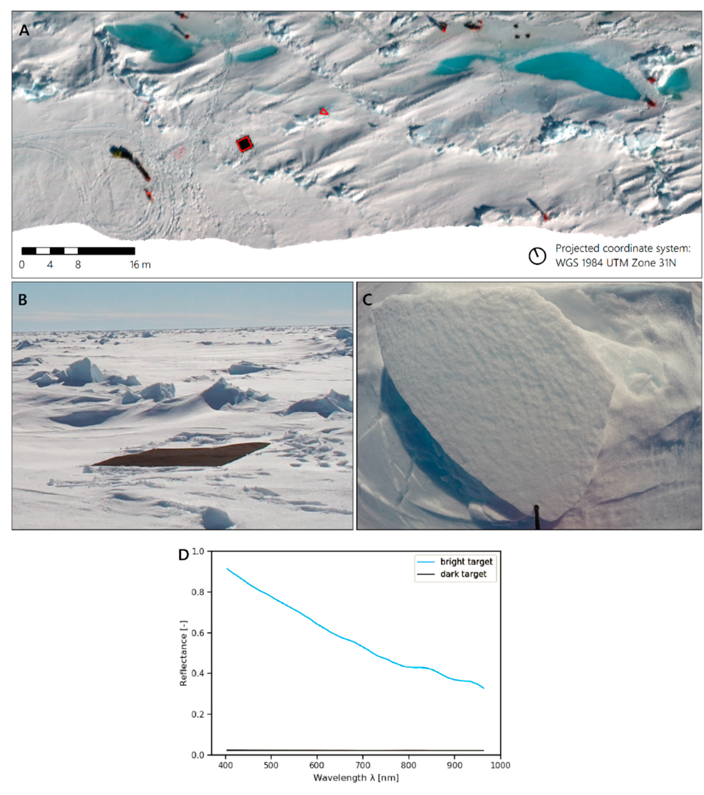
2.1.3. Spectral Reference Measurements
2.1.4. Measurements of Atmospheric Parameters
2.2. Remote-Sensing Data
Radiometric and Geometric Preprocessing
2.3. Atmospheric Correction
2.3.1. Atmospheric and Topographic Correction Version 4 (ATCOR-4)
2.3.2. Empirical Line Calibration
2.4. Retrieval of Melt Pond Depth
2.5. Evaluation
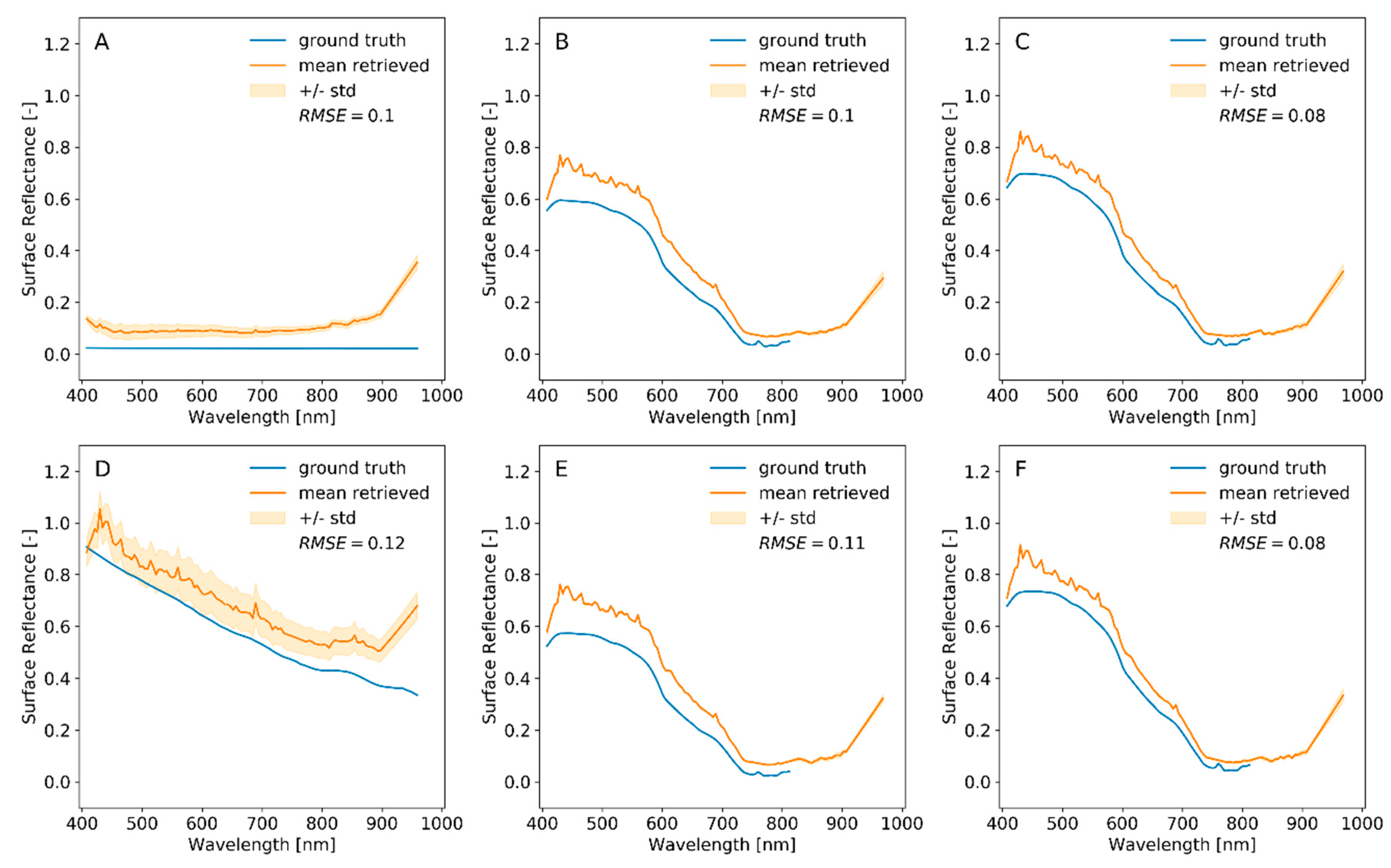
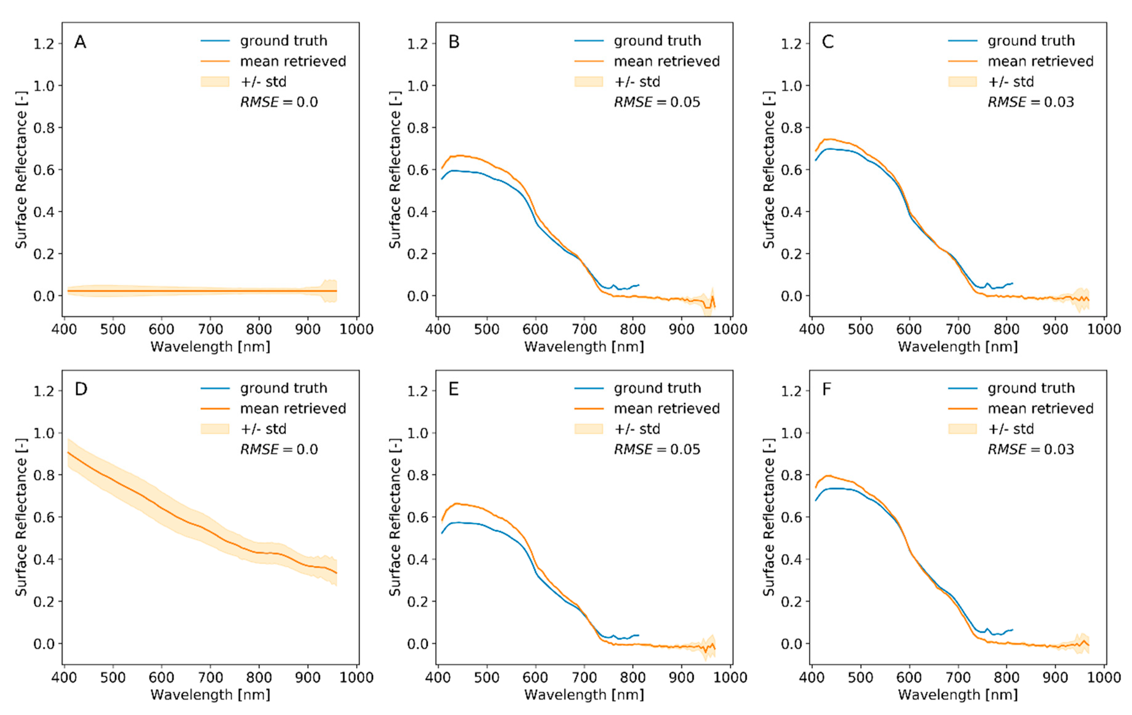
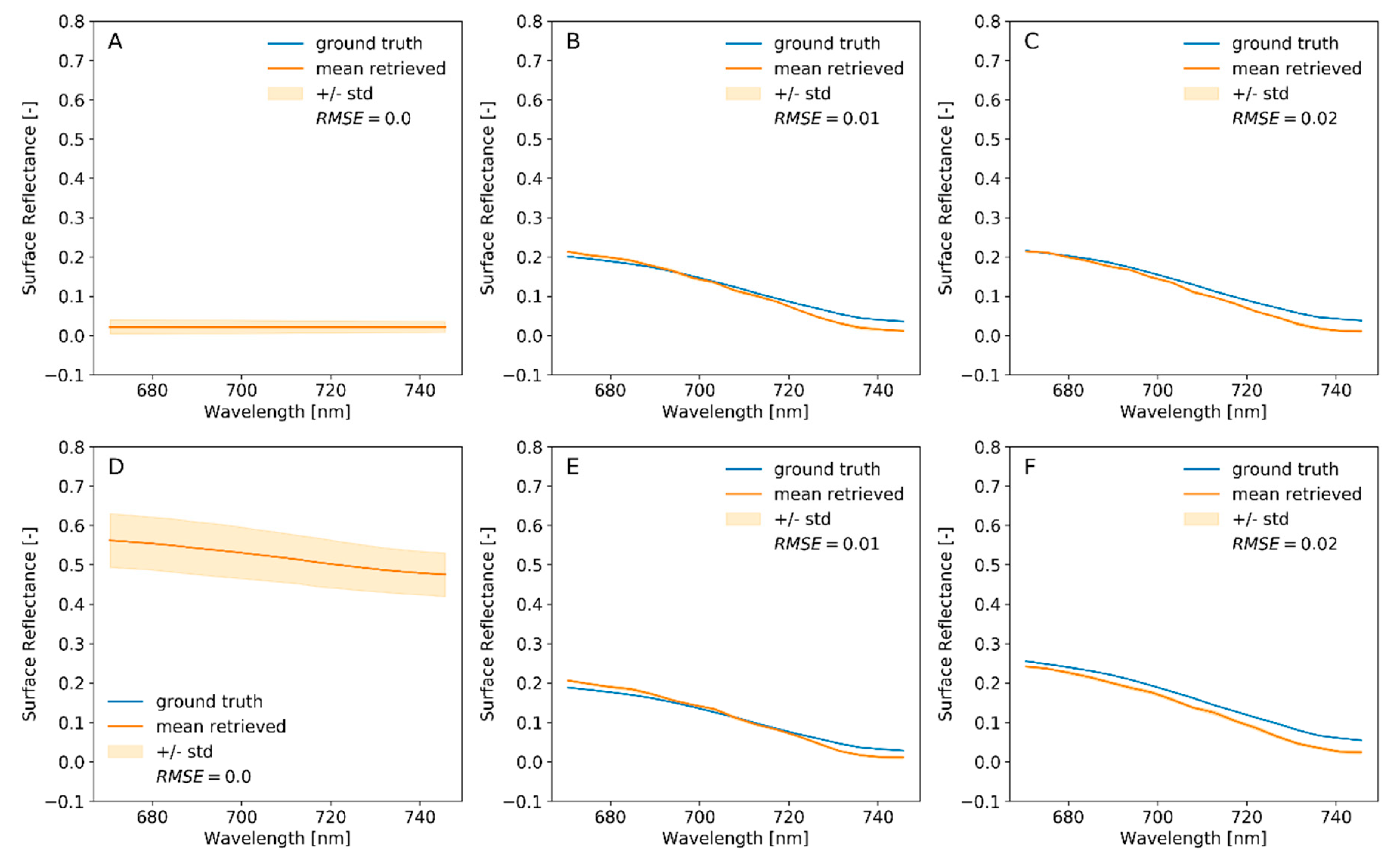
2.5.1. Evaluation of Atmospheric Correction
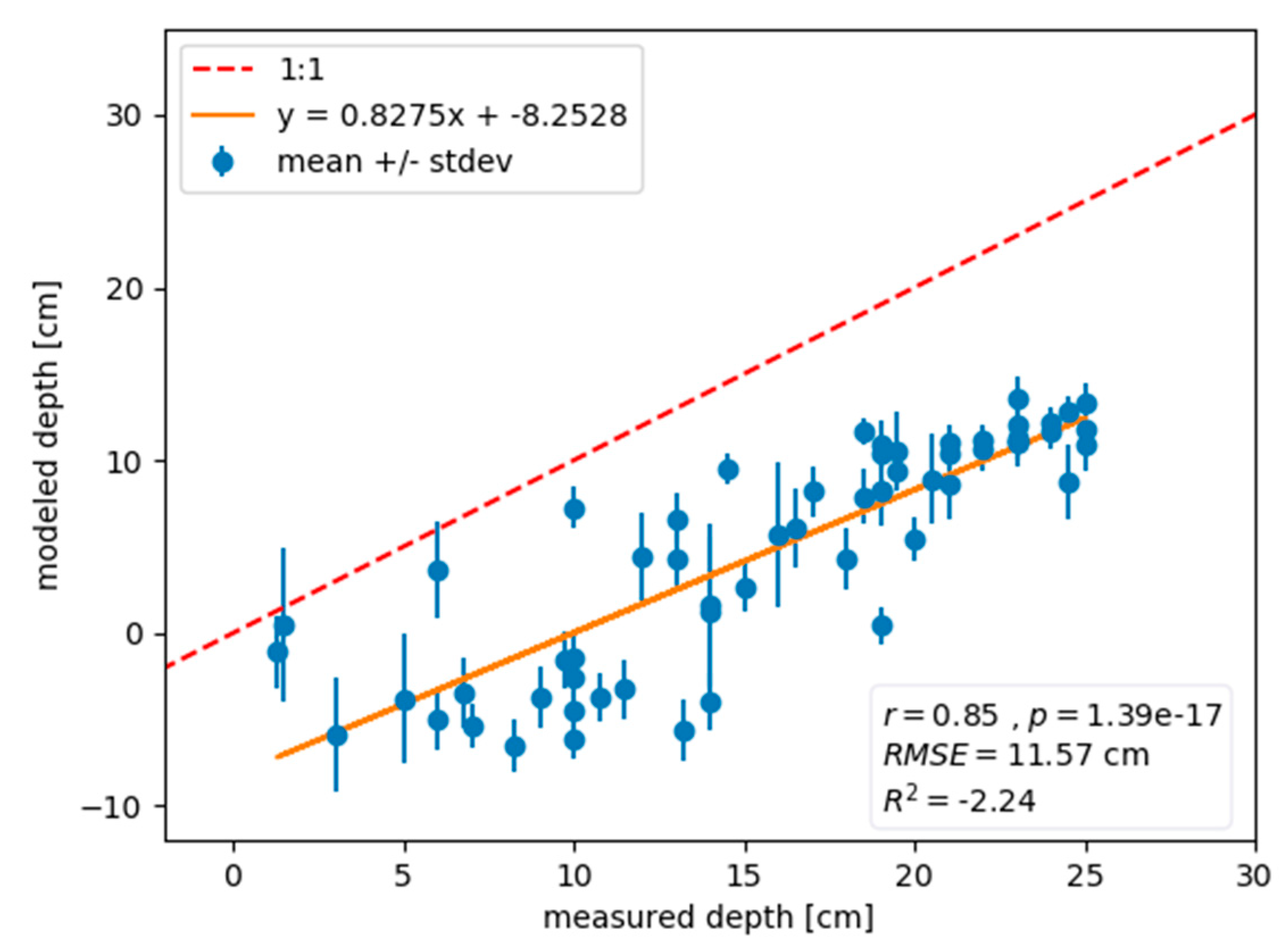
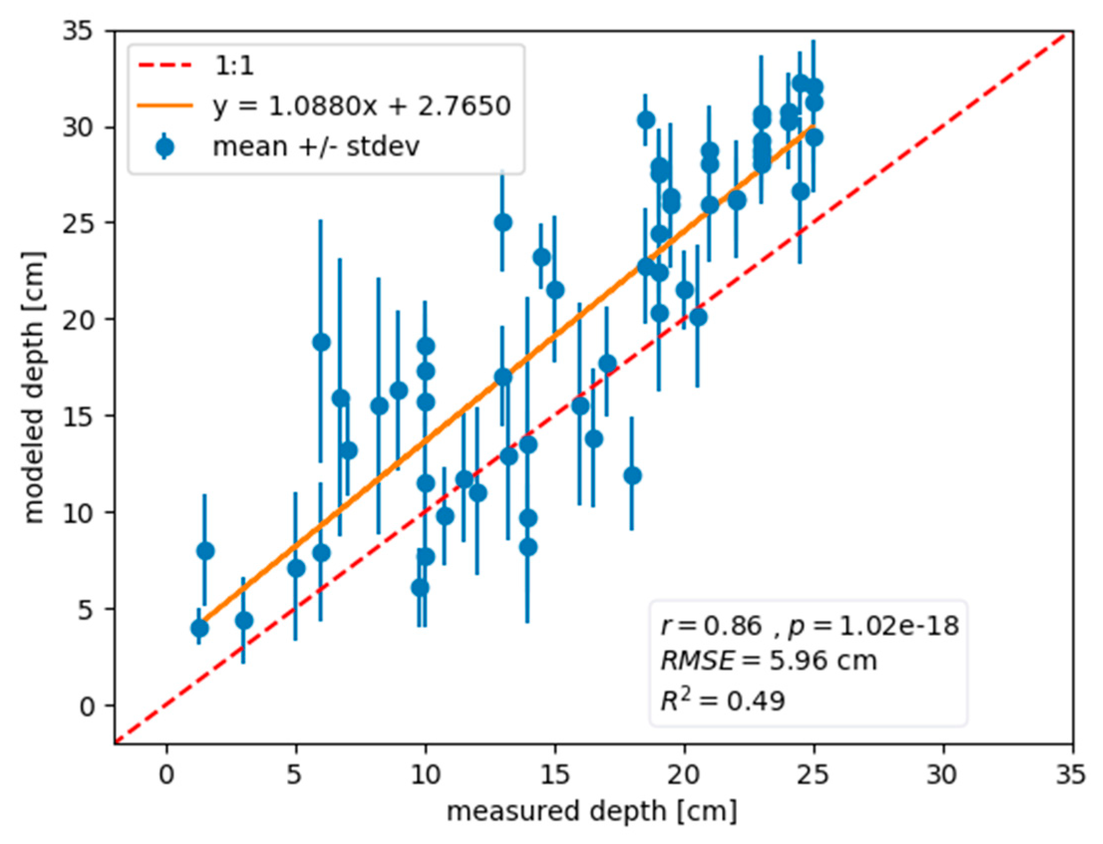
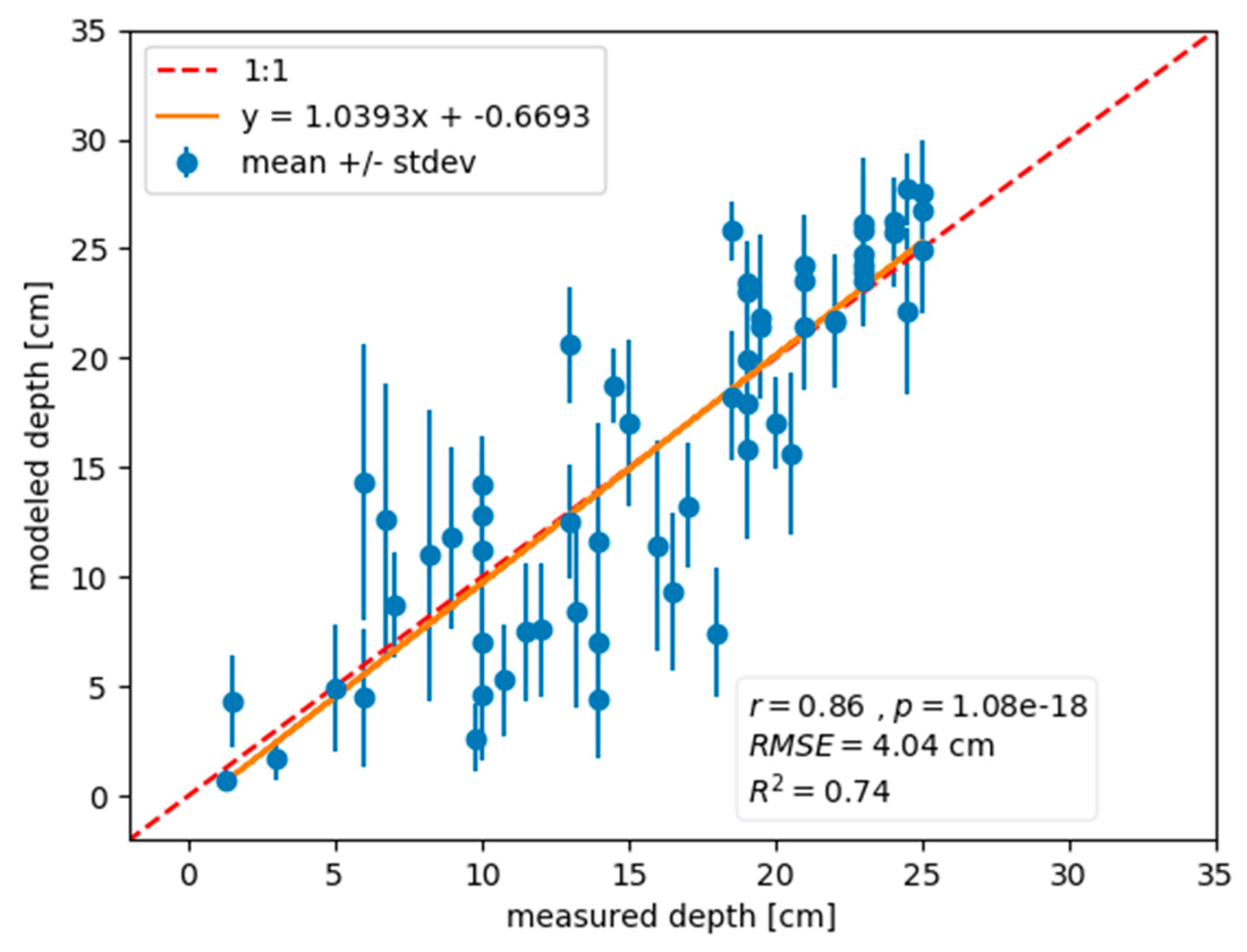
2.5.2. Evaluation of Bathymetry Retrieval
3. Results
3.1. ATCOR-4
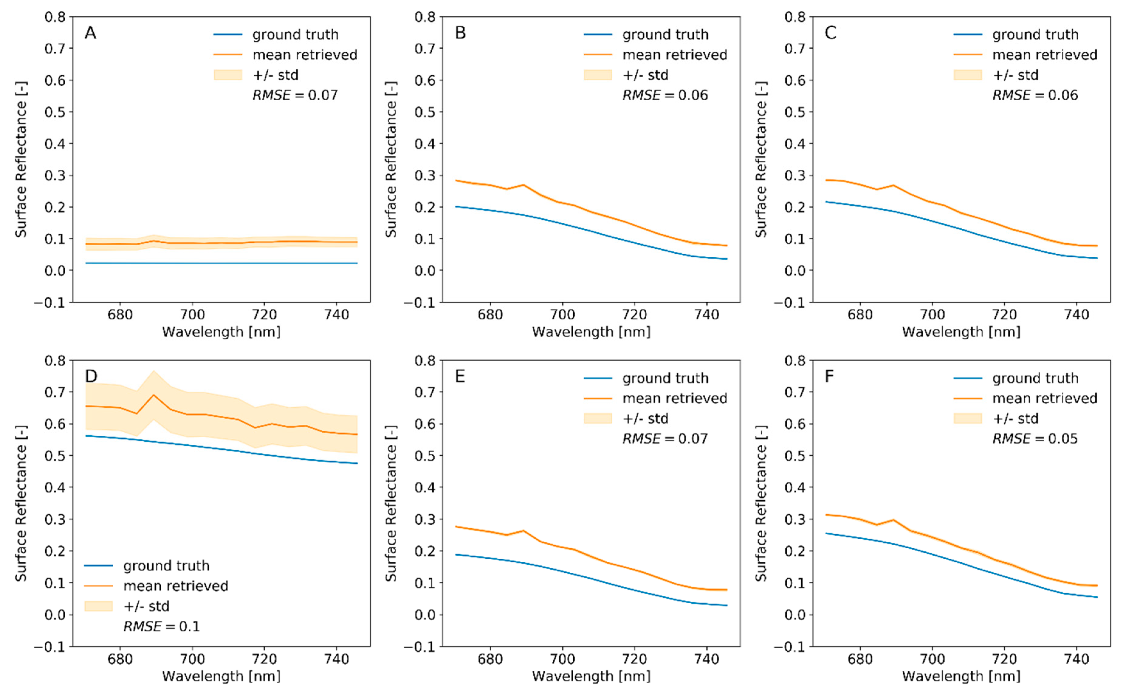
3.2. Empirical Line Calibration
4. Discussion
4.1. ATCOR-4
4.2. Empirical Line Calibration
4.3. Pond Depth Retrieval
4.4. Spatial Uncertainties
5. Conclusions
Author Contributions
Funding
Acknowledgments
Conflicts of Interest
References
- Taylor, P.D. A model of melt pond evolution on sea ice. J. Geophys. Res. 2004, 109, C12007. [Google Scholar] [CrossRef]
- Curry, J.A.; Schramm, J.L.; Ebert, E.E. Sea Ice-Albedo Climate Feedback Mechanism. J. Clim. 1995, 8, 240–247. [Google Scholar] [CrossRef]
- Kwok, R.; Untersteiner, N. The thinning of Arctic sea ice. Phys. Today 2011, 64, 36–41. [Google Scholar] [CrossRef]
- Arrigo, K.R.; Perovich, D.K.; Pickart, R.S.; Brown, Z.W.; van Dijken, G.L.; Lowry, K.E.; Mills, M.M.; Palmer, M.A.; Balch, W.M.; Bahr, F.; et al. Massive Phytoplankton Blooms Under Arctic Sea Ice. Science 2012, 336, 1408. [Google Scholar] [CrossRef] [PubMed]
- Light, B.; Perovich, D.K.; Webster, M.A.; Polashenski, C.; Dadic, R. Optical properties of melting first-year Arctic sea ice. J. Geophys. Res. Oceans 2015, 120, 7657–7675. [Google Scholar] [CrossRef]
- Nicolaus, M.; Katlein, C.; Maslanik, J.; Hendricks, S. Changes in Arctic sea ice result in increasing light transmittance and absorption. Geophys. Res. Lett. 2012, 39, 1–6. [Google Scholar] [CrossRef]
- Ehn, J.K.; Mundy, C.J.; Barber, D.G.; Hop, H.; Rossnagel, A.; Stewart, J. Impact of horizontal spreading on light propagation in melt pond covered seasonal sea ice in the Canadian Arctic. J. Geophys. Res. 2011, 116, C00G02. [Google Scholar] [CrossRef]
- Horvat, C.; Jones, D.R.; Iams, S.; Schroeder, D.; Flocco, D.; Feltham, D. The frequency and extent of sub-ice phytoplankton blooms in the Arctic Ocean. Sci. Adv. 2017, 3, e1601191. [Google Scholar] [CrossRef]
- Inoue, J.; Kikuchi, T.; Perovich, D.K. Effect of heat transmission through melt ponds and ice on melting during summer in the Arctic Ocean. J. Geophys. Res. Oceans 2008, 113, 1–13. [Google Scholar] [CrossRef]
- Perovich, D.K.; Polashenski, C. Albedo evolution of seasonal Arctic sea ice. Geophys. Res. Lett. 2012, 39, 1–6. [Google Scholar] [CrossRef]
- Nicolaus, M.; Gerland, S.; Hudson, S.R.; Hanson, S.; Haapala, J.; Perovich, D.K. Seasonality of spectral albedo and transmittance as observed in the Arctic Transpolar Drift in 2007. J. Geophys. Res. Oceans 2010, 115, 1–21. [Google Scholar] [CrossRef]
- Eicken, H.; Grenfell, T.C.; Perovich, D.K.; Richter-Menge, J.A.; Frey, K. Hydraulic controls of summer Arctic pack ice albedo. J. Geophys. Res. Oceans 2004, 109, C08007. [Google Scholar] [CrossRef]
- Perovich, D.K.; Tucker, W.B.; Ligett, K.A. Aerial observations of the evolution of ice surface conditions during summer. J. Geophys. Res. 2002, 107, 8048. [Google Scholar] [CrossRef]
- Webster, M.A.; Rigor, I.G.; Perovich, D.K.; Richter-Menge, J.A.; Polashenski, C.M.; Light, B. Seasonal evolution of melt ponds on Arctic sea ice. J. Geophys. Res. Oceans 2015, 120, 5968–5982. [Google Scholar] [CrossRef]
- Morassutti, M.P.; Ledrew, E.F. Albedo and depth of melt ponds on sea-ice. Int. J. Clim. 1996, 16, 817–838. [Google Scholar] [CrossRef]
- Yackel, J.J.; Barber, D.G.; Hanesiak, J.M. Melt ponds on sea ice in the Canadian Archipelago: 1. Variability in morphological and radiative properties. J. Geophys. Res. 2000, 105, 22049. [Google Scholar] [CrossRef]
- Fetterer, F.; Untersteiner, N. Observations of melt ponds on Arctic sea ice. J. Geophys. Res. Oceans 1998, 103, 24821–24835. [Google Scholar] [CrossRef]
- Serreze, M.C.; Holland, M.M.; Stroeve, J. Perspectives on the Arctic’s Shrinking Sea—Ice Cover. Science 2007, 315, 1533–1536. [Google Scholar] [CrossRef]
- Comiso, J.C. Large decadal decline of the arctic multiyear ice cover. J. Clim. 2012, 25, 1176–1193. [Google Scholar] [CrossRef]
- Kwok, R.; Cunningham, G.F.; Wensnahan, M.; Rigor, I.; Zwally, H.J.; Yi, D. Thinning and volume loss of the Arctic Ocean sea ice cover: 2003–2008. J. Geophys. Res. Oceans 2009, 114, 1–16. [Google Scholar] [CrossRef]
- Maslanik, J.; Stroeve, J.; Fowler, C.; Emery, W. Distribution and trends in Arctic sea ice age through spring 2011. Geophys. Res. Lett. 2011, 38, 2–7. [Google Scholar] [CrossRef]
- Scharien, R.K.; Hochheim, K.; Landy, J.; Barber, D.G. First-year sea ice melt pond fraction estimation from dual-polarisation C-band SAR—Part 2: Scaling in situ to Radarsat-2. Cryosphere 2014, 8, 2163–2176. [Google Scholar] [CrossRef]
- Roeckner, E.; Mauritsen, T.; Esch, M.; Brokopf, R. Impact of melt ponds on Arctic sea ice in past and future climates as simulated by MPI-ESM. J. Adv. Model. Earth Syst. 2012, 4, 1989–1995. [Google Scholar] [CrossRef]
- Istomina, L.; Heygster, G.; Huntemann, M.; Schwarz, P.; Birnbaum, G.; Scharien, R.; Polashenski, C.; Perovich, D.; Zege, E.; Malinka, A.; et al. Melt pond fraction and spectral sea ice albedo retrieval from MERIS data—Part 1: Validation against in situ, aerial, and ship cruise data. Cryosphere 2015, 9, 1551–1566. [Google Scholar] [CrossRef]
- Rösel, A.; Kaleschke, L.; Birnbaum, G. Melt ponds on Arctic sea ice determined from MODIS satellite data using an artificial neural network. Cryosphere 2012, 6, 431–446. [Google Scholar] [CrossRef]
- Tschudi, M.A.; Maslanik, J.A.; Perovich, D.K. Derivation of melt pond coverage on Arctic sea ice using MODIS observations. Remote Sens. Environ. 2008, 112, 2605–2614. [Google Scholar] [CrossRef]
- Markus, T.; Cavalieri, D.J.; Tschudi, M.A.; Ivanoff, A. Comparison of aerial video and Landsat 7 data over ponded sea ice. Remote Sens. Environ. 2003, 86, 458–469. [Google Scholar] [CrossRef]
- Markus, T.; Cavalieri, D.J.; Ivanoff, A. The potential of using Landsat 7 ETM+ for the classification of sea-ice surface conditions during summer. Ann. Glaciol. 2002, 34, 415–419. [Google Scholar] [CrossRef][Green Version]
- König, M.; Hieronymi, M.; Oppelt, N. Application of Sentinel-2 MSI in Arctic Research: Evaluating the Performance of Atmospheric Correction Approaches Over Arctic Sea Ice. Front. Earth Sci. 2019, 7, 1–18. [Google Scholar] [CrossRef]
- Wright, N.C.; Polashenski, C.M. Open-source algorithm for detecting sea ice surface features in high-resolution optical imagery. Cryosphere 2018, 12, 1307–1329. [Google Scholar] [CrossRef]
- Kim, D.J.; Hwang, B.; Chung, K.H.; Lee, S.H.; Jung, H.S.; Moon, W.M. Melt pond mapping with high-resolution SAR: The first view. Proc. IEEE 2013, 101, 748–758. [Google Scholar] [CrossRef]
- Hanson, K.J. The Albedo of Sea-Ice and Ice Islands in the Arctic Ocean Basin. Arctic 1961, 14, 188–196. [Google Scholar] [CrossRef]
- Holt, B.; Digby, S.A. Processes and imagery of first-year fast sea ice during the melt season. J. Geophys. Res. Oceans 1985, 90, 5045. [Google Scholar] [CrossRef]
- Tschudi, M.A.; Curry, J.A.; Maslanik, J.A. Airborne observations of summertime surface features and their effect on surface albedo during FIRE/SHEBA. J. Geophys. Res. Atmos. 2001, 106, 15335–15344. [Google Scholar] [CrossRef]
- Birnbaum, G.; Dierking, W.; Hartmann, J.; Lüpkes, C.; Ehrlich, A.; Garbrecht, T.; Sellmann, M. The Campaign MELTEX with Research Aircraft “POLAR 5” in the Arctic in 2008. Ber. Zur. Polar. Meeresforsch. Rep. Polar Mar. Res. 2009, 593, 3–85. [Google Scholar]
- Langleben, M.P. Albedo of Melting Sea Ice in the Southern Beaufort Sea. J. Glaciol. 1971, 10, 101–104. [Google Scholar] [CrossRef][Green Version]
- Tschudi, M.A.; Curry, J.A.; Maslanik, J.A. Determination of areal surface-feature coverage in the Beaufort Sea using aircraft video data. Ann. Glaciol. 1997, 25, 434–438. [Google Scholar] [CrossRef]
- El Naggar, S.; Garrity, C.; Ramseier, R.O. The modelling of sea ice melt-water ponds for the High Arctic using an Airborne line scan camera, and applied to the Satellite Special Sensor Microwave/Imager (SSM/I). Int. J. Remote Sens. 1998, 19, 2373–2394. [Google Scholar] [CrossRef]
- Tucker, W.B.; Gow, A.J.; Meese, D.A.; Bosworth, H.W.; Reimnitz, E. Physical characteristics of summer sea ice across the Arctic Ocean. J. Geophys. Res. Oceans 1999, 104, 1489–1504. [Google Scholar] [CrossRef]
- Hanesiak, J.M.; Barber, D.G.; De Abreu, R.A.; Yackel, J.J. Local and regional albedo observations of arctic first-year sea ice during melt ponding. J. Geophys. Res. 2001, 106, 1005. [Google Scholar] [CrossRef]
- Perovich, D.K.; Tucker, W.B. Arctic sea-ice conditions and the distribution of solar radiation during summer. Ann. Glaciol. 1997, 25, 445–450. [Google Scholar] [CrossRef]
- Skyllingstad, E.D.; Paulson, C.A.; Perovich, D.K. Simulation of melt pond evolution on level ice. J. Geophys. Res. Oceans 2009, 114, 1–15. [Google Scholar] [CrossRef]
- Lu, P.; Li, Z.; Cheng, B.; Lei, R.; Zhang, R. Sea ice surface features in Arctic summer 2008: Aerial observations. Remote Sens. Environ. 2010, 114, 693–699. [Google Scholar] [CrossRef]
- Huang, W.; Lu, P.; Lei, R.; Xie, H.; Li, Z. Melt pond distribution and geometry in high Arctic sea ice derived from aerial investigations. Ann. Glaciol. 2016, 57, 105–118. [Google Scholar] [CrossRef]
- Divine, D.V.; Granskog, M.A.; Hudson, S.R.; Pedersen, C.A.; Karlsen, T.I.; Divina, S.A.; Renner, A.H.H.; Gerland, S. Regional melt-pond fraction and albedo of thin Arctic first-year drift ice in late summer. Cryosphere 2015, 9, 255–268. [Google Scholar] [CrossRef][Green Version]
- Miao, X.; Xie, H.; Ackley, S.F.; Perovich, D.K.; Ke, C. Object-based detection of Arctic sea ice and melt ponds using high spatial resolution aerial photographs. Cold Reg. Sci. Technol. 2015, 119, 211–222. [Google Scholar] [CrossRef]
- Istomina, L.; Melsheimer, C.; Huntemann, M.; Nicolaus, M. Retrieval of sea ice thickness during melt season from in situ, airborne and satellite imagery. In Proceedings of the IEEE International Geoscience and Remote Sensing Symposium (IGARSS), Beijing, China, 10–15 July 2016; IEEE: New York, NY, USA, 2016; pp. 7678–7681. [Google Scholar]
- Langleben, M.P. Albedo and degree of puddling of a melting cover of sea ice. J. Glaciol. 1969, 8, 407–412. [Google Scholar] [CrossRef][Green Version]
- Derksen, C.; Piwowar, J.; LeDrew, E. Sea-ice melt-pond fraction as determined from low level aerial photographs. Arct. Alp. Res. 1997, 29, 345. [Google Scholar] [CrossRef]
- Sankelo, P.; Haapala, J.; Heiler, I.; Rinne, E. Melt pond formation and temporal evolution at the drifting station Tara during summer 2007. Polar Res. 2010, 29, 311–321. [Google Scholar] [CrossRef]
- Maslanik, J.; Curry, J.; Drobot, S.; Holland, G. Observations of sea ice using a low cost unpiloted aerial vehicle. In Ice in The Environment, Proceedings of the 16th IAHR International Symposium on Sea Ice, Dunedin, New Zealand, 2–6 December 2002; Int. Assoc. of Hydraulic Engineering and Research: Beijing, China, 2002; Volume 3, pp. 283–287. [Google Scholar]
- Inoue, J.; Curry, J.A.; Maslanik, J.A. Application of aerosondes to melt-pond observations over arctic sea ice. J. Atmos. Ocean. Technol. 2008, 25, 327–334. [Google Scholar] [CrossRef]
- Mingfeng, W.; Jie, S.U.; Tao, L.I.; Xiaoyu, W.; Qing, J.I.; Yong, C.A.O. Determination of Arctic melt pond fraction and sea ice roughness from Unmanned Aerial Vehicle (UAV) imagery. Adv. Polar Sci. 2018, 29, 181–189. [Google Scholar]
- Gaffey, C.; Bhardwaj, A. Applications of Unmanned Aerial Vehicles in Cryosphere: Latest Advances and Prospects. Remote Sens. 2020, 12, 948. [Google Scholar] [CrossRef]
- Watts, A.C.; Ambrosia, V.G.; Hinkley, E.A. Unmanned aircraft systems in remote sensing and scientific research: Classification and considerations of use. Remote Sens. 2012, 4, 1671–1692. [Google Scholar] [CrossRef]
- Ebert, E.E.; Schramm, J.L.; Curry, J.A. Disposition of solar radiation in sea ice and the upper ocean. J. Geophys. Res. 1995, 100, 15965–15975. [Google Scholar] [CrossRef]
- Ebert, E.E.; Curry, J.A. An intermediate one-dimensional thermodynamic sea ice model for investigating ice-atmosphere interactions. J. Geophys. Res. 1993, 98, 10085–10109. [Google Scholar] [CrossRef]
- Hunke, E.C.; Hebert, D.A.; Lecomte, O. Level-ice melt ponds in the Los Alamos sea ice model, CICE. Ocean. Model. 2013, 71, 26–42. [Google Scholar] [CrossRef]
- Flocco, D.; Feltham, D.L. A continuum model of melt pond evolution on Arctic sea ice. J. Geophys. Res. 2007, 112, C08016. [Google Scholar] [CrossRef]
- Scott, F.; Feltham, D.L. A model of the three-dimensional evolution of Arctic melt ponds on first-year and multiyear sea ice. J. Geophys. Res. Oceans 2010, 115, C12064. [Google Scholar] [CrossRef]
- Flocco, D.; Feltham, D.L.; Turner, A.K. Incorporation of a physically based melt pond scheme into the sea ice component of a climate model. J. Geophys. Res. 2010, 115, C08012. [Google Scholar] [CrossRef]
- Holland, M.M.; Bailey, D.A.; Briegleb, B.P.; Light, B.; Hunke, E. Improved sea ice shortwave radiation physics in CCSM4: The impact of melt ponds and aerosols on Arctic sea ice. J. Clim. 2012, 25, 1413–1430. [Google Scholar] [CrossRef]
- Pedersen, C.A.; Roeckner, E.; Lüthje, M.; Winther, J. A new sea ice albedo scheme including melt ponds for ECHAM5 general circulation model. J. Geophys. Res. 2009, 114, D08101. [Google Scholar] [CrossRef]
- Eicken, H. Structure of under-ice melt ponds in the central Arctic and their effect on, the sea-ice cover. Limnol. Oceanogr. 1994, 39, 682–693. [Google Scholar] [CrossRef]
- Divine, D.V.; Pedersen, C.A.; Karlsen, T.I.; Aas, H.F.; Granskog, M.A.; Hudson, S.R.; Gerland, S. Photogrammetric retrieval and analysis of small scale sea ice topography during summer melt. Cold Reg. Sci. Technol. 2016, 129, 77–84. [Google Scholar] [CrossRef]
- Legleiter, C.J.; Tedesco, M.; Smith, L.C.; Behar, A.E.; Overstreet, B.T. Mapping the bathymetry of supraglacial lakes and streams on the Greenland ice sheet using field measurements and high-resolution satellite images. Cryosphere 2014, 8, 215–228. [Google Scholar] [CrossRef]
- Moussavi, M.S.; Abdalati, W.; Pope, A.; Scambos, T.; Tedesco, M.; MacFerrin, M.; Grigsby, S. Derivation and validation of supraglacial lake volumes on the Greenland Ice Sheet from high-resolution satellite imagery. Remote Sens. Environ. 2016, 183, 294–303. [Google Scholar] [CrossRef]
- Tedesco, M.; Steiner, N. In-situ multispectral and bathymetric measurements over a supraglacial lake in western Greenland using a remotely controlled watercraft. Cryosphere 2011, 5, 445–452. [Google Scholar] [CrossRef]
- Untersteiner, N. On the mass and heat budget of arctic sea ice. Arch. Meteorol. Geophys. Bioklimatol. Ser. A 1961, 12, 151–182. [Google Scholar] [CrossRef]
- Lu, P.; Leppäranta, M.; Cheng, B.; Li, Z. Influence of melt-pond depth and ice thickness on Arctic sea-ice albedo and light transmittance. Cold Reg. Sci. Technol. 2016, 124, 1–10. [Google Scholar] [CrossRef]
- Lu, P.; Leppäranta, M.; Cheng, B.; Li, Z.; Istomina, L.; Heygster, G. The color of melt ponds on Arctic sea ice. Cryosphere 2018, 12, 1331–1345. [Google Scholar] [CrossRef]
- König, M.; Oppelt, N. A linear model to derive melt pond depth from hyperspectral data. Cryosph. Discuss. 2019, 2019, 1–17. [Google Scholar]
- McIntyre, M.L.; Naar, D.F.; Carder, K.L.; Donahue, B.T.; Mallinson, D.J. Coastal bathymetry from hyperspectral remote sensing data: Comparisons with high resolution multibeam bathymetry. Mar. Geophys. Res. 2006, 27, 129–136. [Google Scholar] [CrossRef]
- Legleiter, C.J.; Overstreet, B.T.; Glennie, C.L.; Pan, Z.; Fernandez-Diaz, J.C.; Singhania, A. Evaluating the capabilities of the CASI hyperspectral imaging system and Aquarius bathymetric LiDAR for measuring channel morphology in two distinct river environments. Earth Surf. Process. Landf. 2016, 41, 344–363. [Google Scholar] [CrossRef]
- Legleiter, C.J.; Roberts, D.A.; Lawrence, R.L. Spectrally based remote sensing of river bathymetry. Earth Surf. Process. Landf. 2009, 34, 1039–1059. [Google Scholar] [CrossRef]
- Giardino, C.; Bresciani, M.; Valentini, E.; Gasperini, L.; Bolpagni, R.; Brando, V.E. Airborne hyperspectral data to assess suspended particulate matter and aquatic vegetation in a shallow and turbid lake. Remote Sens. Environ. 2015, 157, 48–57. [Google Scholar] [CrossRef]
- Macke, A.; Flores, H. The Expeditions PS106/1 and 2 of the Research Vessel POLARSTERN to the Arctic Ocean in 2017. In Reports on Polar and Marine Research; Alfred Wegener Institute for Polar and Marine Research: Bremerhaven, Germany, 2018; Volume 719. [Google Scholar]
- König, M.; Oppelt, N. Optical Measurements of Bare Ice and Melt Ponds on Arctic Sea Ice Acquired During POLARSTERN Cruise PS106; PANGAEA: Bremen, Germany, 2019. [Google Scholar]
- Ocean Optics STS-VIS SPECS. Available online: https://oceanoptics.com/product/sts-vis-microspectrometer/#tab-specifications (accessed on 26 March 2019).
- Holben, B.N.; Eck, T.F.; Slutsker, I.; Tanré, D.; Buis, J.P.; Setzer, A.; Vermote, E.; Reagan, J.A.; Kaufman, Y.J.; Nakajima, T.; et al. AERONET—A federated instrument network and data archive for aerosol characterization. Remote Sens. Environ. 1998, 66, 1–16. [Google Scholar] [CrossRef]
- Specim Spectral Imaging Ltd. Available online: https://www.specim.fi/ (accessed on 7 August 2020).
- Mahiny, A.S.; Turner, B.J. A comparison of four common atmospheric correction methods. Photogramm. Eng. Remote Sens. 2007, 73, 361–368. [Google Scholar] [CrossRef]
- Kupiszewski, P.; Leck, C.; Tjernström, M.; Sjogren, S.; Sedlar, J.; Graus, M.; Müller, M.; Brooks, B.; Swietlicki, E.; Norris, S.; et al. Vertical profiling of aerosol particles and trace gases over the central Arctic Ocean during summer. Atmos. Chem. Phys. 2013, 13, 12405–12431. [Google Scholar] [CrossRef]
- Andreas, E.L.; Guest, P.S.; Persson, P.O.G.; Fairall, C.W.; Horst, T.W.; Moritz, R.E.; Semmer, S.R. Near-surface water vapor over polar sea ice is always near ice saturation. J. Geophys. Res. C Oceans 2002, 107, SHE 8-1–SHE 8-15. [Google Scholar] [CrossRef]
- Bélanger, S.; Ehn, J.K.; Babin, M. Impact of sea ice on the retrieval of water-leaving reflectance, chlorophyll a concentration and inherent optical properties from satellite ocean color data. Remote Sens. Environ. 2007, 111, 51–68. [Google Scholar] [CrossRef]
- Markelin, L.; Honkavaara, E.; Takala, T.; Schläpfer, D.; Suomalainen, J.; Pellikka, P. A Novel approach for the radiometric correction of airborne hyperspectral image data. ISPRS 2012, 3, 1451–1460. [Google Scholar]
- Berk, A.; Anderson, G.P.; Acharya, P.K.; Shettle, E.P. MODTRAN 5.2.0.0 User’s Manual; Spectral Sciences, Inc.: Burlington, MA, USA, 2008. [Google Scholar]
- Richter, R.; Schläpfer, D. Atmospheric/Topographic Correction for Airborne Imagery. In ATCOR-4 User Guide; ReSe Applications LLC: Vil, Switzerland, 2015. [Google Scholar]
- Gege, P. The water color simulator WASI: An integrating software tool for analysis and simulation of optical in situ spectra. Comput. Geosci. 2004, 30, 523–532. [Google Scholar] [CrossRef]
- Gege, P. WASI-2D: A software tool for regionally optimized analysis of imaging spectrometer data from deep and shallow waters. Comput. Geosci. 2014, 62, 208–215. [Google Scholar] [CrossRef]
- Gege, P. The Water Colour Simulator WASI. In User Manual for WASI Version 4.1; The Remote Sensing Technology Institute: Bremen, Germany, 2015. [Google Scholar]
- Pedregosa, F.; Varoquaux, G.; Gramfort, A.; Michel, V.; Thirion, B.; Grisel, O.; Blondel, M.; Prettenhofer, P.; Weiss, R.; Dubourg, V.; et al. Scikit-learn: Machine Learning in Python. J. Mach. Learn. Res. 2011, 12, 2825–2830. [Google Scholar]
- Scikit-Learn Developers. Mean Squared Error. Available online: https://scikit-learn.org/stable/modules/model_evaluation.html#mean-squared-error (accessed on 13 February 2019).
- The Scipy Community. Scipy.Stats.Pearsonr. Available online: https://docs.scipy.org/doc/scipy/reference/generated/scipy.stats.pearsonr.html (accessed on 13 February 2019).
- Kvålseth, T.O. Cautionary note about R 2. Am. Stat. 1985, 39, 279–285. [Google Scholar] [CrossRef]
- Thompson, D.R.; Seidel, F.C.; Gao, B.C.; Gierach, M.M.; Green, R.O.; Kudela, R.M.; Mouroulis, P. Optimizing irradiance estimates for coastal and inland water imaging spectroscopy. Geophys. Res. Lett. 2015, 42, 4116–4123. [Google Scholar] [CrossRef]
- Black, M.; Fleming, A.; Riley, T.; Ferrier, G.; Fretwell, P.; McFee, J.; Achal, S.; Diaz, A. On the atmospheric correction of Antarctic airborne hyperspectral data. Remote Sens. 2014, 6, 4498–4514. [Google Scholar] [CrossRef]
- Pozyx NV Pozyx. Available online: https://www.pozyx.io/ (accessed on 26 May 2020).
- Ammari, H.M. Mission-Oriented Sensor Networks and Systems: Art and Science; Studies in Systems, Decision and Control; Ammari, H.M., Ed.; Springer International Publishing: Cham, Switzerland, 2019; Volume 164, ISBN 978-3-319-92383-3. [Google Scholar]
- Knust, R.; Rex, M.; Haas, C.; Kanzow, T.; Wolf-Gladrow, D. Expeditionsprogramm PS122; MOSAiC: Bremerhaven, Germany, 2019. [Google Scholar]
- Adão, T.; Hruška, J.; Pádua, L.; Bessa, J.; Peres, E.; Morais, R.; Sousa, J. Hyperspectral imaging: A review on uav-based sensors, data processing and applications for agriculture and forestry. Remote Sens. 2017, 9, 1110. [Google Scholar] [CrossRef]
- Guanter, L.; Kaufmann, H.; Foerster, S.; Brosinsky, A.; Wulf, H.; Bochow, M.; Boesche, N.; Brell, M.; Buddenbaum, H.; Chabrillat, S.; et al. EnMAP Science Plan; EnMAP Technical Report; GFZ Data Services: Potsdam, Germany, 2016. [Google Scholar]


| Parameter | Unit | Minimum | Mean (± Standard Deviation) | Maximum |
|---|---|---|---|---|
| Aerosol optical thickness at 550 nm | [-] | 0.0217 | 0.0231 (± 0.0029) | 0.0317 |
| Angstrom Exponent (440 nm–870 nm) | [-] | 0.2168 | 1.0656 (± 0.4086) | 1.6412 |
| Water vapor | cm | 1.1066 | 1.1415 (± 0.0226) | 1.1881 |
© 2020 by the authors. Licensee MDPI, Basel, Switzerland. This article is an open access article distributed under the terms and conditions of the Creative Commons Attribution (CC BY) license (http://creativecommons.org/licenses/by/4.0/).
Share and Cite
König, M.; Birnbaum, G.; Oppelt, N. Mapping the Bathymetry of Melt Ponds on Arctic Sea Ice Using Hyperspectral Imagery. Remote Sens. 2020, 12, 2623. https://doi.org/10.3390/rs12162623
König M, Birnbaum G, Oppelt N. Mapping the Bathymetry of Melt Ponds on Arctic Sea Ice Using Hyperspectral Imagery. Remote Sensing. 2020; 12(16):2623. https://doi.org/10.3390/rs12162623
Chicago/Turabian StyleKönig, Marcel, Gerit Birnbaum, and Natascha Oppelt. 2020. "Mapping the Bathymetry of Melt Ponds on Arctic Sea Ice Using Hyperspectral Imagery" Remote Sensing 12, no. 16: 2623. https://doi.org/10.3390/rs12162623
APA StyleKönig, M., Birnbaum, G., & Oppelt, N. (2020). Mapping the Bathymetry of Melt Ponds on Arctic Sea Ice Using Hyperspectral Imagery. Remote Sensing, 12(16), 2623. https://doi.org/10.3390/rs12162623