Performance Evaluation of Spaceborne Integrated Path Differential Absorption Lidar for Carbon Dioxide Detection at 1572 nm

Abstract

As one of the most influential greenhouse gases, carbon dioxide (CO₂) has a profound impact on the global climate. The spaceborne integrated path differential absorption (IPDA) lidar will be a great sensor to obtain the columnar concentration of CO₂ with high precision. This paper analyzes the performance of a spaceborne IPDA lidar, which is part of the Aerosol and Carbon Detection Lidar (ACDL) developed in China. The line-by-bine radiative transfer model was used to calculate the absorption spectra of CO₂ and H₂O. The laser transmission process was simulated and analyzed. The sources of random and systematic errors of IPDA lidar were quantitatively analyzed. The total systematic errors are 0.589 ppm. Monthly mean global distribution of relative random errors (RREs) was mapped based on the dataset in September 2016. Afterwards, the seasonal variations of the global distribution of RREs were studied. The global distribution of pseudo satellite measurements for a 16-day orbit repeat cycle showed relatively uniform distribution over the land of the northern hemisphere. The results demonstrated that 61.24% of the global RREs were smaller than 0.25%, or about 1 ppm, while 2.76% of the results were larger than 0.75%. The statistics reveal the future performance of the spaceborne IPDA lidar.

1. Introduction

Global warming is mainly caused by the increasing anthropogenic emissions of greenhouse gases (GHGs). Scientists all over the world are taking great efforts to study the distribution characteristics of carbon dioxide (CO₂), which is one of the most important constituents of GHGs [1]. However, due to insufficient understanding of the sources and sinks distribution and spatiotemporal variation characteristics of CO₂, there is still a large uncertainty in modeling the interaction between carbon cycle and climate. Measurements of CO₂ concentration and distribution with high-precision and accuracy can help us to better understand the global carbon cycle and build a more accurate climate change forecasting model [2].

At present, passive remote sensing is the main method for global CO₂ detection, such as the ground-based Total Carbon Column Observing Network (TCCON), the Greenhouse gases Observing SATellite (GOSAT), and the Orbiting Carbon Observatory-2 (OCO-2) [3,4,5]. The passive remote sensing instruments, which include Fourier Transform Spectrometer and high-resolution grating spectrometer, measure the spectra of scattered or reflected near-infrared sunlight to retrieve the columnar concentration of CO₂ [6]. TCCON has the advantage of high measurement accuracy, which can be used as verification stations for satellite remote sensing. However, because of the rare number (23 stations in total) and uneven distribution, the sparse data is far from requirement for the retrieval of CO₂ flux worldwide [7,8]. The defect of dispersed spatial coverage of TCCON can be compensated to some extent by passive satellite remote sensing; yet the passive spaceborne sensors are vulnerable to the scattering effect of clouds and aerosols, complicated surface types, and limited by sun angle, which means severe data gaps at high latitudes and nighttime [9,10]. Therefore, the active remote sensing technique, which is mainly for differential absorption lidar (DIAL), is widely accepted as an appropriate way for atmosphere CO₂ detecting; however, DIAL suffers some limitations due to low signal-to-noise ratio (SNR) that will limit the detecting accuracy especially when applied to satellite platforms [11].

The space-borne pulsed dual-wavelength integrated path differential absorption (IPDA) lidar can not only make up the lack of passive instruments but also realize continuous day and night detection. Furthermore, the IPDA lidar can discriminate the effect of clouds and aerosols; compared to DIAL, its high signal-to-noise ratio (SNR) guarantees accurate satellite measurements [12,13]. Therefore, many research institutions have been studying and developing the space-borne IPDA lidar. In 2007, the Active Sensing of CO₂ Emissions over Nights, Days, and Seasons (ASCENDS) project was adopt by NASA [14], and NASA Goddard Space Flight Center conducted the first airborne CO₂ IPDA lidar experiment in 2008 [15,16], and several more airborne experiments were carried out based on different kinds of IPDA lidar in the following years [15,17,18], such as the pulsed and continuous wave lidar of 1.57 and 2.05 μm. The feasibility of IPDA lidar for CO₂ detection was validated, e.g., for the step-locked pulsed IPDA lidar developed by Goddard Space Flight Center, the measurement errors of airborne IPDA lidar could be less than 0.8 ppm after 10 s average compared with the in-situ instrument. In 2008, the European Space Agency also proposed a plan for global greenhouse gas (carbon dioxide and methane) detection, which was the Advanced Space Carbon and Climate Observation of Planet Earth (A-SCOPE) mission [12].

China also plans to launch a satellite with lidar payloads to detect CO₂, clouds, and aerosols in mid-2021, named the Atmospheric Environment Monitoring Satellite (AEMS). The active instrument, which is Aerosol and Carbon Detection Lidar (ACDL), is independently developed by Shanghai Institute of Optics and Fine Mechanics (SIOM), Chinese Academy of Science. ACDL combines two different types of lidar, such as IPDA lidar at 1572 nm for CO₂ detection (hereafter referred to as AC-IPDA lidar) and high spectral resolution lidar (HSRL) at 532 and 1064 nm for clouds and aerosols detection [19]. Therefore, it is necessary to evaluate the performance of AC-IPDA lidar by simulating the satellite pseudo measurements under the designed hardware parameters before the launch of AEMS.

Sensitivity analysis and simulation of pseudo measurements have been researched in order to study the characteristics of IPDA lidar. In 2008, G. Ehret et al. analyzed the systematic errors and random errors of IPDA lidar for CO₂, CH₄, and N₂O detection, which is 0.2% for CO₂, 0.4% for CH₄ at 1.6 μm, and 0.3% for N₂O at 3.9 μm [20]. In 2010, Kawa et al. conducted a simulation study to evaluate the performance of IPDA lidar for ASCENDS designed by Goddard Space Flight Center and verified that the measurement precision can reach 0.5% with existing technologies on a single 10-s (70 km) sample basis [21]. NASA Langley Research Center conducted a feasibility study of a space-based high pulse energy 2 μm CO₂ IPDA lidar, and the results showed the precision could be less than 0.35 ppm, and the accuracy was less than 0.3 ppm [22]. In 2017, Han et al. studied the feasibility and error budget of Chinese CO₂ IPDA lidar on the regional and city scale [23,24]. In 2019, Zhu et al. introduced the designed hardware system of laser transmitter and analyzed the sensitivity of an airborne IPDA lidar [25], which was a prototype of Chinese spaceborne IPDA lidar instrument.

The purpose of this study is to simulate the measurements of the spaceborne AC-IPDA lidar for CO₂ detection and to evaluate the performance accordingly. Section 2 briefly introduces the principle and the retrieval algorithm of AC-IPDA lidar, and the error analysis model is also discussed. The dataset utilized in the study is presented in Section 3, which includes satellite measurements and European Centre for Medium-Range Weather Forecasts (ECMWF) public datasets. Section 4 provides the analysis results of systematic errors and random errors and the global distribution of pseudo measurements of AEMS. In Section 5, the global results of pseudo data and seasonal variation characteristics of the random errors of AC-IPDA lidar are discussed, and concluding remarks are given in the next section.

2. Method

2.1. IPDA Lidar Principle

Spaceborne pulsed dual-wavelength IPDA lidar alternately emits two pulsed lasers near 1572 nm in a sequential manner. After being absorbed by CO₂ or other atmospheric constituents and scattered by hard targets, e.g., earth’s surface or clouds, the detector can get echo signals that contain the CO₂ concentration information in atmosphere. One of the operating wavelength near the CO₂ absorption peak is called on-line, while the reference wavelength far away from the peak is called off-line. By selecting appropriate working wavelength and taking advantage of the differential absorption effect, the influence of other trace gases and air molecules can be minimized, which means the different intensity of the echo signals is mainly caused by CO₂ in atmosphere. In the method described below, the laser is assumed to be monochromatic light. The power of lidar echo signals received by the detector can be expressed as [20].

$$\begin{array}{c}\mathrm{P}\left({\lambda }_{on,off}\right)=A·\frac{E_0\left({\lambda }_{on,off}\right)}{t_r}·\frac{{\rho }_{on,off}}{\pi }·\frac{\eta }{H_G^2}·\exp \left\{-2\left[{\tau }_{ATM}+{\tau }_{C{O}_2}\left({\lambda }_{on,off}\right)\right]\right\}\end{array}$$

(1)

where $\mathrm{P}\left({\lambda }_{on,off}\right)$ is the power of lidar echo signals, $E_0\left({\lambda }_{on,off}\right)$ is the energy of laser pulse, $\mathrm{A}$ is the area of telescope, and ${\rho }_{on,off}$ is the reflectivity of the hard targets at 1572 nm when the satellite works at nadir mode. $\mathsf{\eta }$ is the optical efficiency of the receiver system including the overlap function, $H_G$ is the altitude of the satellite platform, ${\tau }_{C{O}_2}$ and ${\tau }_{ATM}$ are the optical depth of CO₂ and other constituents in atmosphere such as H₂O, clouds, and aerosols, respectively, and $t_r$ is the effective pulse width of the echo signals, which can be expressed by [20].

$$\begin{array}{c}{t}_r=\sqrt{\Delta t_L^2+{\left(\frac{1}{3B}\right)}^2+\left(\frac{2\Delta H}{c}\right)}\end{array}$$

(2)

where $\mathsf{\Delta }{t}_L$ is the transmittance laser pulse width, $\mathrm{B}$ is the electrical bandwidth of lidar detector, $\mathsf{\Delta }\mathrm{H}$ is the surface roughness in the laser footprint, and $\mathrm{c}$ is the speed of light in vacuum.

To simulate the absorption spectra of IPDA lidar under real-world atmospheric and surface state, the absorption effect of water vapor as well as the changes of air temperature and pressure should be taken into consideration simultaneously. By simulating the absorption spectra of CO₂ molecules at different wavelengths, the CO₂ differential optical depth can be expressed as.

$$\begin{array}{c}\Delta {\tau }_{C{O}_2}=\underset{P_{TOA}}{\overset{P_{surf}}{{\displaystyle \int }}}{N}_{C{O}_2}\left(p\right)·\frac{\mathsf{\Delta }{\sigma }_{C{O}_2}\left(p\right)}{\left(m_{dryair}+m_{H_{2}O}·N_{H_{2}O}\left(p\right)\right)g}dp=\frac{1}{2}·\ln \left(\frac{P_{off}{E}_{on}}{P_{on}{E}_{off}}\right)\end{array}$$

(3)

where $\Delta {\tau }_{C{O}_2}$ is the differential optical depth,$P_{surf}$ and $P_{TOA}$are the pressure of scattering surface and the top of atmosphere (TOA), respectively, $N_{C{O}_2}\left(p\right)$ and $N_{H_{2}O}\left(p\right)$ are the volume mixing ratio of CO₂ and H₂O as a function of pressure, respectively, $\mathsf{\Delta }{\sigma }_{C{O}_2}$ is the differential absorption cross-section of CO₂, $m_{dirair}$ and $m_{H_{2}O}$ are the average mass of individual air molecule and H₂O molecule, respectively, and$\mathrm{g}$is the acceleration of gravity.

2.2. XCO₂ Retrieval Algorithm

Utilizing echo signals from IPDA lidar detector, the CO₂ differential optical depth can be calculated by means of Equation (3). The weighted average column concentration of CO₂ can be further obtained through the retrieval algorithm. It is assumed that the column CO₂ mixing ratio is uniformly distributed in the vertical atmosphere, so the weighting function can be expressed as [12].

$$\begin{array}{c}Weight Function\left(T,p\right)=\frac{\Delta {\sigma }_{C{O}_2}\left(T,p\right)}{\left(m_{dryair}+m_{H_{2}O}·N_{H_{2}O}\left(p\right)\right)g}\end{array}$$

(4)

The weighting function is mainly determined by the differential absorption cross-section of CO₂ molecule and the molecule number density of air. When the atmospheric state is constant, the shape of weighting function is only a function of laser wavelengths. Different shapes of weight functions indicate that the retrieval results of IPDA lidar have different sensitivity to each atmosphere layer. To detect the sources and sinks of CO₂, the IPDA lidar must be more sensitive to CO₂ in the lower and middle troposphere [20], which means the weighting function should have a relative larger value in low part of atmosphere.

Depending on the weighting function and differential optical depth of CO₂, the column-weighted dry air mixing ratio of CO₂ (XCO₂) is calculated as.

$$\begin{array}{c}XC{O}_2=\frac{\Delta {\tau }_{C{O}_2}}{{{\displaystyle \int }}_{P_{TOA}}^{P_{surf}}Weight Function\left(p\right)dp} \end{array}$$

(5)

which denotes the weighted averaged concentration of carbon dioxide from earth’s surface to the top of atmosphere.

2.3. Random and System Error Analysis

The performance of space-borne AC-IPDA lidar is affected by various kinds of noises [20], which can be divided into random errors and systematic errors according to the noise characteristics. By introducing the instrument model and the detector model based on the satellite platform and detector parameters of AC-IPDA lidar, their impacts on the precision of lidar detection can be quantitatively analyzed. The instrument block diagram and brief description of AC-IPDA lidar are shown in Appendix A.

The random errors can be divided into dark current noise, thermal noise, background noise, and shot noise [22,23,24,26]. The SNR is used to calculate the RREs of AC-IPDA lidar and can be expressed as follows.

$$\begin{array}{c}SN{R}_{on,off}=\frac{P_{on,off}MR}{\sqrt{B\left(2e{M}^{2}FR\left(P_{on,off}+P_{back}\right)+I_d^2\right)+\frac{B^3}{3}\left(u_{0}2\pi C\right)}}\end{array}$$

(6)

$$\begin{array}{c}{I}_d^2=I_D^2+I_0^2+\frac{4k_{B}T}{R_F}+{\left(\frac{u_0}{R_F}\right)}^2 \end{array}$$

(7)

where $P_{on,off}$ is power of echo signals at on-line or off-line, $M$is the gain of detector, $R$and$F$are the responsivity and the excess noise factor of the detector, respectively, $\mathrm{e}$ is the elementary charge,$I_D^2$ is the dark current noise density, $I_0^2$ and $u_0{}^2$ are the input current noise and the voltage noise density, respectively, of the amplifier, $k_B$ is the Boltzmann constant, $R_F$ is the feedback resistor, and $\mathrm{T}$ is the temperature of $R_F$. $P_{back}$ is the background radiation, which can be denoted from the solar light as [19].

$$\begin{array}{c}{P}_{back}=I_{Solar}·\rho ·\frac{\pi {\psi }^2{A}^2}{4}\end{array}$$

(8)

where $I_{Solar}$ is the solar background irradiance, $\mathsf{\rho }$ is the nadir surface reflectivity, $\mathsf{\psi }$is the field of view (FOV), and $\mathrm{A}$is the area of telescope. The influence of overall noises is comprehensively evaluated by computing their root mean square values, which can be expressed by [23].

$$\begin{array}{c}SNR=\frac{2\sqrt{N_{shots}}}{\sqrt{{\left(\frac{1}{SN{R}_{on}^D}\right)}^2+{\left(\frac{1}{SN{R}_{off}^D}\right)}^2+{\left(\frac{1}{SN{R}_{on}^L}\right)}^2+{\left(\frac{1}{SN{R}_{off}^L}\right)}^2}}\end{array}$$

(9)

$$\begin{array}{c}RRE=\frac{\delta \Delta {\tau }_{C{O}_2}}{\Delta {\tau }_{C{O}_2}}=\frac{1}{{\delta }_{C{O}_2}·SNR}\end{array}$$

(10)

In Equation (9), $SN{R}_{on,off}^D$ and $SN{R}_{on,off}^L$ stand for the SNR of the echo signals and the laser monitor signals, respectively. $N_{shots }$is the average times of lidar echo signals along the satellite track, which is decided by the repetition frequency of laser. Spatial resolution in the horizontal direction of AC-IPDA lidar is 50 km for the land and 100 km for the sea, and the satellite sample interval between two single points is 333 m, which means that $N_{shots}$ is 148 for the land and 296 for the sea. According to G.Ehert et al., studies show that using direct detection the influence of speckle noise for lidar signals could be neglected after averaging $N_{shots }$times [20].

The systematic error is mainly limited by the hardware performance of the lidar system, and its magnitude indicates the constant bias of the measurements, which has a monotonous global distribution [24]. According to the retrieval XCO₂ in Equation (5), the analysis of systematic error include factors that can influence the CO₂ differential optical depth in the numerator and the weighting function in the denominator. The systematic error of AC-IPDA lidar can be divided into the atmospheric state parameters, the laser transmitter, and satellite platform parameters [23,24]. It is worth noting that the influence of each factor is considered to be independent, which can be expressed by [22].

$$\begin{array}{c}RSE=\frac{\delta \Delta {\tau }_{C{O}_2}}{\Delta {\tau }_{C{O}_2}}=\frac{\left|\delta \Delta {\tau }_{C{O}_2}\left({\xi }_i\right)-\delta \Delta {\tau }_{C{O}_2}\left({\xi }_i+\Delta {\xi }_i\right)\right|}{\Delta {\tau }_{C{O}_2}\left({\xi }_i\right)}\end{array}$$

(11)

where $\Delta {\tau }_{C{O}_2 }$is the differential optical depth of CO₂, and$\delta \Delta {\tau }_{C{O}_2}$is the variation of $\Delta {\tau }_{C{O}_2}$by updating factor ${\xi }_i$, which includes transmitter and satellite platform parameters, such as the laser frequency and monitoring laser energy. The detail parameters of the AC-IPDA lidar system and the satellite platform are shown in

Table 1. Atmospheric Environment Monitoring Satellite (AEMS) platform and hardware parameters of carbon dioxide integrated path differential absorption (AC-IPDA) lidar.

Category	Parameter	Value	Unit
Satellite Platform	Orbit altitude	705	km
	Viewing mode	Nadir	-
	Spatial resolution	Land:50/Sea:100	km
Transmitter System	On-line	1572.024	nm
	Off-line	1572.085	nm
	Linewidth	50	MHz
	Pulse energy	75	mJ
	Pulse width	15	ns
	Repetition rate	20	Hz
Receiver System	Detector type	InGaAs APD	-
	Telescope diameter	1	m
	Field of view	0.2	mrad
	Optical efficiency	0.6455	-
	Digitization rate	50	MHz
	Optical filter bandwidth	0.45	nm
	Responsively	0.94	A/W
	Bandwidth	1	MHz
	Feedback resistance	1	MΩ
	Excess noise factor	3.2(@M=10)	-
	Noise equivalent power	64	fw/√Hz

as follows.

Auxiliary atmospheric state parameters include temperature, pressure, and humidity profiles, which affect the integral weighting function (IWF) in Equation (11).

$$\begin{array}{c}RSE=\frac{\Delta IWF}{IWF}=\frac{\sqrt{\Delta IW{F}_T^2+\Delta IW{F}_{X{H}_{2}O}^2+\Delta IW{F}_P^2 }}{IWF}\end{array}$$

(12)

where $IWF$ is the integral weight function, which integrates from the scattering target surface to the top of atmosphere, and $\Delta IWF$ is the bias of $IWF$ caused by the uncertainty of temperature, humidity, and pressure.

Under different atmospheric state, the molecule absorption cross-sections and the molecule number density of air are different. Therefore, the uncertainty of atmospheric state parameters will affect the distribution and the integral value of the weighting function, which lead to increasing of measurement errors.

In the simulation of AC-IPDA lidar pseudo measurements, the comprehensive effects of systematic and random errors are considered simultaneously. It is assumed that different error sources are independent of each other, and the total error can be approximated as follows according to error propagation.

$$\begin{array}{c}\frac{\Delta XC{O}_2}{XC{O}_2}=\sqrt{RR{E}^2+RS{E}^2}=\sqrt{{\displaystyle \sum }\left(\frac{\delta \Delta {\tau }_{C{O}_2}^i}{\Delta {\tau }_{C{O}_2}^i}\right)+{\displaystyle \sum }\left(\frac{\Delta IW{F}^j}{IW{F}^j}\right) }\end{array}$$

(13)

The $\Delta {\tau }_{C{O}_2}$ measurement errors contain the contribution of random errors and systemic errors. Due to the detector noise, speckle noise, and thermal noise, the SNR of detector signals is reduced, which further leads to random errors in the measured differential optical depth of CO₂. During the operation of satellite, the instability of laser frequency and energy and the non-monochromaticity of laser also cause a certain degree of uncertainty in the measurement of$\Delta {\tau }_{C{O}_2}$. Auxiliary atmospheric parameters from ECMWF are used as input in the processing of AC-IPDA lidar, it is also necessary to consider the uncertainty of temperature, pressure, and relative humidity, which can cause a deviation in the calculation of the weight function.

The time interval between on-line and off-line of AC-IPDA lidar is 200 μs. In such a short time, the atmosphere state can be assumed constant despite the movement of satellite platform. However, due to the pointing jitter of the spaceborne lidar and the high-speed movement of the satellite platform, the footprints between online and offline pulse cannot be perfectly overlapped. Considering the high CO₂ detecting precision demand in climate research, about 1 ppm, the influence of surface reflectivity gradient between online and offline pulse footprints to the random error of spaceborne IPDA lidar need further quantitative analysis. A. Amediek et al. study the airborne measurements of ground reflectance at 1.6 μm [27], and the results show that the gradients of the relative reflectivity on the small scales along the flight tracks are significantly large; however, after the measurement data being averaged, the retrieval XCO₂ error can be reduced to the allowable range due to the anticorrelation of the reflectivity gradients.

3. Dataset Screening

In this work, the measurements from Cloud-Aerosol Lidar and Infrared Pathfinder Satellite Observation (CALIPSO) are used to simulate the pseudo measurements of AEMS considering that they have nearly the same orbit characteristics and detection mode [28]. CALIPSO is a member of A-Train constellation and travels at 705 km sun-synchronous polar orbit until September 2018, which provides a global coverage between 82°N and 82°S. The orbit repeat cycle is 16 days and the equator-crossing time is about at 1:30 a.m./p.m.

In the simulation of AC-IPDA lidar echo signals, the attenuation effects of clouds and aerosols are calculated based on the observations made by Cloud-Aerosol Lidar with Orthogonal Polarization (CALIOP). The product used is CAL_LID_L2_05kmMLay, which has a spatial resolution of 5 km. The chosen time range of the dataset is from December 2015 to November 2016, as the December from previous year is included for a complete winter season. The optical depth in the product stands for the extinction degree of lasers. The latitude and longitude in the product are regarded as the pseudo measurement points of AC-IPDA lidar. The operating wavelength for cloud detection is at 532 nm. While for aerosols, there are two wavelengths: 532 nm and 1064 nm. The overall scattering effects of clouds and aerosols are taken into consideration at the same time, so the optical depth of clouds and aerosols are summed up both at 532 nm, which is regarded as the total optical depth (TOD) in the lidar equation for clouds and aerosol extinction. Although the wavelength of 532 nm is a little far away from 1572 nm, due to the measurement uncertainty of optical depth of CALIOP itself ($\pm 50\%$), the wavelength dependence of the extinction properties of clouds and aerosols can be ignored [21]. According to the RREs results shown in Section 4.2 and previous studies, the reflected lidar echo signals from the top of thick clouds ($\mathrm{OD}\ge 1$) are not considered by excluding those satellite measurements [26].

Nadir surface reflectivity for land is provided by MODIS (Terra and Aqua), which is from the Nadir BRDF-Adjusted Reflectance 16-Day Level-3 band 6 (1.64 μm) product. This product has a spatial resolution of 0.05° and only covers the land area. As for nadir surface reflectivity for the sea, the analysis data from CERA-SAT are used, which is a public dataset of ECMWF. By utilizing zonal wind speed of 10 m above sea level (U10) and Fresnel’s law of reflection, the sea surface reflectivity can be simulated at 1572 nm [29]. The surface roughness stands for the standard deviation of surface elevation in spaceborne lidar footprints, which is extracted from the Global Topographic 30 Are-Second Digital Elevation Model (GTOPO30 DEM).

The CO₂ profiles data from the Copernicus Atmosphere Monitoring Service (CAMS) GHG flux inversions dataset of ECMWF serve as the input truth-value to the line-by-line radiative transfer model. The spatial resolution of the CAMS GHG dataset is 1.875° in latitude and 3.75° in longitude, and the time resolution is 3 h. In order to simulate the lidar absorption spectra, the High Resolution Transmission (HITRAN) molecular absorption database in 2016 vision [30] and the temperature, pressure, and humidity profiles of CARE-SAT dataset in ECMWF are used. The radiative transfer model is constructed to simulate the absorption cross section and optical depth of CO₂ and H₂O.

The data used as the input of the forward model have a different spatial resolution to each other. For subsatellite points, the dataset data are interpolated to get the corresponding atmospheric state profiles or earth’s surface data as the forward model input.

In the forward model of AC-IPDA lidar, the absorption effect of H₂O molecule and the scattering effect of clouds and aerosols are taken into consideration by transforming the optical depth of each factor into the transmittance of atmosphere. The data processing scheme and framework of models are shown in Figure 1.

4. Results

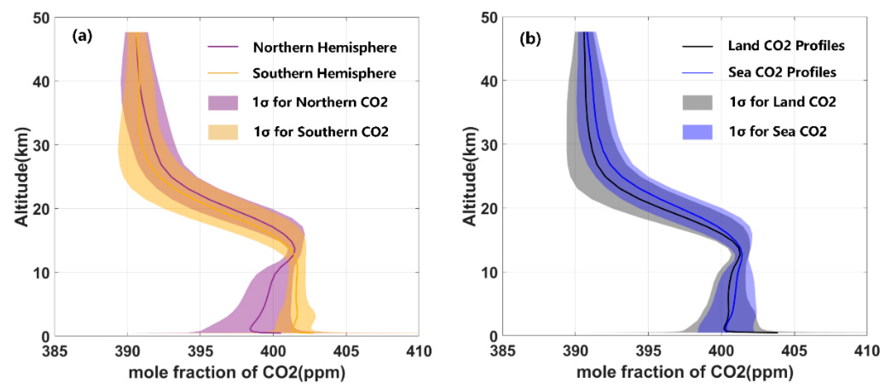
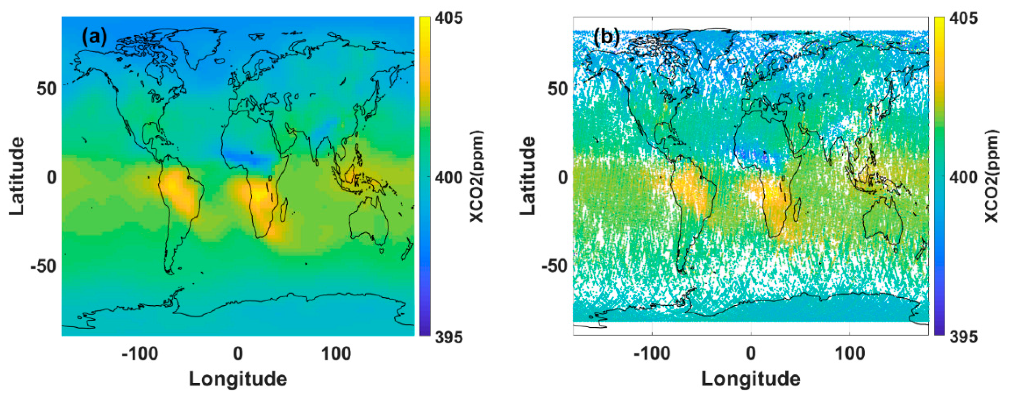
4.1. Simulation of AC-IPDA Lidar

In order to simulate the pseudo-XCO₂ data of AC-IPDA lidar, the temperature, pressure, and humidity profiles of the US 1976 standard atmospheric model and the HITRAN 2016 database are used as input to the line-by-line radiative transfer model to simulate the molecule optical depth and calculate the weighting function.

Figure 2 shows that the on-line of AC-IPDA lidar is selected in the strong absorption area of CO₂, which is 0.025 cm⁻¹ away from the absorption centerline (R18). Although the centerline of CO₂ has a stronger absorption capacity, which means a larger optical depth and smaller random error, the optical depth in the centerline of CO₂ is very sensitive to the frequency instability of laser and leads to a larger systematic error. At the same time, considering the temperature sensitivity of the CO₂ absorption spectrum and the interference from other air components, the on-line of AC-IPDA lidar have been chosen as 1572.024 nm, and the off-line is at 1572.085 nm.

As Figure 3 shows, by adjusting the TOD of the clouds and aerosols and the nadir surface reflectivity, the power of AC-IPDA lidar echo signals can be obtained under different conditions according to Equation (1). Due to the absorption spectral characteristics of CO₂ near 1572 nm, the power of echo signals in off-line is 5-7 dBm bigger than that of on-line under the same total optical depth (TOD) and nadir surface reflectivity. It is worth noting that although the orbit altitude of AEMS is 705 km and the simulation of echo signals is still under this value, the integration path of the weighting function is from the surface of hard target to 45 km when simulating the spectra of CO₂ and H₂O near 1572 nm using the line-by-line radiative transfer model. There are two reasons for this, first is that the retrieval results of echo signals from the AC-IPDA lidar are the column-weighted dry air mixing ratio of CO₂. The weighting function is almost zero in the area greater than 45 km. The second is to speed up calculations and reduce computation load.

In order to get the lidar echo signals from the simulation spectra as close as possible to the real atmosphere, various kinds of noises are added to echo signals based on the instrument model and detector model of AC-IPDA lidar. Then the global distribution of pseudo XCO₂ can be obtained by retrieving the noise-adding signals with auxiliary data.

4.2. Error Analysis Results

As shown in Section 2.3, parameters that perturb the amplitude of echo signals and the SNR could be a potential source of measurement errors. Therefore, nadir surface reflectivity and the TOD at 1572 nm are influential sources of random errors under the designed hardware parameters. From the simulation results of lidar echo signals and the SNR analysis of the detector model, the influence of each factor on the random error is quantitatively analyzed.

Figure 4 shows the theoretical RREs results of AC-IPDA lidar measurements. The attenuation effect of clouds and aerosols and the surface reflectivity both directly affect the power of the echo signals. The atmospheric transmittance decreases because of the scattering effect of clouds and aerosols, which means a weaker lidar echo signal. The intensity of the echo signal is positively relative to the surface reflectivity. While the hardware parameters remain unchanged and the detector operates in the linear region, a better SNR can be expected when the lidar echo signals are stronger. As Figure 4a shows, the RREs results are calculated under a certain atmospheric and surface state. For the typical surface reflectivity of mainland and ocean cases, which is 0.2 for the land and 0.05 for the sea, the RREs results calculated under these circumstances are 0.158% and 0.334%, respectively. In addition, the influence of laser energy and the telescope diameter on the RREs of AC-IPDA lidar are also analyzed. As Figure 4b shows, on the condition that TOD is 0.5 and surface reflectivity is 0.2, the RREs are 0.195% when the energy of laser pulse is 75 mJ and the telescope diameter is 1 m, which is given by AC-IPDA lidar hardware parameters in Table 1.

Figure 5 shows the global distribution of the monthly mean RREs in September 2016, which utilize clouds and aerosols data from CALIOP and surface state data from ECMWF datasets as input to the forward model. The time range of the satellite measurements and datasets is in September 2016, which is comprised of 433 orbits and a total of 1,087,475 soundings. Figure 5d demonstrates that 61.24% of the global RREs are smaller than 0.25%, or about 1 ppm, while 2.76% of the results are larger than 0.75%. The monthly mean global distribution of TOD is shown in Figure 4a, and the TOD between 50°S and 70°S is much larger than other places because of the high probability of clouds occurrence. The same situation also appears near the equator, and the RREs are about 0.418% in the Indonesian and the Yellow Sea of China, which is caused not only by clouds but also high aerosols loading. The laser attenuation effect in these regions is much higher than other parts of the world, which leads to a lager RREs according to Figure 5d. The values of RREs are larger in parts of Antarctica and near polar regions, especially around 100°W, which is due to the increased probability of cirrus clouds occurrence according to Vertical Feature Mask products of CALIPSO. Cirrus clouds are mainly composed of ice crystals and have a stronger absorption than water clouds, which produce larger optical depth and weaker lidar echo signals.

Global surface roughness within the satellite footprints are shown in Figure 5b. Considering the laser footprint, around 70 m to 100 m, the fluctuation of the surface elevation within the footprint could not be neglected, which has an effect of broadening the laser waveform and affecting the effective pulse width of the echo signals. An extreme case of this is in mountainous regions, such as the Himalayas in Asia, and the Cordilleran through South and North America. Figure 5d shows the RREs results in these regions are relatively large, which can reach 1% or even more.

Figure 5c presents both the land surface reflectivity, which is provided by MODIS, and the nadir ocean reflectivity, which is simulated by ECMWF datasets and Ferrell’s law of reflection. As is shown in Figure 4a, regions with high surface reflectivity have smaller RREs results. Typical regions such as the Sahara and Central Australia have a reflectivity value up to 0.7 or even 0.8, and the corresponding RREs are 0.083% and 0.079%. The ocean reflectivity is smaller but has a more uniform distribution than land, which also means a smaller standard deviation in RREs according to

Table 2. The September 2016 monthly mean RREs of AC-IPDA lidar changes with latitudes.

Latitude	Sea			Land
	RREs (%)	RREs_STD 1	Number	RREs (%)	RREs_STD	Number
70°N–85°N	0.239	0.094	289	0.230	0.100	311
50°N–70°N	0.163	0.062	183	0.260	0.181	657
30°N–50°N	0.137	0.036	371	0.256	0.39	469
0–30°N	0.181	0.101	725	0.256	0.218	475
0–30°S	0.146	0.064	825	0.171	0.098	375
30°S–50°S	0.239	0.348	647	0.203	0.109	73
50°S–70°S	0.348	0.391	703	0.295	0.358	137
70°S–85°S	0.184	0.086	68	0.253	0.175	412

¹ RREs_STD stands for the standard deviation of the RREs within the divided regions.

.

Table 2 shows the analysis results of the monthly mean RREs in September 2016, which varies with latitude. By dividing the global data into two typical topographic scenes of sea and land, it can be demonstrated that in the latitude range of 50°S–70°S, the RREs have a large value of 0.348% because of the high probability of clouds occurrence, while near the equator between 0–30°S, the RREs have a relatively small distribution, which is also consistent with Figure 5d. From the perspective of entire latitudes, the average RREs on land are larger than that on the sea, which is because of the influence of land surface roughness on echo signals. The RREs can be very large in typical mountains and areas with complex surface types, which also result in larger RREs standard deviation. As shown in the results of the northern hemisphere region in Table 2, the standard deviation of RREs is much larger than that of the same latitude of ocean.

Given seasonal variations of nadir surface reflectivity and optical depth of clouds and aerosols, it is necessary to study the seasonal global distribution characteristics of the RREs for AC-IPDA lidar. By expanding the amount of analysis data for four quarters from December 2015 to November 2016, the global seasonal RREs can be simulated, and the results are shown in Figure 6. It is worth noting that the winter season is from December 2015 to February 2016. The RREs of the northern hemisphere in winter are 0.06% larger than that in summer, which is due to the smaller nadir surface reflectivity caused by snowfall and ice, especially in Europe and the high latitudes of North America, i.e., Alaska of the USA. In South and Southeast Asia, especially in India, Thailand, Myanmar, and Indonesia, the RREs of these regions in summer and fall are 0.107% and 0.073% larger that in winter and spring, respectively, because of the high probability of clouds and aerosols occurrence.

It is worth mentioning that there is an obvious RREs boundary in the west of Asia along the 50°E longitude in summer and fall. The reason for this phenomenon is the huge difference of earth’s surface types on both sides of the RREs boundary, which is the Qinghai–Tibet Plateau and the Himalayas. At the same time, the larger TOD because of the high probability occurrence of clouds and aerosols in the Indian Peninsula and the Indo–China Peninsula also increase the RREs on the right side of the boundary in summer.

Figure 7a shows the statistical results of the RREs in four seasons, which demonstrate that about 60% of the measurements are smaller than 0.25% according to the one-year data from December 2015 to November 2016. Obvious seasonal variations of the RREs can be seen in the Amazon and South Asia according to Figure 7b. Compared to summer, the RREs are larger in winter because it is in the rainy season of the Amazon. However, it can also be seen from the comparison of Figure 7b that the RREs seasonal changes in desert areas are relatively small compared to other regions, while the RREs are always large in the terrestrial mountainous areas and high latitudes of the southern hemisphere in all of the four seasons according to Figure 6.

The results of systematic errors of AC-IPDA lidar are shown in

Table 3. Summary results of various systematic errors of AC-IPDA lidar.

Category	Parameters	Uncertainty	RSE	Errors (ppm)
Atmosphere	Temperature	1 K	0.033%	0.132
	Pressure	1 hPa	0.071%	0.284
	Humidity	10%	0.037%	0.148
Laser Transmitter	Laser Energy Fluctuation	0.05%	0.037%	0.148
	Frequency Drift	0.6 MHz	0.038%	0.152
	Spectral Purity	99.9% (0.45 nm IF)	0.079%	0.316
	Laser Linewidth	50 MHz	0.07%	0.28
Satellite Platform	Doppler Effect across track	140 μrad	0.038%	0.152
	Doppler Effect along track	1 mrad	0.0005%	0.002
	Non-overlap Footprints	25 μrad	0.006%	0.024
	Laser Path	2 m	0.01%	0.04
Total				0.589

and the detailed calculation methods are presented in Section 2.3. The value of the total systematic errors indicates the measurement accuracy of AC-IPDA lidar, which will not affect the retrieval of the flux of carbon dioxide. However, it can cause a large error in the carbon emission and absorption calculation. The main limiting factors for the systematic errors of AC-IPDA lidar, as shown in Table 3, are the uncertainty of atmospheric state parameters and the instability of systematic hardware parameters according to the total systematic errors. By improving the design of the laser and optimizing the retrieval algorithm, the systematic errors of lidar system can be further corrected, and the influence of system defects on the measurement accuracy can be reduced as much as possible. Various kinds of systematic errors can be calculated quantitatively by Equations (10) and (11), and the total systematic errors are 0.589 ppm by summing these individual results geometrically.

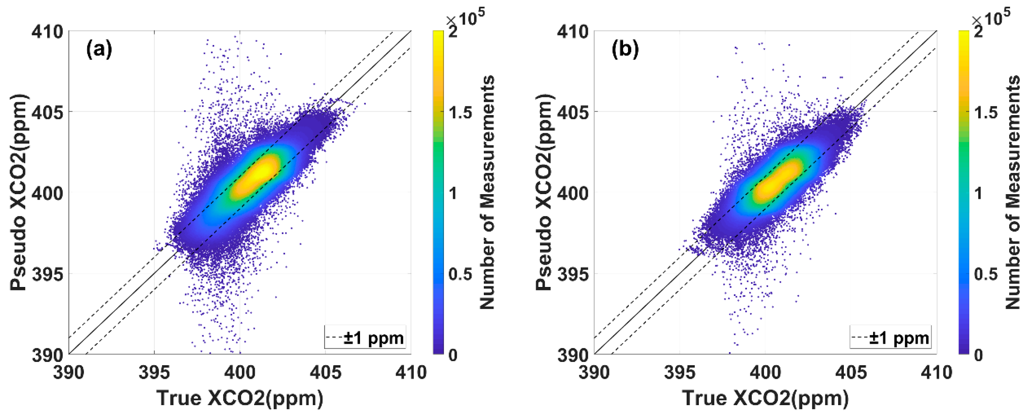
4.3. Pseudo XCO₂ of AC-IPDA Lidar

The pseudo XCO₂ data of AC-IPDA lidar are simulated based on the instrument model and detector model, which are determined by the satellite platform and the detector parameters. The line-by-line radiative transfer model is used to simulate the absorption spectra of CO₂ and H₂O under the ambient atmospheric and surface state. Then, the pseudo echo signals can be simulated by combining the ideal signals and noises. In order to retrieve the XCO₂ from the simulated lidar echo signals, the weighting function is calculated first, and the results are shown in Figure 8.

The shapes of the normalized weighting functions are shown in Figure 8, which vary with altitude and the wave number of on-line. A larger relative value of weighting function indicates that the AC-IPDA lidar is more sensitive to the atmosphere at this altitude. The detection of CO₂ sources and sinks requires that the space-borne IPDA lidar should have high sensitivity to the troposphere [12,20].

As the input of line-by-line radiative transfer model, the CO₂ profiles of CAMS GHG are first processed, and then the variations uncertainties of the CO₂ profile data in time and space (horizontal and vertical) are analyzed. The distribution characteristics of CO₂ profiles are shown in Figure 9. In Figure 9a, the dry mole fraction of CO₂ profile is significantly different below 10 km between the northern and southern hemisphere. This phenomenon is not only due to the difference in spatial location, but also for the variation in the growth of plants caused by seasonal changes. Considering the different spatial resolutions between land and sea in the operation of spaceborne AC-IPDA lidar, CO₂ profiles above the two typical subsurfaces are also analyzed respectively. The results are shown in Figure 9b. For the near ground, the dry mole fraction of CO₂ above land is greater than that on the sea, and for the CO₂ profiles with a subsurface of the sea, the standard deviation of CO₂ profiles is smaller than that on land, which may be caused by less complex surface types.

In order to study the global distribution characteristics of pseudo XCO₂ data, the clouds and aerosols data at 532 nm of CALIOP are used, which have a spatial resolution of 5 km. The collected global CALIPSO dataset in September 2016 is comprised of 233 orbits, 488,391 soundings during the day and 232 orbits, 430,640 soundings at night. The interpolated temperature, pressure, and humidity profiles of ECMWF datasets and the simulated global nadir surface reflectivity are used to match the satellite footprints. Using the matched atmospheric and earth’s surface state data as input of AC-IPDA lidar instrument and detector model, the pseudo XCO₂ data are simulated and the results are presented in Figure 9.

Figure 10 shows the global 16-day pseudo XCO₂ results of AC-IPDA lidar in September 2016. The ‘true’ XCO₂ utilizing CO₂ profiles from CAMS GHG public dataset with IPDA lidar weighting function is shown in Figure 10a. As Figure 10a shows, there is an obvious difference between the northern and the southern hemisphere because of the seasonal changes and the respiration and photosynthesis of plants. Figure 10b demonstrates that the pseudo XCO₂ has a significantly uniform distribution characteristics compared with the passive remote sensing equipment especially in high latitudes of northern hemisphere. However, the data distribution is relatively sparse between 50°S–70°S because of the high probability of clouds occurrence, and the TOD of measurements are limited to smaller than 1. According to the results in Section 4.2, this region also has larger RREs than the other ordinary parts of the world.

Figure 11 shows the simulation results of pseudo XCO₂ under the consideration of AC-IPDA lidar random errors and systematic errors simultaneously. The model XCO₂ from database represents the true value used as input into the forward model, while the longitudinal axis stands for the pseudo XCO₂, which is retrieved by simulated AC-IPDA lidar signals combined with various kinds of noises. Compared with daytime results in Figure 11a, pseudo measurement data in Figure 11b for the nighttime have a closer and denser distribution, most concentrated in the range of ±1 ppm. This phenomenon is caused by the background noise during the day. The introduction of background noise decreases the SNR of lidar return signals and increases the random errors. It is worth noting that the dispersion of diurnal pseudo data is slightly larger than night, which has a standard deviation of 0.752 ppm in the day and 0.689 ppm in the night. According to Equation (7), the field of view of the telescope is a key parameter to limit the background noise, which can effectively reduce the noise by decreasing the FOV. However, the FOV should be larger than the divergence angle of the laser beam to ensure the normal reception of lidar return signals. At present, the FOV of the telescope at AC-IPDA lidar is 0.2 mrad, while the laser divergence angle is less than or equal to 0.1 mrad, which can guarantee the normal reception of laser echo signals, reduce the background noise, and improve the SNR of echo signals as much as possible at the same time.

5. Discussion

This work evaluated the performance of spaceborne IPDA lidar and demonstrated that its measurement precision could meet the designed goals on the global scale. The forward model was simulated to study the lidar echo signals of AC-IPDA lidar, the global distribution and the seasonal variation characteristics of RREs, and the systematic errors were calculated to study the precision and accuracy the AC-IPDA lidar. Finally, the pseudo XCO₂ data were simulated by the retrieval algorithm. The results suggest that about 60% of the earth’s surface can reach the precision requirements for AC-IPDA lidar, and the pseudo measurement data displayed a global well-proportioned distribution, especially in high latitude regions.

According to the error analysis results of AC-IPDA lidar, the absorption effect of clouds and aerosols, the surface reflectivity, and the surface roughness are three important environmental factors greatly affecting the measurement precision. The advantage of IPDA lidar is its range-resolved return signals, which can diminish the interference of multiple scattering effects of clouds and aerosols with a definite lidar optical path. However, the attenuation effects of clouds and aerosols still have a profound impact on the measurement precision, especially in areas with heavy aerosols loading and high possibility of cloud occurrence. Therefore, the results suggest that the measurement precision of East Asia, Southeast Asia, tropical regions, and high latitude regions of the southern hemisphere is not very optimistic. Similar results were also studied by Ge Han et al. [23,24], which demonstrated that for many metropolitan cities in China, especially in the eastern coastal regions, the measurement precision would decrease because of heavy air pollution and high aerosol loading.

The impact of clouds on spaceborne IPDA lidar are more complicated than aerosols. Different types of clouds have different effects on lidar signals [31]. The detector of AC-IPDA lidar can receive return signals from the top of clouds when the cloud thickness and surface reflectivity are large enough, and then the partial column XCO₂ can be retrieved [32]. The influence factor of clouds on lidar signals are surface roughness, surface reflectivity, cloud top height, and cloud thickness. These properties are closely related to the types of clouds. For example, the surface reflectivity of stratus and cumulus can reach 0.05 at 1572 nm, which can be used as hard scattering targets for IPDA lidar; however, cirrus clouds are usually thin and semi-transparent, and the strong absorption effect leads to a rather smaller surface reflectivity less than or equal to 0.01 [33]. Consequently, the SNR of lidar signals will decrease in the presence of cirrus clouds, which is not conducive to further data processing. It is difficult to obtain high-precision cloud types, distribution, and physical characteristics data as input to the forward model. Therefore, we only consider the absorption effect of clouds on lidar return signals in this work and average echo signals within every 50 km $\times$ 50 km grid. However, it should be pointed out that during the operation of AC-IPDA lidar, the partial column XCO₂ from clouds tops can be retrieved when the SNR of return signals are sufficient. Considering the wide spatial distribution, the variety of types and physical properties of clouds have great impact on lidar signals, and further ground-based and airborne experiments, verification, and sensitivity tests are required to evaluate the performance of AC-IPDA lidar under complex clouds scenarios.

The uncertainty of auxiliary data and the instability of laser parameters are the main factors that affect the systematic errors, and the results show the total systematic errors are 0.589 ppm. The analysis result is about 0.2 ppm larger compared with previous sensitivity studies of spaceborne IPDA lidar [20]. This is caused by a variety of reasons, such as differences in the version of HITRAN database used for the forward model and the design parameters of lidar, which include the wavelength of lidar, orbit parameters of satellite, etc. The systematic errors of AC-IPDA lidar will lead to deviations of absolute value in the estimation of the sources and sinks of CO₂, which will further affect the carbon–climate intersection model forecasting. Although kinds of systematic errors can be corrected by calibration experiments, there are still strict requirements for the stability of AC-IPDA lidar. The atmosphere auxiliary data are used to calculate the air number density, and the uncertainty of auxiliary data directly affect the measurement accuracy of AC-IPDA lidar. In addition, the current atmospheric auxiliary data in public databases are simulated values that unidirectionally change with altitude or pressure; however, the variations in terrain areas with complex surface types such as in the mountains are more complicated, and the reanalysis atmospheric auxiliary data need further optimization.

The satellite simulation pseudo dataset results show that the measurement data of spaceborne AC-IPDA lidar are evenly distributed worldwide, especially in the high latitudes near the polar regions. Factors that affect the high-quality measurement distribution of AC-IPDA lidar include not only the spatial characteristics of clouds and aerosols but also the surface types. For the earth’s surface, the variation of surface reflectivity and the surface roughness in complex surface areas both have significant impacts on lidar signals, especially in the mountains. Therefore, the signal processing and quality control algorithm need further research and development.

The comparisons between simulated pseudo XCO₂ and ground-based and airborne validation experiments also show a good consistency. In 2017, Du et al. carried out the ground validation experiment of IPDA lidar utilizing a wall as a reflected hard target that was 1.17 km away [34]. XCO₂ data were measured in the limited path and compared with the measurement data of an in situ ultraportable greenhouse gas analyzer (UGGA). The results show that the XCO₂ is 432.71 $\pm$ 2.42 ppm after 18 s average (900 shots), and the accuracy is 0.56%. In March 2019, the prototype of AC-IPDA lidar developed by SIOM carried out an airborne verification experiment in Shanhaiguan, China. According to the study of Zhu et al. [35], the airborne results show that in a calm sea area that is 30 km away from the coast without drastic changes in CO₂ sources and sinks, the IPDA lidar measurement result is 414.69 ppm, the standard deviation is 1.02 ppm, and the accuracy is 0.246%. The measurement results of in situ instruments in the same period is 413.39 ppm. The bias between IPDA lidar and in situ instruments is 1.30 ppm, which means an accuracy of 0.313%. The satellite simulation pseudo dataset results show that the global 16-day averaged measurement precision is 0.752 ppm in the daytime and 0.689 ppm in the nighttime, and the precision in a single day ranges from 0.8 to 1.5 ppm. Considering the updated IPDA lidar hardware system and the different ambient environment, the difference of results is within an acceptable range.

It is worth noting that some assumptions are taken to facilitate evaluation of the performance of AC-IPDA lidar. Firstly, only the attenuation effect of clouds when total optical depth was smaller than 1 was taken into consideration, and the lidar echo signals that reflected from the top of dense and thick clouds were excluded. Removing such scenarios, on the other hand, would significantly decrease the effective coverage of earth’s surface for satellite measurement data. Regarding the impact of the surface roughness on pseudo data simulation of AC-IPDA lidar, we only consider elevation fluctuations in the laser footprint. The impacts of different surface types have not been further analyzed. Finally, considering the payloads of AEMS include an HSRL that measures the clouds and aerosols simultaneously with IPDA lidar, an innovative retrieval algorithm to improve the measurement accuracy and precision of AC-IPDA lidar by assimilating the data from HSRL requires further study, which will be our next stage of work.

6. Conclusions

In this paper, the performance of a newly designed space-borne IPDA lidar, AC-IPDA lidar, was evaluated by analyzing the detection uncertainty of the column-weighted dry air mixing ratio of CO₂. The line-by-line radiative transfer model based on HITRAN 2016 was first constructed to calculate the absorption spectra of CO₂ and H₂O, then the pseudo echo signals were simulated by introducing the instrument model and detector model, which were based on satellite platform and detector parameters. The meteorological data from ECMWF datasets and satellite measurements were used to simulate the ambient atmospheric and surface condition.

The power and various kinds of errors in AC-IPDA lidar pseudo echo signals were simulated for different surface reflectivity and TOD with the 1976 US standard atmosphere model. The RREs were 0.158% for general land and 0.334% for ocean when the surface reflectivity was 0.2 sr⁻¹ and 0.05 sr⁻¹, respectively. The influence of the telescope aperture and the pulse laser energy on RREs were also analyzed. The total systematic errors were 0.589 ppm, which demonstrated that the designed system stability could meet the measurement precision requirements.

The global distribution characteristics of monthly mean RREs were analyzed based on the dataset in September 2016, demonstrating that 61.24% of the global RREs could be expected to reach the designed accuracy standard of the RREs less than 0.25%, about 1 ppm, while only 2.76% of the results were larger than 0.75%. The areas with larger RREs were mainly due to four reasons: (1) topography in mountainous regions such as the Himalayas, (2) high probability of clouds occurrence within the latitudes between 50°S–70°S, (3) high aerosol loadings, and (4) mixed surface types of land and water, i.e., in the south of Asia, the Yellow Sea of China, and Indonesia, had a larger RREs of 0.418%. Thus, apart from clouds and aerosols, which were indeed important factors affecting the distribution of the RREs of AC-IPDA lidar, the influence of surface roughness could not be ignored.

The analysis of the RREs results in different seasons demonstrated that about 60% of the global RREs were smaller than 0.25% based on the one-year dataset. At the same time, a seasonal variation characteristic of the RREs of AC-IPDA lidar was founded due to the changes in surface reflectivity and occurrence frequency of clouds and aerosols. In general, the RREs of the northern hemisphere in winter and spring were larger than that in summer and fall. Compared to other regions in the world, the seasonal variations of RREs were most obvious in the Amazon and South Asia, while there were no significant changes in desert areas such as Sahara and Central Australia.

The pseudo XCO₂ data had a uniform global distribution especially in the high-latitude regions of the northern hemisphere during both day and night. The standard deviation between the model true value and the pseudo XCO₂ data of AC-IPDA lidar is 0.752 ppm during the day, while the value at night was 0.689 ppm. In other words, measurements at night without solar background noise could have a better performance than that during the day. In general, the measurement precision of AC-IPDA lidar can meet the design requirements both in daytime and nighttime conditions.

References

1. IPCC. Climate Change 2013—The Physical Science Basis: Working Group I Contribution to the Fifth Assessment Report of the Intergovernmental Panel on Climate Change; Stocker, T.F., Qin, D., Plattner, G.-K., Tignor, M., Allen, S.K., Boschung, J., Nauels, A., Xia, Y., Bex, V., Midgley, P.M., Eds.; Cambridge University Press: Cambridge, UK, 2014; p. 1535. [Google Scholar]
2. Friedlingstein, P.; Cox, P.; Betts, R.; Bopp, L.; von Bloh, W.; Brovkin, V.; Cadule, P.; Doney, S.; Eby, M.; Fung, I.; et al. Climate–Carbon Cycle Feedback Analysis: Results from the C4MIP Model Intercomparison. J. Clim. 2006, 19, 3337–3353. [Google Scholar] [CrossRef]
3. Crisp, D.; Team, O.C.O. Measuring Atmospheric Carbon Dioxide from Space with the Orbiting Carbon Observatory-2 (OCO-2). In Proceedings of the SPIE Optical Engineering + Applications, San Diego, CA, USA, 9–13 August 2015. [Google Scholar]
4. Wunch, D.; Toon, G.C.; Blavier, J.F.L.; Washenfelder, R.A.; Notholt, J.; Connor, B.J.; Griffith, D.W.T.; Sherlock, V.; Wennberg, P.O. The Total Carbon Column Observing Network. Philos. Trans. R. Soc. A Math. Phys. Eng. Sci. 2011, 369, 2087–2112. [Google Scholar] [CrossRef] [PubMed] [Green Version]
5. Kuze, A.; Suto, H.; Shiomi, K.; Kawakami, S.; Tanaka, M.; Ueda, Y.; Deguchi, A.; Yoshida, J.; Yamamoto, Y.; Kataoka, F.; et al. Update on GOSAT TANSO-FTS performance, operations, and data products after more than 6 years in space. Atmos. Meas. Tech. 2016, 9, 2445–2461. [Google Scholar] [CrossRef] [Green Version]
6. O’Dell, C.W.; Connor, B.; Boesch, H.; O’Brien, D.; Frankenberg, C.; Castano, R.; Christi, M.; Eldering, D.; Fisher, B.; Gunson, M.; et al. The ACOS CO2 retrieval algorithm—Part 1: Description and validation against synthetic observations. Atmos. Meas. Tech. 2012, 5, 99–121. [Google Scholar] [CrossRef] [Green Version]
7. Gurney, K.R.; Law, R.M.; Denning, A.S.; Rayner, P.J.; Baker, D.; Bousquet, P.; Bruhwiler, L.; Chen, Y.-H.; Ciais, P.; Fan, S.; et al. Towards robust regional estimates of CO2 sources and sinks using atmospheric transport models. Nature 2002, 415, 626–630. [Google Scholar] [CrossRef] [Green Version]
8. Bruhwiler, L.M.P.; Michalak, A.M.; Tans, P.P. Spatial and temporal resolution of carbon flux estimates for 1983–2002. Biogeosciences 2011, 8, 1309–1331. [Google Scholar] [CrossRef]
9. Houweling, S.; Hartmann, W.; Aben, I.; Schrijver, H.; Skidmore, J.; Roelofs, G.J.; Breon, F.M. Evidence of systematic errors in SCIAMACHY-observed CO2 due to aerosols. Atmos. Chem. Phys. 2005, 5, 3003–3013. [Google Scholar] [CrossRef] [Green Version]
10. Buchwitz, M.; de Beek, R.; Burrows, J.P.; Bovensmann, H.; Warneke, T.; Notholt, J.; Meirink, J.F.; Goede, A.P.H.; Bergamaschi, P.; Korner, S.; et al. Atmospheric methane and carbon dioxide from SCIAMACHY satellite data: Initial comparison with chemistry and transport models. Atmos. Chem. Phys. 2005, 5, 941–962. [Google Scholar] [CrossRef] [Green Version]
11. Han, G.; Gong, W.; Lin, H.; Ma, X.; Xiang, Z.C. Study on Influences of Atmospheric Factors on Vertical CO2 Profile Retrieving From Ground-Based DIAL at 1.6 mu m. IEEE Trans. Geosci. Remote Sens. 2015, 53, 3221–3234. [Google Scholar] [CrossRef]
12. Caron, J.; Durand, Y.; Bezy, J.-L.; Meynart, R. Performance Modeling for A-SCOPE: A Space-Borne Lidar Measuring Atmospheric CO2; SPIE Remote Sensing: Edinburgh, UK, 2009; Volume 7479. [Google Scholar]
13. Ehret, G.; Bousquet, P.; Pierangelo, C.; Alpers, M.; Millet, B.; Abshire, J.B.; Bovensmann, H.; Burrows, J.P.; Chevallier, F.; Ciais, P.; et al. MERLIN: A French-German Space Lidar Mission Dedicated to Atmospheric Methane. Remote Sens. 2017, 9, 1052. [Google Scholar] [CrossRef] [Green Version]
14. NTRS-NASA Technical Reports Server. NASA/TP–2018-219034. 2018. Available online: https://ntrs.nasa.gov/ciations/20190000855 (accessed on 10 August 2020).
15. Abshire, J.B.; Ramanathan, A.K.; Riris, H.; Allan, G.R.; Sun, X.; Hasselbrack, W.E.; Mao, J.; Wu, S.; Chen, J.; Numata, K.; et al. Airborne measurements of CO2 column concentrations made with a pulsed IPDA lidar using a multiple-wavelength-locked laser and HgCdTe APD detector. Atmos. Meas. Tech. 2018, 11, 2001–2025. [Google Scholar] [CrossRef] [Green Version]
16. Abshire, J.B.; Riris, H.; Allan, G.R.; Weaver, C.J.; Mao, J.; Sun, X.; Hasselbrack, W.E.; Kawa, S.R.; Biraud, S.C. Pulsed airborne lidar measurements of atmospheric CO2 column absorption. Tellus Ser. B Chem. Phys. Meteorol. 2010, 62, 770–783. [Google Scholar] [CrossRef]
17. Lin, B.; Nehrir, A.R.; Harrison, F.W.; Browell, E.V.; Ismail, S.; Obland, M.D.; Campbell, J.; Dobler, J.; Meadows, B.; Fan, T.-F.; et al. Atmospheric CO2 column measurements in cloudy conditions using intensity-modulated continuous-wave lidar at 1.57 micron. Opt. Express 2015, 23, A582–A593. [Google Scholar] [CrossRef]
18. Refaat, T.F.; Singh, U.N.; Yu, J.; Petros, M.; Remus, R.; Ismail, S. Double-pulse 2-μm integrated path differential absorption lidar airborne validation for atmospheric carbon dioxide measurement. Appl. Opt. 2016, 55, 4232–4246. [Google Scholar] [CrossRef]
19. Liu, D.; Zheng, Z.; Chen, W.; Wang, Z.; Li, W.; Ke, J.; Zhang, Y.; Chen, S.; Cheng, C.; Wang, S. Performance estimation of space-borne high-spectral-resolution lidar for cloud and aerosol optical properties at 532 nm. Opt. Express 2019, 27, A481–A494. [Google Scholar] [CrossRef] [PubMed]
20. Ehret, G.; Kiemle, C.; Wirth, M.; Amediek, A.; Fix, A.; Houweling, S. Space-borne remote sensing of CO2, CH4, and N2O by integrated path differential absorption lidar: A sensitivity analysis. Appl. Phys. B Lasers Opt. 2008, 90, 593–608. [Google Scholar] [CrossRef] [Green Version]
21. Kawa, S.R.; Mao, J.; Abshire, J.B.; Collatz, G.J.; Sun, X.; Weaver, C.J. Simulation studies for a space-based CO2 lidar mission. Tellus Ser. B Chem. Phys. Meteorol. 2010, 62, 759–769. [Google Scholar] [CrossRef]
22. Singh, U.N.; Refaat, T.F.; Ismail, S.; Davis, K.J.; Kawa, S.R.; Menzies, R.T.; Petros, M. Feasibility study of a space-based high pulse energy 2 μm CO2 IPDA lidar. Appl. Opt. 2017, 56, 6531–6547. [Google Scholar] [CrossRef]
23. Han, G.; Ma, X.; Liang, A.; Zhang, T.; Zhao, Y.; Zhang, M.; Gong, W. Performance Evaluation for China’s Planned CO2-IPDA. Remote Sens. 2017, 9, 768. [Google Scholar] [CrossRef] [Green Version]
24. Han, G.; Xu, H.; Gong, W.; Liu, J.; Du, J.; Ma, X.; Liang, A. Feasibility Study on Measuring Atmospheric CO2 in Urban Areas Using Spaceborne CO2-IPDA LIDAR. Remote Sens. 2018, 10, 985. [Google Scholar] [CrossRef] [Green Version]
25. Zhu, Y.; Liu, J.; Chen, X.; Zhu, X.; Bi, D.; Chen, W. Sensitivity analysis and correction algorithms for atmospheric CO2 measurements with 1.57-mu m airborne double-pulse IPDA LIDAR. Opt. Express 2019, 27, 32679–32699. [Google Scholar] [CrossRef] [PubMed]
26. Kiemle, C.; Kawa, S.R.; Quatrevalet, M.; Browell, E.V. Performance simulations for a spaceborne methane lidar mission. J. Geophys. Res. Atmos. 2014, 119, 4365–4379. [Google Scholar] [CrossRef] [Green Version]
27. Amediek, A.; Fix, A.; Ehert, G. Airborne measurements of ground reflectance at 1.6μm. In Proceedings of the SPIE Remote Sensing, Cardiff, Wales, 15–18 October 2008; Volume 7111, pp. 1–15. [Google Scholar]
28. Winker, D.M.; Vaughan, M.A.; Omar, A.; Hu, Y.; Powell, K.A.; Liu, Z.; Hunt, W.H.; Young, S.A. Overview of the CALIPSO Mission and CALIOP Data Processing Algorithms. J. Atmos. Ocean. Technol. 2009, 26, 2310–2323. [Google Scholar] [CrossRef]
29. Lancaster, R.S.; Spinhirne, J.D.; Palm, S.P. Laser pulse reflectance of the ocean surface from the GLAS satellite lidar. Geophys. Res. Lett. 2005, 32. [Google Scholar] [CrossRef]
30. Gordon, I.E.; Rothman, L.S.; Hill, C.; Kochanov, R.V.; Tan, Y.; Bernath, P.F.; Birk, M.; Boudon, V.; Canpargue, A.; Chance, K.V.; et al. The HITRAN2016 molecular spectroscopic database. J. Quant. Spectrosc. Radiat. Transf. 2017, 203, 3–69. [Google Scholar] [CrossRef]
31. Ramanathan, A.K.; Mao, J.; Abshire, J.B.; Allan, G.R. Remote sensing measurements of the CO2 mixing ratio in the planetary boundary layer using cloud slicing with airborne lidar. Geophys. Res. Lett. 2015, 42, 2055–2062. [Google Scholar] [CrossRef]
32. Zhu, Y.; Zhu, X.; Bi, D.; Liu, J.; Chen, W.; Benítez, P.; Matoba, O. Inversion algorithm validation of 1.57-μm double-pulse IPDA lidar for atmospheric CO2 measurement. In Proceedings of the SPIE Optical Design and Testing IX, Hangzhou, China, 21–22 October 2019; Volume 11185. [Google Scholar] [CrossRef]
33. Mao, J.P.; Ramanathan, A.; Abshire, J.B.; Kawa, S.R.; Riris, H.; Allan, G.R.; Rodriguez, M.; Hasselbrack, W.E.; Sun, X.; Numata, K.; et al. Measurement of atmospheric CO2 column concentrations to cloud tops with a pulsed multi-wavelength airborne lidar. Atmos. Meas. Tech. 2018, 11, 127–140. [Google Scholar] [CrossRef] [Green Version]
34. Du, J.; Zhu, Y.; Li, S.; Zhang, J.; Sun, Y.; Zang, H.; Liu, D.; Ma, X.; Bi, D.; Liu, J.; et al. Double-pulse 1.57 mu m integrated path differential absorption lidar ground validation for atmospheric carbon dioxide measurement. Appl. Opt. 2017, 56, 7053–7058. [Google Scholar] [CrossRef]
35. Zhu, Y.; Yang, J.; Chen, X.; Zhu, X.; Zhang, J.; Li, S.; Sun, Y.; Hou, X.; Bi, D.; Bu, L.; et al. Airborne Validation Experiment of 1.57-μm Double-Pulse IPDA LIDAR for Atmospheric Carbon Dioxide Measurement. Remote Sens. 2020, 12, 1999. [Google Scholar] [CrossRef]
36. Anqi, W.; Zhixin, M.; Yanying, F. Widely tunable laser frequency offset locking to the atomic resonance line with frequency modulation spectroscopy. Chin. Opt. Lett. 2018, 16, 050201. [Google Scholar] [CrossRef]
37. Du, J.; Sun, Y.; Chen, D.; Mu, Y.; Huang, M.; Yang, Z.; Liu, J.; Bi, D.; Hou, X.; Chen, W. Frequency-stabilized laser system at 1572 nm for space-borne CO2 detection LIDAR. Chin. Opt. Lett. 2017, 15, 031401. [Google Scholar]
Figure 1. Flowchart for data processing and model simulation to evaluate the performance of AC-IPDA lidar.
Remotesensing 12 02570 g001
Figure 2. The one-way optical depth of CO2 (red) and H2O (blue) changes with wave numbers utilizing HITRAN 2016 molecular spectroscopic database; the solid black line indicates the on-line position of AC-IPDA lidar, and the dotted black line is the off-line.
Remotesensing 12 02570 g002
Figure 3. The power of (a) on-line and (b) off-line lidar echo signals varies with the total optical depth (TOD) and the nadir surface reflectivity in unit of dBm.
Remotesensing 12 02570 g003
Figure 4. Changes of the relative random errors (RREs) for variations in TOD and nadir surface reflectivity (a) and the pulse laser energy and telescope diameter (b).
Remotesensing 12 02570 g004
Figure 5. (a) the monthly mean TOD of clouds and aerosols from CALIPSO at 532 nm in September 2016. (b) the surface roughness in lidar footprints; (c) the simulated global monthly mean nadir surface reflectivity; and (d) the global distribution of monthly mean RREs for AC-IPDA lidar in September 2016.
Remotesensing 12 02570 g005
Figure 6. RREs results of AC-IPDA lidar from December 2015 to November 2016. (a) winter; (b) spring; (c) summer; and (d) fall.
Remotesensing 12 02570 g006
Figure 7. (a) The statistical distribution of the global seasonal RREs of AC-IPDA lidar from December 2015 to November 2016. (b) The RREs results of four feature regions: Amazon, South Asia, Sahara, and Indian Ocean.
Remotesensing 12 02570 g007
Figure 8. Results of weight functions changing with altitude at various on-line wave numbers. The red line indicates the CO2 absorption center at 6361.250 cm−1, and the frequency shift is zero; the black line is at 6361.225 cm−1, and the frequency shift is −0.75 GHz.
Remotesensing 12 02570 g008
Figure 9. (a) The vertical CO2 profiles of northern (in khaki color) and southern (in purple color) hemisphere changing with altitudes. (b) The vertical CO2 profiles of land (in gray color) and southern (in blue color) hemisphere changing with altitudes. The solid line stands for the mean mole fraction of CO2, and the transparent shadow is the standard deviation of CO2 in corresponding altitudes.
Remotesensing 12 02570 g009
Figure 10. Simulation of global pseudo XCO2 data of AC-IPDA lidar from 2016/09/01 to 2016/09/16. (a) The ‘true’ XCO2 utilizing CO2 profiles from CAMS GHG public dataset with IPDA lidar weighting function. (b) The pseudo XCO2 measurements for 16-day orbit repeat cycle in day and night.
Remotesensing 12 02570 g010
Figure 11. The comparison between AC-IPDA lidar 16-day pseudo measurements XCO2 and model true XCO2; (a) and (b) are the results of the day and night, respectively. The color in the subgraph indicates the density of the measurement points in the area of 1 × 1 ppm. The solid black line has a slope of one and stands for the ideal input and output; the dotted black line shows the deviation range of ± 1 ppm set by the ideal value.
Remotesensing 12 02570 g011