Assessing the Temporal Response of Tropical Dry Forests to Meteorological Drought


Abstract
1. Introduction
2. Methods
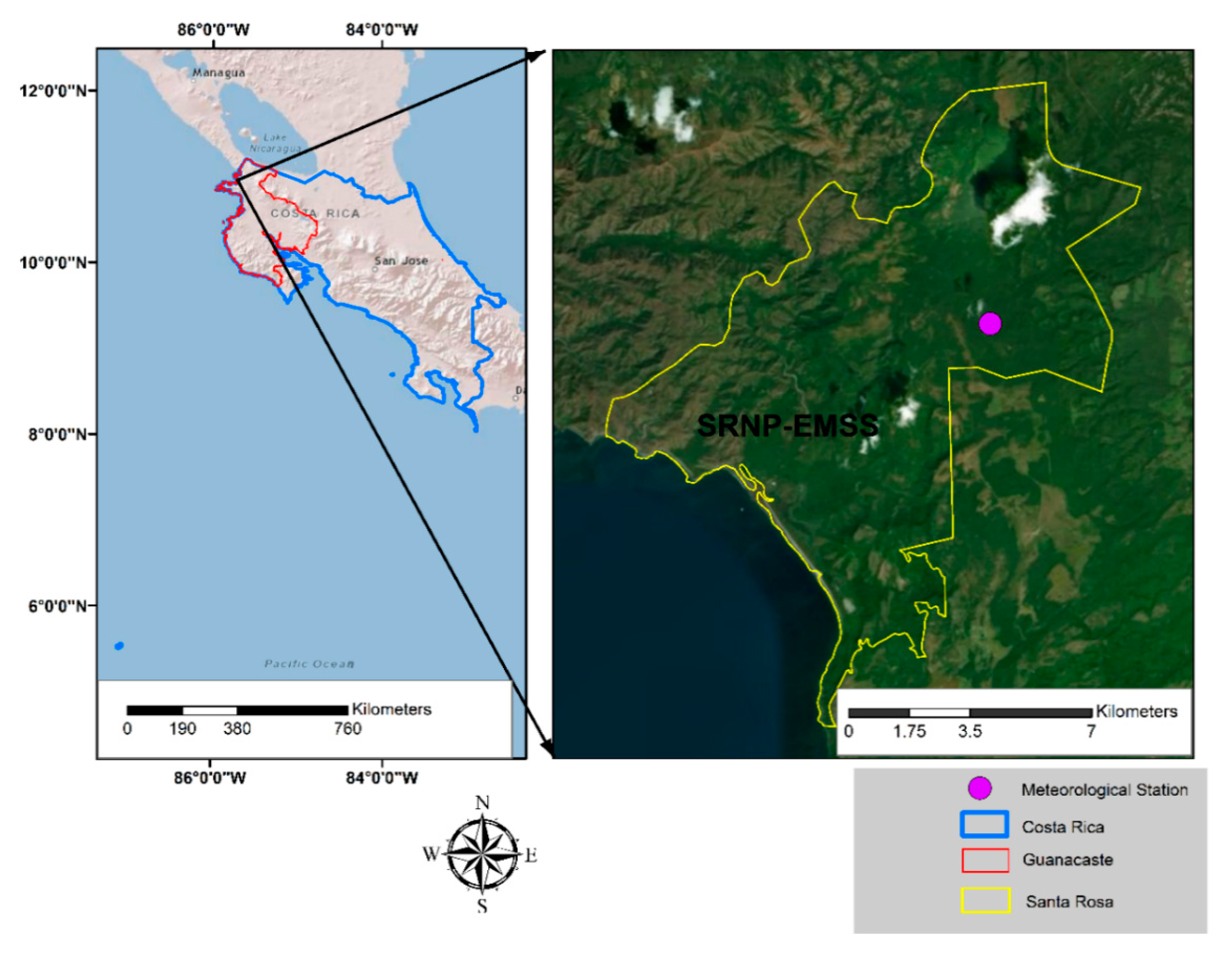
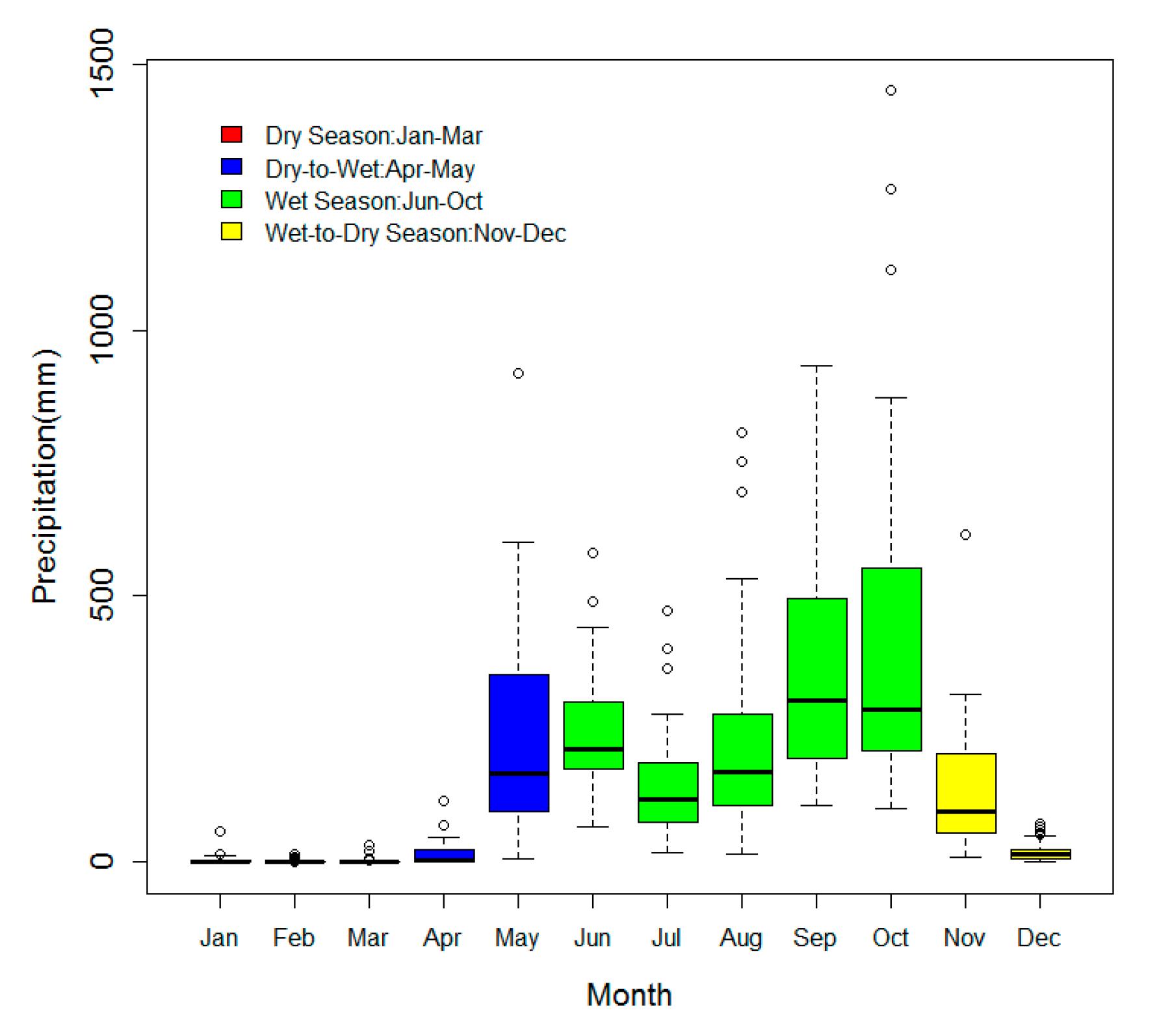
2.1. Study Site
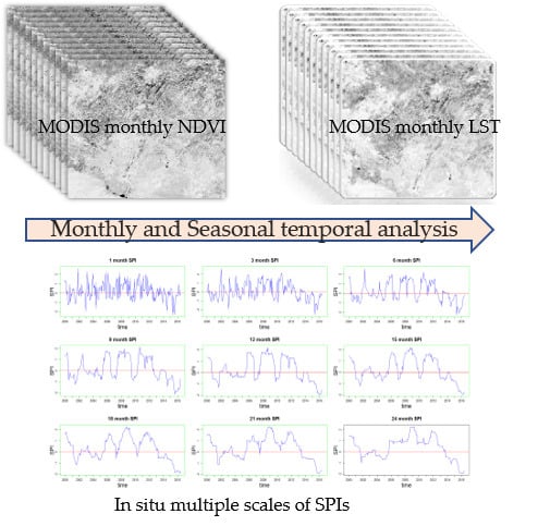
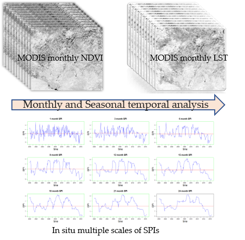
2.2. The NDVI and LST as Response Variables to Drought
2.3. Temporal Correlations Between the NDVI and LST and SPIs
2.4. The Seasonal Correlation Between the Average NDVI and LST
3. Results
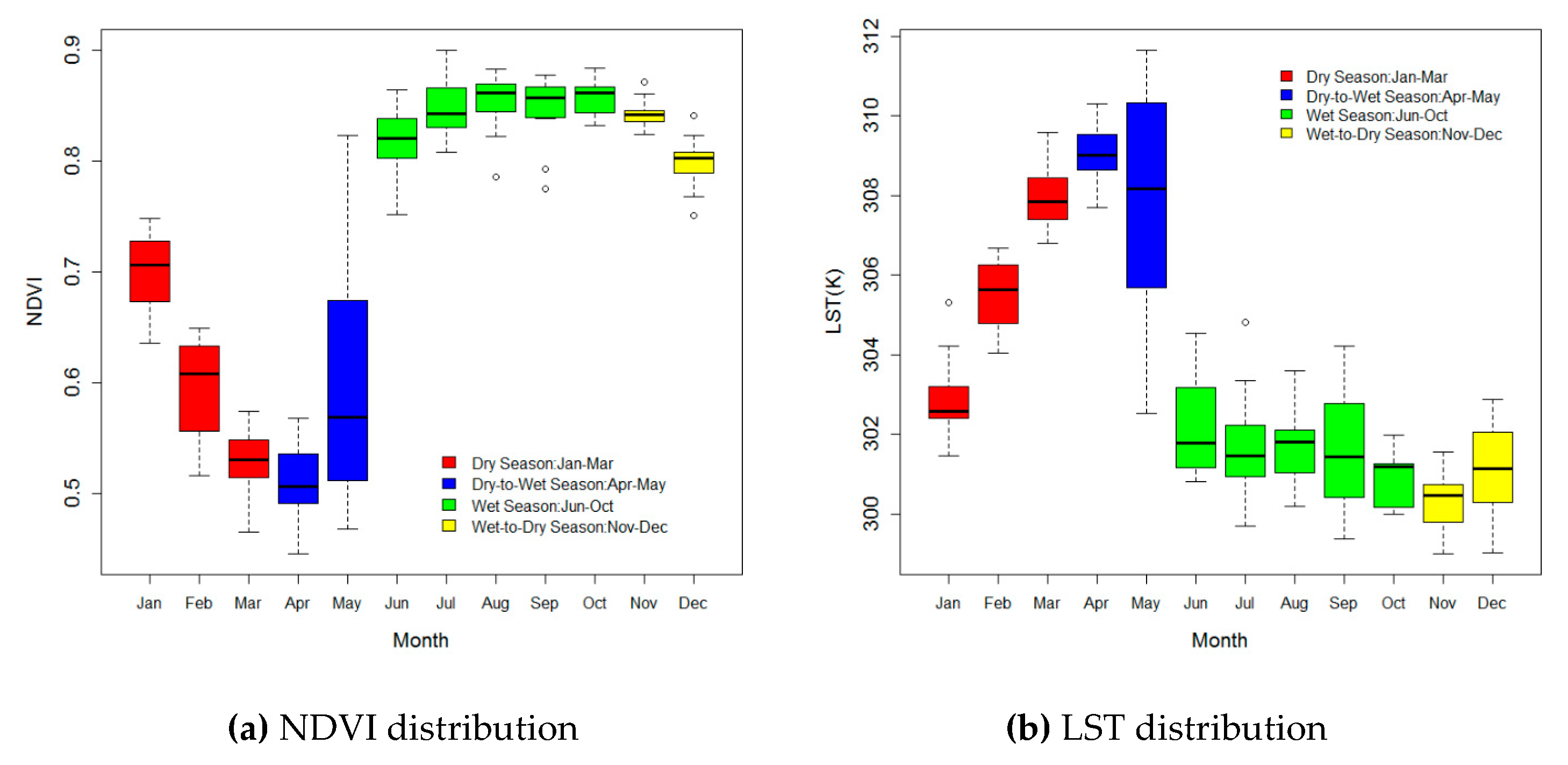
3.1. The Monthly Distribution of the NDVI and LST at SRNP-EMSS
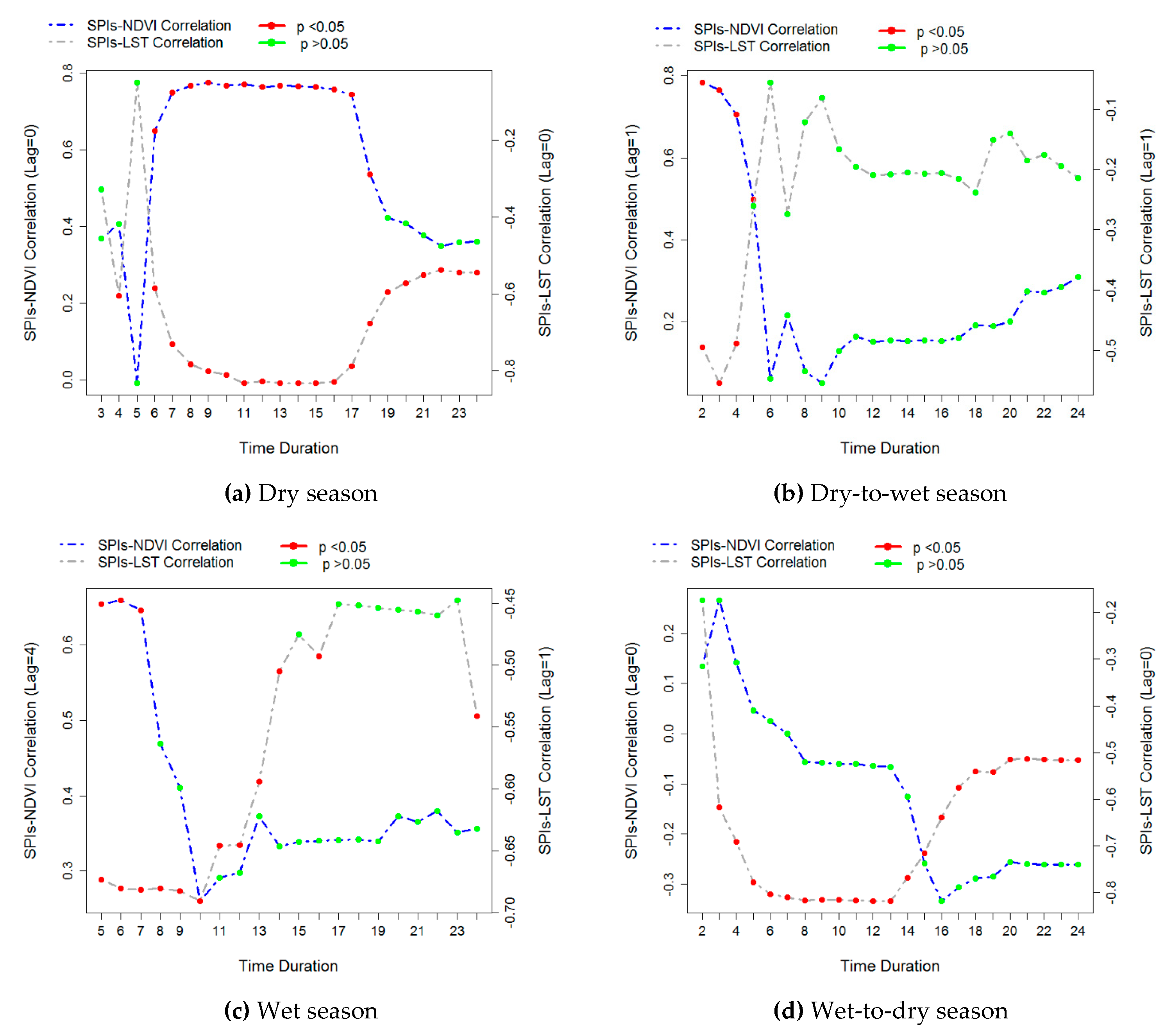
3.2. The Temporal Response of the NDVI and LST to Meteorological Drought
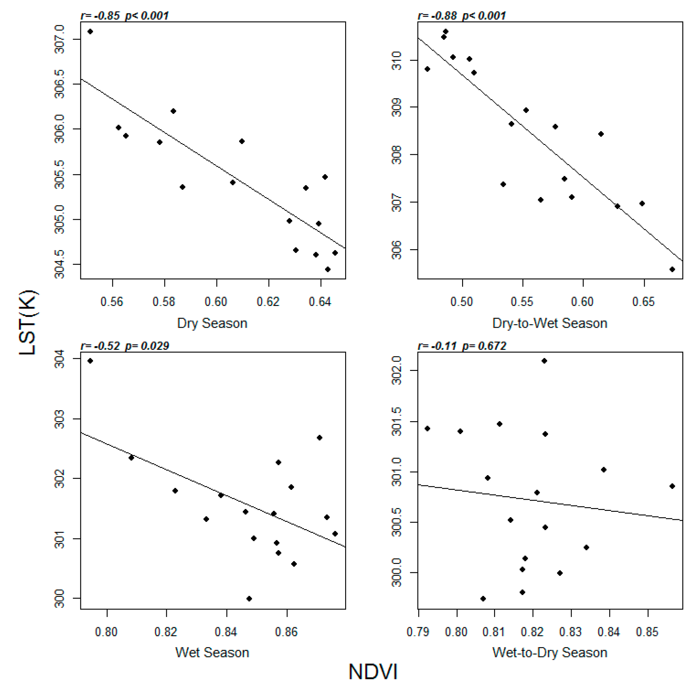
3.3. Correlation Between the Seasonal Average NDVI and LST
4. Discussion
4.1. Phenologically Dependent Responses of NDVI and LST to Meteorological Drought
4.2. Water Availability, Duration, and Timing as Key Factors Controlling the NDVI and LST
4.3. Estimate the Primary Response of TDFs to Meteorological Drought
5. Conclusions
Supplementary Materials
Author Contributions
Funding
Conflicts of Interest
References
- Sanchez-Azofeifa, G.A.; Quesada, M.; Rodríguez, J.P.; Nassar, J.M.; Stoner, K.E.; Castillo, A.; Cuevas-Reyes, P. Research priorities for Neotropical dry forests. Biotropica 2005, 37, 477–485. [Google Scholar]
- Murphy, P.G.; Lugo, A.E. Ecology of tropical dry forest. Annu. Rev. Ecol. Syst. 1986, 17, 67–88. [Google Scholar] [CrossRef]
- Quesada, M.; Sanchez-Azofeifa, G.A.; Alvarez-Anorve, M.; Stoner, K.E.; Avila-Cabadilla, L.; Calvo-Alvarado, J.; Fernandes, G.W. Succession and management of tropical dry forests in the Americas: Review and new perspectives. For. Ecol. Manag. 2009, 258, 1014–1024. [Google Scholar] [CrossRef]
- Maass, J.M.; Balvanera, P.; Castillo, A.; Daily, G.C.; Mooney, H.A.; Ehrlich, P.; García-Oliva, F. Ecosystem services of tropical dry forests: Insights from long-term ecological and social research on the Pacific Coast of Mexico. Ecol. Soc. 2005, 10, 1–23. [Google Scholar] [CrossRef]
- Balvanera, P.; Castillo, A.; Martínez-Harms, M.J. Ecosystem services in seasonally dry tropical forests. In Seasonally Dry Tropical Forests; Dirzo, R., Young, H.S., Mooney, H.A., Ceballos, G., Eds.; Island Press: Washington, DC, USA, 2011; pp. 259–277. [Google Scholar]
- Calvo-Rodriguez, S.; Sanchez-Azofeifa, A.G.; Duran, S.M.; Espirito-Santo, M.M. Assessing ecosystem services in Neotropical dry forests: A systematic review. Environ. Conserv. 2017, 44, 34–43. [Google Scholar] [CrossRef]
- Janzen, D.H. Management of habitat fragments in a tropical dry forest: Growth. Ann. Mo. Bot. Gard. 1988, 75, 105–116. [Google Scholar] [CrossRef]
- Calvo-Alvarado, J.; McLennan, B.; Sánchez-Azofeifa, A.; Garvin, T. Deforestation and forest restoration in Guanacaste, Costa Rica: Putting conservation policies in context. For. Ecol. Manag. 2009, 285, 931–940. [Google Scholar] [CrossRef]
- Portillo-Quintero, C.A.; Sanchez-Azofeifa, G.A. Extent and conservation of tropical dry forests in the Americas. Biol. Conserv. 2010, 143, 144–155. [Google Scholar] [CrossRef]
- Hoekstra, J.M.; Boucher, T.M.; Ricketts, T.H.; Roberts, C. Confronting a biome crisis: Global disparities of habitat loss and protection. Ecol. Lett. 2005, 8, 23–29. [Google Scholar] [CrossRef]
- Kalacska, M.; Sanchez-Azofeifa, G.A.; Calvo-Alvarado, J.C.; Quesada, M.; Rivard, B.; Janzen, D.H. Species composition, similarity, and diversity in three successional stages of a seasonally dry tropical forest. For. Ecol. Manag. 2004, 200, 227–247. [Google Scholar] [CrossRef]
- Chadwick, W.W.; Paduan, J.B.; Clague, D.A.; Dreyer, B.M.; Merle, S.G.; Bobbitt, A.M.; Nooner, S.L. Voluminous eruption from a zoned magma body after an increase in supply rate at Axial Seamount. Geophys. Res. Lett. 2016, 43, 12063–12070. [Google Scholar] [CrossRef]
- Castro, S.M.; Sanchez-Azofeifa, G.A.; Sato, H. Effect of drought on productivity in a Costa Rican tropical dry forest. Environ. Res. Lett. 2018, 13, 045001. [Google Scholar] [CrossRef]
- Olukayode Oladipo, E. A comparative performance analysis of three meteorological drought indices. Int. J. Climatol. 1985, 5, 655–664. [Google Scholar] [CrossRef]
- Williams, A.P.; Allen, C.D.; Macalady, A.K.; Griffin, D.; Woodhouse, C.A.; Meko, D.M.; Grissino-Mayer, H.D. Temperature as a potent driver of regional forest drought stress and tree mortality. Nat. Clim. Chang. 2013, 3, 292–297. [Google Scholar] [CrossRef]
- Patel, N.R.; Chopra, P.; Dadhwal, V.K. Analyzing spatial patterns of meteorological drought using standardized precipitation index. Meterol. Appl. 2007, 14, 329–336. [Google Scholar] [CrossRef]
- Onyutha, C. On Rigorous Drought Assessment using Daily Time Scale: Non-Stationary Frequency Analyses, Revisited Concepts, and a New Method to Yield Non-Parametric Indices. Hydrology 2017, 4, 48. [Google Scholar] [CrossRef]
- McKee, T.B.; Doeskin, N.J.; Kleist, J. The relationship of drought frequency and duration to time scales. In Proceedings of the Eighth Conference on Applied Climatology, Anaheim, CA, USA, 17–22 January 1993. [Google Scholar]
- Vicente-Serrano, S.; Beguería, S.; López-Moreno, J.I. A multiscalar drought index sensitive to global warming: The standardized precipitation evapotranspiration index. J. Clim. 2010, 23, 1696–1718. [Google Scholar] [CrossRef]
- Palmer, W.C. Meteorological Drought; Department of Commerce Weather Bureau: Washington DC, USA, 1965; p. 58.
- Zargar, A.; Sadiq, R.; Naser, B.; Khan, F.I. A review of drought indices. Environ. Rev. 2011, 19, 333–349. [Google Scholar] [CrossRef]
- Allen, C.D.; Breshears, D.D.; McDowell, N.G. On underestimation of global vulnerability to tree mortality and forest die-off from hotter drought in the Anthropocene. Ecosphere 2015, 6, 129. [Google Scholar] [CrossRef]
- Choat, B.; Jansen, S.; Brodribb, T.J.; Cochard, H.; Delzon, S.; Bhaskar, R.; Hacke, U.G. Global convergence in the vulnerability of forests to drought. Nature 2012, 491, 752–755. Available online: https://www.nature.com/articles/nature11688 (accessed on 29 November 2012). [CrossRef]
- Dale, V.H.; Joyce, L.A.; McNulty, S.; Neilson, R.P.; Ayres, M.P.; Flannigan, M.D.; Peterson, C.J. Climate change and forest disturbances: Climate change can affect forests by altering the frequency, intensity, duration, and timing of fire, drought, introduced species, insect and pathogen outbreaks, hurricanes, windstorms, ice storms, or landslides. Bioscience 2001, 51, 723–734. Available online: https://academic.oup.com/bioscience/article/51/9/723/288247 (accessed on 1 September 2001). [CrossRef]
- McDowell, N.; Pockman, W.T.; Allen, C.D.; Breshears, D.D.; Cobb, N.; Kolb, T.; Yepez, E.A. Mechanisms of plant survival and mortality during drought: Why do some plants survive while others succumb to drought? New Phytol. 2008, 178, 719–739. [Google Scholar] [CrossRef]
- Rouault, G.; Candau, J.; Lieutier, F.; Nageleisen, L.; Martin, J.; Warzée, N. Effects of drought and heat on forest insect populations in relation to the 2003 drought in Western Europe. Ann. For. Sci. 2006, 63, 613–624. [Google Scholar] [CrossRef]
- Asner, G.P.; Nepstad, D.; Cardinot, G.; Ray, D. Drought stress and carbon uptake in an Amazon forest measured with spaceborne imaging spectroscopy. Proc. Natl. Acad. Sci. USA 2004, 101, 6039–6044. [Google Scholar] [CrossRef] [PubMed]
- Anderson, L.O.; Malhi, Y.; Aragão, L.E.; Ladle, R.; Arai, E.; Barbier, N.; Phillips, O. Remote sensing detection of droughts in Amazonian forest canopies. New Phytol. 2010, 187, 733–750. [Google Scholar] [CrossRef] [PubMed]
- Lai, C.; Li, J.; Wang, Z.; Wu, X.; Zeng, X.; Chen, X.; Lian, Y.; Yu, H.; Wang, P.; Bai, X. Drought-Induced Reduction in Net Primary Productivity Across Mainland China from 1982 to 2015. Remote Sens. 2018, 10, 1433. [Google Scholar] [CrossRef]
- Phillips, O.L.; Arago, L.E.; Lewis, S.L.; Fisher, J.B.; Lloyd, J.; Lopez-Gonzalez, G.; Quesada, C.A. Drought sensitivity of the Amazon Rainforest. Science 2009, 323, 1344–1347. [Google Scholar] [CrossRef]
- Brando, P.M.; Goetz, S.J.; Baccini, A.; Nepstad, D.C.; Beck, P.S.; Christman, M.C. Seasonal and interannual variability of climate and vegetation indices across the Amazon. Proc. Natl. Acad. Sci. USA 2010, 107, 14685–14690. [Google Scholar] [CrossRef]
- Liu, J.; Sun, O.J.; Jin, H.; Zhou, Z.; Han, X. Application of two remote sensing GPP algorithms at a semiarid grassland site of north China. J. Plant Ecol. 2011, 4, 302–312. [Google Scholar] [CrossRef]
- Ji, L.; Peters, A.J. Assessing vegetation response to drought in the northern Great Plains using vegetation and drought indices. Remote Sens. Environ. 2003, 87, 85–98. [Google Scholar] [CrossRef]
- Cao, S.; Sanchez-Azofeifa, A. Modeling seasonal surface temperature variations in secondary tropical dry forests. Int. J. Appl. Earth Obs. Geoinf. 2017, 62, 122–134. [Google Scholar] [CrossRef]
- Wang, J.; Rich, P.M.; Price, K.P. Temporal responses of NDVI to precipitation and temperature in the central Great Plains, USA. Int. J. Remote Sens. 2003, 24, 2345–2364. [Google Scholar] [CrossRef]
- Nichol, J.E.; Abbas, S. Integration of remote sensing datasets for local scale assessment and prediction of drought. Sci. Total Environ. 2015, 505, 503–507. [Google Scholar] [CrossRef] [PubMed]
- Prihodko, L.; Goward, S.N. Estimation of air temperature from remotely sensed surface observations. Remote Sens. Environ. 1997, 60, 335–346. [Google Scholar] [CrossRef]
- Goward, S.N.; Xue, Y.; Czajkowski, K.P. Evaluating land surface moisture conditions from the remotely sensed temperature/vegetation index measurements: An exploration with the simplified simple biosphere model. Remote Sens. Environ. 2002, 79, 225–242. [Google Scholar] [CrossRef]
- Karnieli, A.; Bayasgalan, M.; Bayarjargal, Y.; Agam, N.; Khudulmur, S.; Tucker, C.J. Comments on the use of the vegetation health index over Mongolia. Int. J. Remote Sens. 2006, 27, 2017–2024. [Google Scholar] [CrossRef]
- Cao, S.; Sanchez-Azofeifa, G.A.; Duran, S.M.; Calvo-Rodriguez, S. Estimation of aboveground net primary productivity in secondary tropical dry forests using the Carnegie–Ames–Stanford approach (CASA) model. Environ. Res. Lett. 2016, 11, 075004. [Google Scholar] [CrossRef]
- Janzen, D.H. Costa Rica’s area de Conservacin Guanacaste: A long march to survival through non-damaging biodevelopment. Biodiversity 2000, 1, 7–20. [Google Scholar] [CrossRef]
- Campos, F.A. A synthesis of long-term environmental change in Santa Rosa, Costa Rica. In Primate Life Histories, Sex Roles, and Adaptability; Kalbitzer, U., Jack, K.M., Eds.; Springer: Cham, Switzerland, 2018; pp. 331–358. [Google Scholar]
- Karnieli, A.; Agam, N.; Pinker, R.T.; Anderson, M.; Imhoff, M.L.; Gutman, G.G.; Goldberg, A. Use of NDVI and land surface temperature for drought assessment: Merits and limitations. J. Clim. 2010, 23, 618–633. [Google Scholar] [CrossRef]
- Kogan, F.N. Application of vegetation index and brightness temperature for drought detection. Adv. Space Res. 1995, 15, 91–100. [Google Scholar] [CrossRef]
- Quiring, S.M.; Ganesh, S. Evaluating the utility of the vegetation condition index (VCI) for monitoring meteorological drought in Texas. Agric. For. Meteorol. 2010, 150, 330–339. [Google Scholar] [CrossRef]
- Rhee, J.; Im, J.; Carbone, G.J. Monitoring agricultural drought for arid and humid regions using multi-sensor remote sensing data. Remote Sens. Environ. 2010, 114, 2875–2887. [Google Scholar] [CrossRef]
- Wu, D.; Zhao, X.; Liang, S.; Zhou, T.; Huang, K.; Tang, B.; Zhao, W. Time-lag Effects of Global Vegetation Responses to Climate Change. Glob. Chang. Biol. 2015, 21, 3520–3531. [Google Scholar] [CrossRef] [PubMed]
- Zhao, J.; Xu, T.; Xiao, J.; Liu, S.; Mao, K.; Song, L.; Yao, Y.; He, X.; Feng, H. Responses of Water use Efficiency to Drought in Southwest China. Remote Sens. 2020, 12, 199. [Google Scholar] [CrossRef]
- Zhang, L.; Qiao, N.; Huang, C.; Wang, S. Monitoring Drought Effects on Vegetation Productivity using Satellite Solar-Induced Chlorophyll Fluorescence. Remote Sens. 2019, 11, 378. [Google Scholar] [CrossRef]
- Zou, L.; Cao, S.; Sanchez-Azofeifa, A. Evaluating the Utility of various Drought Indices to Monitor Meteorological Drought in Tropical Dry Forests. Int. J. Biometeorol. 2020, 64, 701–711. [Google Scholar] [CrossRef] [PubMed]
- Feng, X.; Porporato, A.; Rodriguez-Iturbe, I. Changes in rainfall seasonality in the tropics. Nat. Clim. Chang. 2013, 3, 811–815. [Google Scholar] [CrossRef]
- Xiao, X.; Zhang, Q.; Braswell, B.; Urbanski, S.; Boles, S.; Wofsy, S.; Ojima, D. Modeling gross primary production of temperate deciduous broadleaf forest using satellite images and climate data. Remote Sens. Environ. 2004, 91, 256–270. [Google Scholar] [CrossRef]
- Running, S.W.; Nemani, R.R.; Heinsch, F.A.; Zhao, M.; Reeves, M.; Hashimoto, H. A continuous satellite-derived measure of global terrestrial primary production. Bioscience 2004, 54, 547–560. [Google Scholar] [CrossRef]
- Zhu, Z.; Piao, S.; Myneni, R.; Huang, M.; Zeng, Z. Greening of the Earth and its Drivers. Nat. Clim. Chang. 2016, 6, 791–795. [Google Scholar] [CrossRef]


| Duration | ||||||||||||
|---|---|---|---|---|---|---|---|---|---|---|---|---|
| Lag | 1 | 2 | 3 | 4 | 5 | 6 | 7 | 8 | 9 | 10 | 11 | 12 |
| 0 | 0 | 0–1 | 0–2 | 0–3 | 0–4 | 0–5 | 0–6 | 0–7 | 0–8 | 0–9 | 0–10 | 0–11 |
| 1 | 1 | 1–2 | 1–3 | 1–4 | 1–5 | 1–6 | 1–7 | 1–8 | 1–9 | 1–10 | 1–11 | 1–12 |
| 2 | 2 | 2–3 | 2–4 | 2–5 | 2–6 | 2–7 | 2–8 | 2–9 | 2–10 | 2–11 | 2–12 | 2–13 |
| 3 | 3 | 3–4 | 3–5 | 3–6 | 3–7 | 3–8 | 3–9 | 3–10 | 3–11 | 3–12 | 3–13 | 3–14 |
| 4 | 4 | 4–5 | 4–6 | 4–7 | 4–8 | 4–9 | 4–10 | 4–11 | 4–12 | 4–13 | 4–14 | 4–15 |
| 5 | 5 | 5–6 | 5–7 | 5–8 | 5–9 | 5–10 | 5–11 | 5–12 | 5–13 | 5–14 | 5–15 | 5–16 |
| Period | The Maximum SPI-NDVI Correlation | The Minimum SPI-LST Correlation | ||
|---|---|---|---|---|
| Month | Time | r-Value | Time | r-Value |
| January | Duration = 5 Lag = 0 | 0.55 * | Duration = 5 Lag = 0 | −0.68 * |
| February | Duration = 10 Lag = 0 | 0.79 * | Duration = 10 Lag = 0 | −0.70 * |
| March | Duration = 12 Lag = 0 | 0.87 * | Duration = 12 Lag = 0 | −0.64 * |
| April | Duration = 12 Lag = 0 | 0.63 * | Duration = 10 Lag = 0 | −0.62 * |
| May | Duration = 2 Lag = 1 | 0.76 * | Duration = 3 Lag = 1 | −0.55 * |
| June | Duration = 11 Lag = 2 | 0.65 * | Duration = 12 Lag = 1 | −0.76 * |
| July | Duration = 2 Lag = 4 | 0.66 * | Duration = 6 Lag = 2 | −0.77 * |
| August | Duration = 3 Lag = 0 | 0.41 | Duration = 9 Lag = 0 | −0.70 * |
| September | Duration = 1 Lag = 4 | 0.81 * | Duration = 1 Lag = 4 | −0.69 * |
| October | Duration = 8 Lag = 5 | 0.34 | Duration = 1 Lag = 0 | −0.54 * |
| November | Duration = 1 Lag = 2 | −0.04 | Duration = 5 Lag = 5 | −0.42 |
| December | Duration = 3 Lag = 0 | 0.38 | Duration = 7 Lag = 0 | −0.79 * |
| Period | The Maximum SPI-NDVI Correlation | The Minimum SPI-LST Correlation | ||
|---|---|---|---|---|
| Season | Time | r-value | Time | r-value |
| Dry season | Duration = 9 Lag = 0 | 0.78 * | Duration = 11 Lag = 0 | –0.83 * |
| Dry-to-wet season | Duration = 2 Lag = 1 | 0.78 * | Duration = 3 Lag = 1 | –0.55 * |
| Wet season | Duration = 6 Lag = 4 | 0.66 * | Duration = 10 Lag = 1 | –0.69 * |
| Wet-to-dry season | Duration = 3 Lag = 0 | 0.27 | Duration = 13 Lag = 0 | –0.82 * |
© 2020 by the authors. Licensee MDPI, Basel, Switzerland. This article is an open access article distributed under the terms and conditions of the Creative Commons Attribution (CC BY) license (http://creativecommons.org/licenses/by/4.0/).
Share and Cite
Zou, L.; Cao, S.; Zhao, A.; Sanchez-Azofeifa, A. Assessing the Temporal Response of Tropical Dry Forests to Meteorological Drought. Remote Sens. 2020, 12, 2341. https://doi.org/10.3390/rs12142341
Zou L, Cao S, Zhao A, Sanchez-Azofeifa A. Assessing the Temporal Response of Tropical Dry Forests to Meteorological Drought. Remote Sensing. 2020; 12(14):2341. https://doi.org/10.3390/rs12142341
Chicago/Turabian StyleZou, Lidong, Sen Cao, Anzhou Zhao, and Arturo Sanchez-Azofeifa. 2020. "Assessing the Temporal Response of Tropical Dry Forests to Meteorological Drought" Remote Sensing 12, no. 14: 2341. https://doi.org/10.3390/rs12142341
APA StyleZou, L., Cao, S., Zhao, A., & Sanchez-Azofeifa, A. (2020). Assessing the Temporal Response of Tropical Dry Forests to Meteorological Drought. Remote Sensing, 12(14), 2341. https://doi.org/10.3390/rs12142341