PercepPan: Towards Unsupervised Pan-Sharpening Based on Perceptual Loss

Abstract

In the literature of pan-sharpening based on neural networks, high resolution multispectral images as ground-truth labels generally are unavailable. To tackle the issue, a common method is to degrade original images into a lower resolution space for supervised training under the Wald’s protocol. In this paper, we propose an unsupervised pan-sharpening framework, referred to as “perceptual pan-sharpening”. This novel method is based on auto-encoder and perceptual loss, and it does not need the degradation step for training. For performance boosting, we also suggest a novel training paradigm, called “first supervised pre-training and then unsupervised fine-tuning”, to train the unsupervised framework. Experiments on the QuickBird dataset show that the framework with different generator architectures could get comparable results with the traditional supervised counterpart, and the novel training paradigm performs better than random initialization. When generalizing to the IKONOS dataset, the unsupervised framework could still get competitive results over the supervised ones.

1. Introduction

Pan-sharpening is generally described as an image fusion problem aiming to generate a high resolution multispectral (HRMS) image based on a low resolution multispectral (LRMS) image and a panchromatic (PAN) counterpart. Classical pan-sharpening methods include component substitution [1,2,3], multi-resolution analysis [4,5], and variational optimization [6,7]. Comprehensive reviews about these methods could be found in [8,9].

With the boom of deep learning, more and more researchers use neural networks to solve the pan-sharpening problem and achieve promising results. Inspired by image super-resolution [10,11,12,13], Masi et al. [14] construct a three-layer convolutional neural network for pan-sharpening. Differently, Shao et al. [15] design a deep convolutional network with two branches, one of which is for LRMS images and another for PAN images. To make full use of domain knowledge, Yang et al. [16] integrate a special-designed structure for spectral and spatial information preservation. To improve image quality further, Liu et al. [17] use generative adversarial networks (GAN) [18] to build a pan-sharpening network, called PSGAN, in which a two-stream generator is designed to receive LRMS images and PAN images simultaneously. Different from other methods [19,20,21], (deep) neural networks-based methods could efficiently extract multi-level abstract features [22,23] for performance boosting with the standard backpropagation.

In spite of those achievements, pan-sharpening always encounters an issue in which ground-truth HRMS images usually are unavailable for neural networks training. Unlike the remote sensing image classification problem [24,25], it is impossible to get ground-truth HRMS images for pan-sharpening by manual annotation. Therefore, neural networks-based methods usually follow the Wald’s protocol [26] to take the original LRMS images as labels and degrade the original LRMS and PAN images into a lower resolution space as input. This supervised learning manner would result in a pan-sharpening network $G^{\prime }$ trained in the lower resolution space. Moreover, $G^{\prime }$ could be directly evaluated in the original resolution space. This degradation method dominates for a long time in the literature of pan-sharpening.

Is it necessary to train a pan-sharpening network in a lower resolution space based on the degradation step? In this paper, we propose an unsupervised pan-sharpening framework in which a pan-sharpening network G could be directly trained in the original resolution space. The novel method does not need the degradation step for training anymore, and leverages an auxiliary reconstructor network R instead. Figure 1 illustrates the difference between the traditional supervised perspective based on the degradation step and our unsupervised perspective.

To train the unsupervised pan-sharpening framework, we suggest a novel training paradigm, referred to as “first supervised pre-training and then unsupervised fine-tuning (SPUF)”. Generally speaking, there are three successful training paradigms for deep neural networks. The first one is “first unsupervised pre-training and then supervised fine-tuning (UPSF)”. The UPSF method [27,28] usually contains a greedy layer-wise pre-training stage and outperforms random initialization [29,30]. The second one is “end to end training (E2E)”. Thanks to the appearance of large-scale labeled datasets [31,32,33], the E2E method [34,35,36,37] becomes more and more popular. The third one is “first supervised pre-training and then supervised fine-tuning (SPSF)”. Because the SPSF method could benefit from supervised pre-training, recently, it has been applied to many tasks, such as object detection [38,39,40], semantic segmentation [41,42], super-resolution [12,43], and so on. Comprehensive experiments show that pre-training is generally helpful to downstream tasks [44,45,46]. The success of pre-training, as well as the absence of HRMS images, inspires the novel SPUF paradigm for pan-sharpening networks training.

It should be noted that this paper mainly focuses on how to train pan-sharpening networks in an unsupervised manner without the degradation step. Instead of striving for high performance, we pay particular attention to the following questions:

• How can the framework and loss be designed to train pan-sharpening model G directly?
• Could supervised pre-training offer gains in the SPUF training paradigm?
• Could the unsupervised perspective outperform its supervised counterpart?

The contributions of this paper could be summarized as follows:

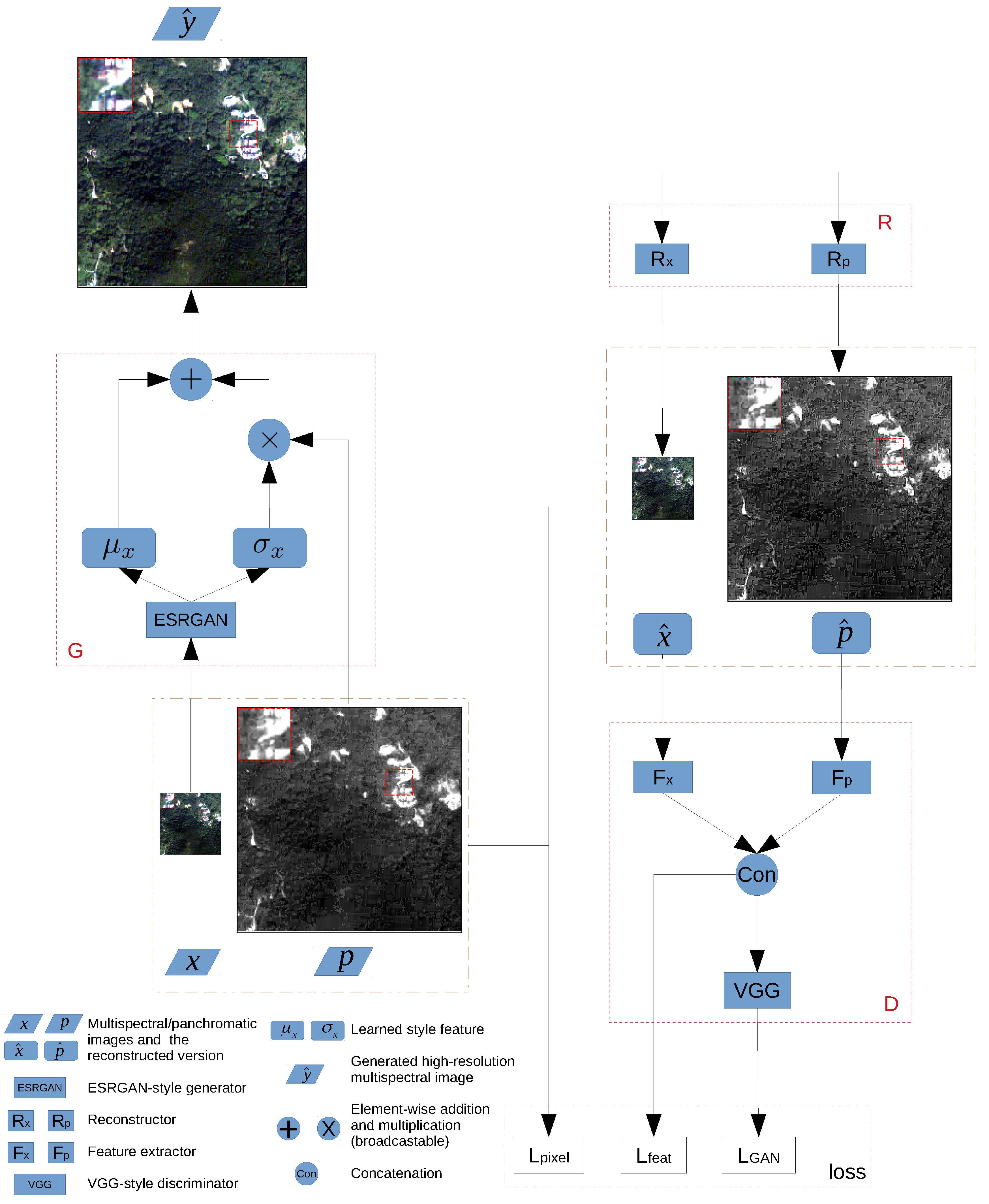
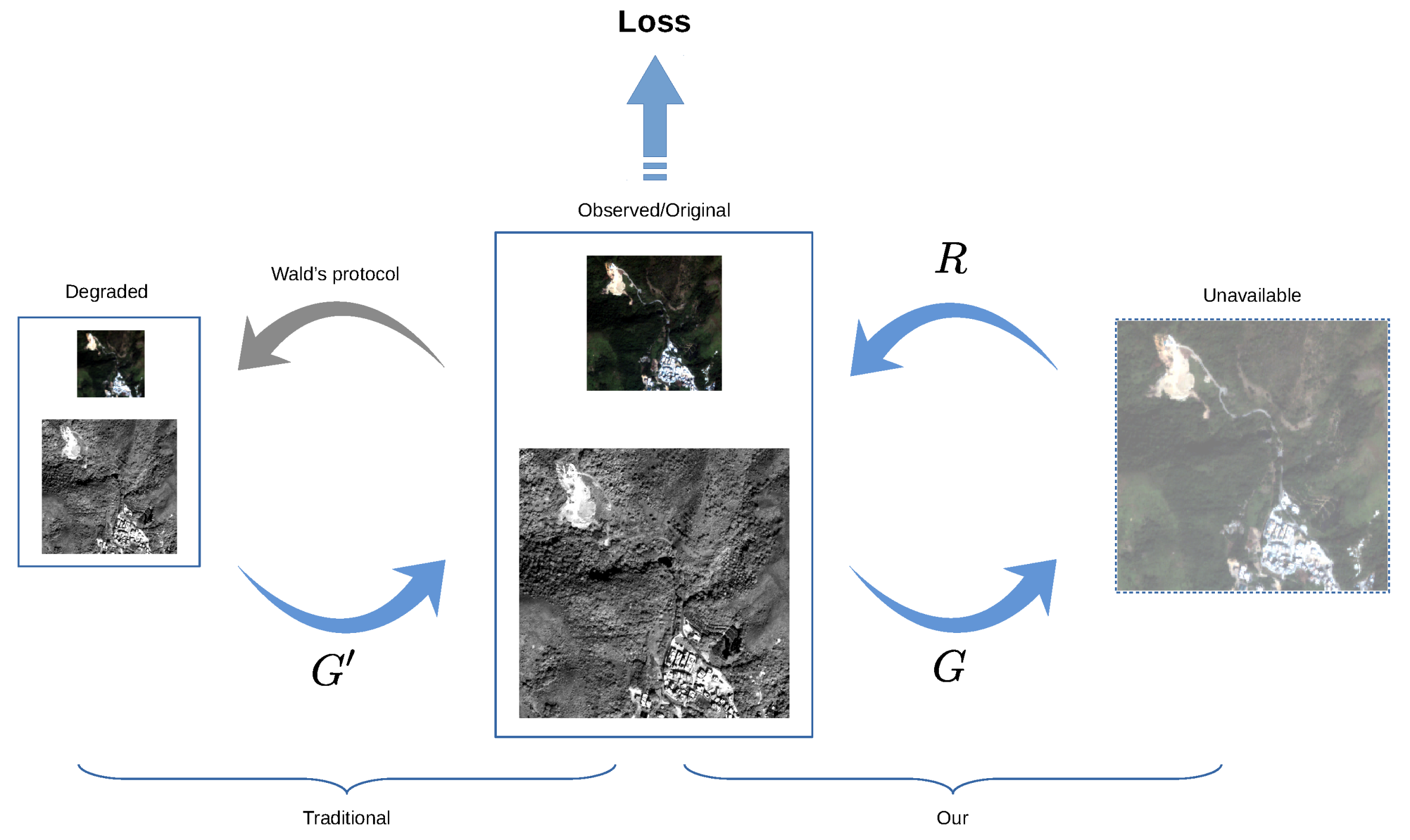
• A novel unsupervised learning framework “perceptual pan-sharpening (PercepPan)” is proposed, which does not need the degradation step anymore. The framework consists of a generator, a reconstructor, and a discriminator. The generator takes responsibility for generating HRMS images, the reconstructor takes advantage of prior knowledge to imitate the observation model from HRMS images to LRMS-PAN image pairs, and the discriminator extracts features from LRMS-PAN image pairs to compute feature loss and GAN loss.
• A perceptual loss is adopted as the objective function. The loss consists of three parts, with one computed in pixel space, another computed in feature space and the last computed in GAN space. The hybrid loss is beneficial for improving perceptual quality of generated HRMS images.
• A novel training paradigm, called SPUF, is adopted to train the proposed PercepPan. Experiments show that SPUF could usually outperform random initialization.
• Experiments show that PercepPan could cooperate with several different generators. Experiments on the QuickBird dataset show that the unsupervised results are comparable to the supervised ones. When generalizing to the IKONOS dataset, similar conclusions still hold.

The rest of this paper is organized as follows. Section 2 introduces the perceptual loss in previous works. Section 3 describes the proposed PercepPan in detail. Section 4 experimentally verifies the effectiveness of the proposed PercepPan. Finally, Section 5 concludes this paper.

2. Perceptual Loss

Basically, the proposed PercepPan is trained with perceptual loss. Perceptual loss mainly depends on high level features extracted from (convolutional) neural networks [47] rather than image pixel values. After introduced into image super-resolution [48], the loss has gotten more and more attention.

The most striking example of perceptual loss is for real-time style transfer and image super-resolution in [48], where perceptual loss is computed between real and reconstructed features by the Euclidean distance. The loss could diminish the ambiguity between high resolution images and low resolution images to some extent.

Perceptual loss could also combine with GAN loss for better performance. In the variational auto-encoder/generative adversarial network (VAE/GAN) [49], feature loss and GAN loss is combined for similarity metric learning, which could be treated as an extension of perceptual loss. It also inspires our perceptual loss for pan-sharpening. Specifically, VAE/GAN uses three different losses for training. The first one is prior loss, $\mathrm{KL}(z=\mathrm{Enc}\left(x\right)|\left|z_p\right)$, which constrains the latent representation z learned from data point x to follow the same distribution as $z_p$ drawn from a prior distribution; The second one is feature loss, $\left|\right|{\mathrm{Dis}}^{\left(l\right)}\left(x\right)-{\mathrm{Dis}}^{\left(l\right)}(\tilde{x}=\mathrm{Dec}\left(z\right)){\left|\right|}_2^2$, which is based on hidden representations from the l-th layer of the discriminator in VAE/GAN; The last one is GAN loss, $log\left(\mathrm{Dis}\left(x\right)\right)+log(1-\mathrm{Dis}\left(\tilde{x}\right))+log(1-\mathrm{Dis}\left(x_p\right))$, which could improve image sharpness. Here, $\mathrm{KL}$ means Kullback–Leibler divergence; $\mathrm{Enc}$, $\mathrm{Dec}$, and $\mathrm{Dis}$ denote the encoder, decoder, and discriminator respectively; $\tilde{x}$ and $x_p$ denote generated and reconstructed images respectively.

The proposed PercepPan adopts similar loss computation to VAE/GAN but with some differences. Specifically, PercepPan treats HRMS images as the latent representation directly, which means that the dimensionality of the representation is higher than that of the input; Moreover, PercepPan introduces loss computation in pixel space as an alternate to the prior loss.

Another example leveraging perceptual loss with GAN is enhanced super-resolution GAN (ESRGAN) [50], in which residual-in-residual dense block (RRDB) is introduced as basic unit, together with relativistic generative adversarial networks [51] and perceptual loss [48]. These tricks help ESRGAN with generating high resolution images with better perceptual quality and winning the first place in the PIRM2018-SR Challenge [52]. Mathematically, ESRGAN could be simply expressed as

$$y=\mathrm{ESRGAN}\left(x\right),$$

(1)

where x and y denote low resolution (LR) and high resolution (HR) images with three channels, respectively. Figure 2 shows the generator architecture of ESRGAN.

The proposed PercepPan also simply adopts the architecture of ESRGAN as a generator for pan-sharpening, except for minor adaptations. Specifically, images used in PercepPan are multispectral (MS) images, which usually have more channels/bands, such as four for IKONOS and QuickBird, and eight for WorldView-2, so that the number of channels of filters in the first convolutional layer needs to be changed. Moreover, PercepPan uses ESRGAN for “residual learning” rather than generating HR images directly,

$$({\mu }_x,{\sigma }_x)=\mathrm{ESRGAN}\left(x\right),$$

(2)

where x denotes a MS image, and ${\mu }_x$ and ${\sigma }_x$ are residuals, both of which have the same number of channels with x. This means that the number of channels of filters in the last convolutional layer also needs to be changed. As an example, Figure 2 also illustrates the adaptation for MS images with four bands. These learned residual would then be fused with PAN images in a manner like style transfer [53,54].

It should be noted that the proposed PercepPan could cooperate with different generators. The constructed architecture above is only an example, and it is not a crucial part of PercepPan framework.

3. Methodology

In this section, we first describe the formula of pan-sharpening as a supervised learning problem, and then present our unsupervised PercepPan framework.

3.1. Pan-Sharpening Formula

Given a training dataset with N samples, ${\left\{(x^{\left(n\right)},p^{\left(n\right)},y^{\left(n\right)})\right\}}_{n=1}^N$, where $x^{\left(n\right)}\in {\mathbb{R}}^{W\times H\times C}$, $p^{\left(n\right)}\in {\mathbb{R}}^{rW\times rH}$ and $y^{\left(n\right)}\in {\mathbb{R}}^{rW\times rH\times C}$ denote LRMS image, PAN image, and HRMS image, respectively. W, H, and C denote width, height, and the number of bands of an LRMS image respectively, and r is the spatial resolution ratio between an LRMS image and a PAN image.

When the ground-truth HRMS image $y^{\left(n\right)}$ is known, the pan-sharpening problem could be expressed as the following supervised learning problem:

$$\underset{G\in \mathcal{G}}{min}\sum _{n=1}^N\mathrm{L}({\widehat{y}}^{\left(n\right)},y^{\left(n\right)}),$$

(3)

where $\mathcal{G}$ denotes a set of pan-sharpening models/generators; $\mathrm{L}$ is a loss function, such as MSELoss (mean squared error loss) or L1Loss/MAELoss (mean absolute error loss) in pixel space; ${\widehat{y}}^{\left(n\right)}$ denotes a generated HRMS image from a pan-sharpening generator $G\in \mathcal{G}$,

$${\widehat{y}}^{\left(n\right)}=G(x^{\left(n\right)},p^{\left(n\right)}).$$

(4)

However, the ground-truth HRMS image is unavailable in fact. In this case, the loss Equation (3) could not be calculated, nor the generator G.

In this paper, we introduce auto-encoders [49,55] to deal with the absence of of HRMS images. Usually, an auto-encoder consists of an encoder learning a latent representation of an input, and a decoder (or reconstructor) reconstructing the input from the learned representation. It usually is trained by a reconstruction loss in pixel space, and does not need any labels. For pan-sharpening, the generator G plays the role of the encoder, and, in this case, the latent representation is exactly the fused HRMS image ${\widehat{y}}^{\left(n\right)}$. An extra architecture $R=(R_x,R_p)$ is introduced to reconstruct LRMS-PAN image pairs from ${\widehat{y}}^{\left(n\right)}$, and, that is to say,

$$({\widehat{x}}^{\left(n\right)},{\widehat{p}}^{\left(n\right)})=R\left({\widehat{y}}^{\left(n\right)}\right)=(R_x\left({\widehat{y}}^{\left(n\right)}\right),R_p\left({\widehat{y}}^{\left(n\right)}\right)),$$

(5)

where ${\widehat{x}}^{\left(n\right)}$ and ${\widehat{p}}^{\left(n\right)}$ denote the reconstructed LRMS and PAN images, respectively. Based on reconstructed images, loss computation could be moved from the HRMS image space to the LRMS-PAN image pair space. Hence, Equation (3) could be reformulated as

$$\underset{G\in \mathcal{G}}{min}\underset{R\in \mathcal{R}}{min}\sum _{n=1}^N\mathrm{L}({\widehat{x}}^{\left(n\right)},x^{\left(n\right)})+\mathrm{L}({\widehat{p}}^{\left(n\right)},p^{\left(n\right)}),$$

(6)

where $\mathcal{R}$ stands for a set of reconstructors.

However, computing loss only in pixel space might introduce blurring, especially when MSELoss is used [49,56]. To prevent blurring and get better perceptual quality, a hybrid loss is introduced. Generally, loss computation could be expressed as follows:

$$\mathrm{L}(M({\widehat{x}}^{\left(n\right)},{\widehat{p}}^{\left(n\right)}),M(x^{\left(n\right)},p^{\left(n\right)})),$$

(7)

in which M is an arbitrary function. When M is an identity function, it is equivalent to loss computation only in pixel space,

$$\mathrm{L}(M({\widehat{x}}^{\left(n\right)},{\widehat{p}}^{\left(n\right)}),M(x^{\left(n\right)},p^{\left(n\right)})):={\mathrm{L}}_{\mathrm{pixel}}({\widehat{x}}^{\left(n\right)},x^{\left(n\right)})+{\mathrm{L}}_{\mathrm{pixel}}({\widehat{p}}^{\left(n\right)},p^{\left(n\right)}),$$

(8)

where ${\mathrm{L}}_{\mathrm{pixel}}$ is MSELoss or L1Loss. When M is more complicated for feature extracting from LRMS-PAN image pairs, it then could be expressed as

$$\mathrm{L}(M({\widehat{x}}^{\left(n\right)},{\widehat{p}}^{\left(n\right)}),M(x^{\left(n\right)},p^{\left(n\right)})):={\mathrm{L}}_{\mathrm{feat}}(F({\widehat{x}}^{\left(n\right)},{\widehat{p}}^{\left(n\right)}),F(x^{\left(n\right)},p^{\left(n\right)})),$$

(9)

in which F is in place of M for clarity, and ${\mathrm{L}}_{\mathrm{feat}}$ is MSELoss or L1Loss. When M is a discriminator D of GAN [18], the loss could be expressed as

$$\mathrm{L}(M({\widehat{x}}^{\left(n\right)},{\widehat{p}}^{\left(n\right)}),M(x^{\left(n\right)},p^{\left(n\right)})):={\mathrm{L}}_{\mathrm{GAN}}(D({\widehat{x}}^{\left(n\right)},{\widehat{p}}^{\left(n\right)}),D(x^{\left(n\right)},p^{\left(n\right)})),$$

(10)

where ${\mathrm{L}}_{\mathrm{GAN}}$ could be BCELoss (binary cross entropy loss). These three kinds of losses could represent LRMS-PAN image pairs from different abstract levels.

Combining Equations (8)–(10) together, the optimization objective function for pan-sharpening could be expressed as follows:   

$$\underset{G\in \mathcal{G}}{min}\underset{R\in \mathcal{R}}{min}\underset{D\in \mathcal{D}}{min}\sum _{n=1}^N\alpha l_{\mathrm{pixel}}^{\left(n\right)}+\beta l_{\mathrm{feat}}^{\left(n\right)}+\gamma l_{\mathrm{GAN}}^{\left(n\right)},$$

(11)

where $\mathcal{D}$ denotes a set of discriminators,

$$\begin{array}{cc}\hfill l_{\mathrm{pixel}}^{\left(n\right)}=& {\mathrm{L}}_{\mathrm{pixel}}({\widehat{x}}^{\left(n\right)},x^{\left(n\right)})+{\mathrm{L}}_{\mathrm{pixel}}({\widehat{p}}^{\left(n\right)},p^{\left(n\right)})=\left|\right|{\widehat{x}}^{\left(n\right)}-x^{\left(n\right)}{\left|\right|}_1+\left|\right|{\widehat{p}}^{\left(n\right)}-p^{\left(n\right)}{\left|\right|}_1,\hfill \end{array}$$

(12)

$$\begin{array}{cc}\hfill l_{\mathrm{feat}}^{\left(n\right)}=& {\mathrm{L}}_{\mathrm{feat}}(F({\widehat{x}}^{\left(n\right)},{\widehat{p}}^{\left(n\right)}),F(x^{\left(n\right)},p^{\left(n\right)}))=\left|\right|F({\widehat{x}}^{\left(n\right)},{\widehat{p}}^{\left(n\right)})-F(x^{\left(n\right)},p^{\left(n\right)}){\left|\right|}_1,\hfill \end{array}$$

(13)

$$\begin{array}{cc}\hfill l_{\mathrm{GAN}}^{\left(n\right)}=& {\mathrm{L}}_{\mathrm{GAN}}(D({\widehat{x}}^{\left(n\right)},{\widehat{p}}^{\left(n\right)}),D(x^{\left(n\right)},p^{\left(n\right)}))=log(1-D({\widehat{x}}^{\left(n\right)},{\widehat{p}}^{\left(n\right)}))+log\left(D(x^{\left(n\right)},p^{\left(n\right)})\right),\hfill \end{array}$$

(14)

and $\alpha$, $\beta$ and $\gamma$ are hyper-parameters controlling the importance of different loss terms. Equation (11) could be treated as an extension of perceptual loss, which is usually used for style transfer and image super-resolution [12,48]. This is why we call the proposed model as “perceptual pan-sharpening”, or PercepPan for short. It is totally an unsupervised learning formula and does not need ground-truth HRMS images at all. It should be noticed that F is implemented as a part of D in this paper rather than an individual neural network.

Figure 3 shows the structure of our PercepPan, where G, R, and D are all implemented by neural networks. F is a part of D, and it is split into two streams, $F=(F_x,F_p)$, with $F_x$ extracting features from LRMS images and $F_p$ extracting features from PAN images. These features would be first concatenated together along channel axis and then processed by a VGG-style network [57].

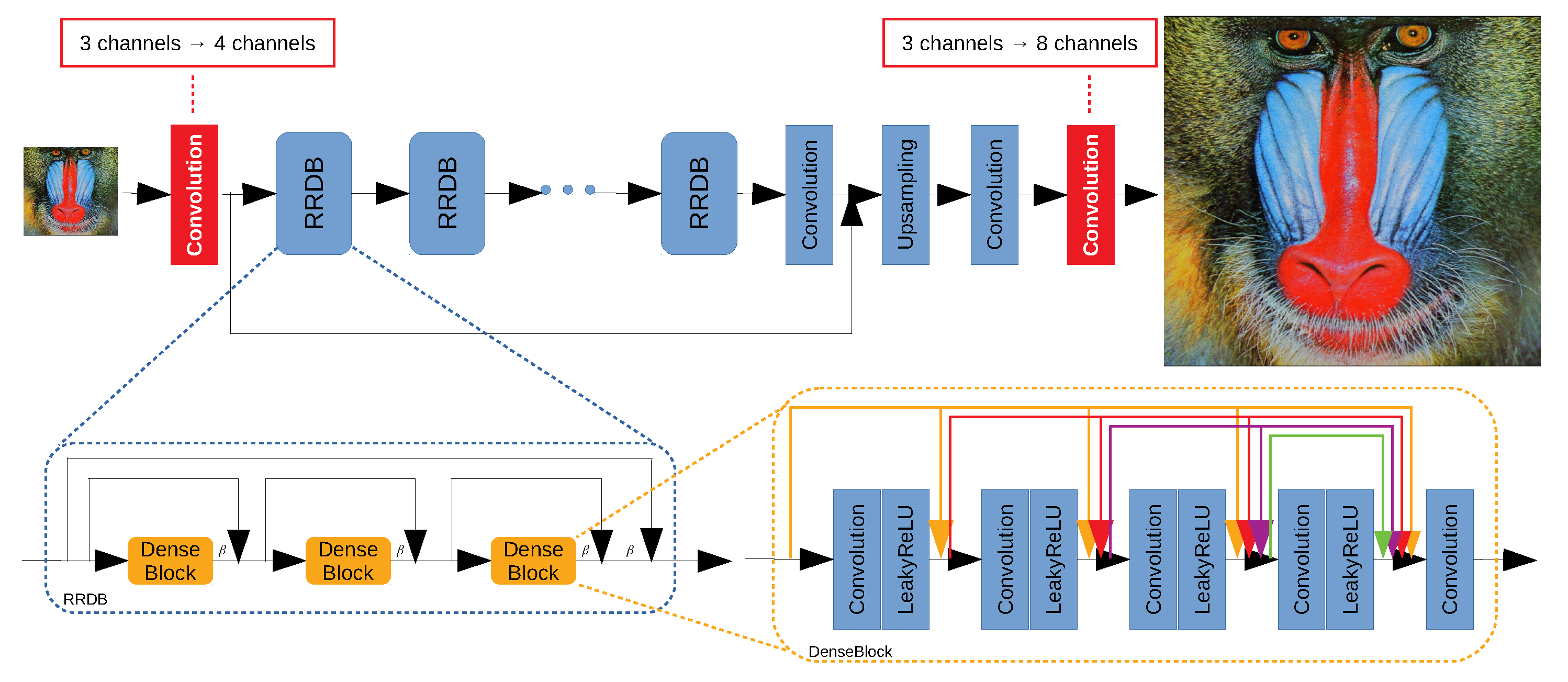
3.2. Network Architecture

As shown in Figure 3, the proposed PercepPan consists of three parts:

• A generator G which takes as input a LRMS-PAN image pair $(x,p)$ to generate a HRMS image $\widehat{y}$;
• A reconstructor R which takes as input a generated HRMS image $\widehat{y}$ to reconstruct the corresponding LRMS-PAN image pair, with the output denoted as $\widehat{x}$ and $\widehat{p}$, respectively;
• A discriminator D which takes as input real/reconstructed LRMS-PAN image pairs to calculate feature loss and GAN loss.

Generator. The generator G needs to fuse spectral details from LRMS images and spatial details from PAN images. Existing generators taking LRMS-PAN image pairs into networks directly to extract those details [14,17], or learning residual details according to LRMS images [15,16], could play the role of G. We also try the ESRGAN-style generator with residual learning according to PAN images,

$$({\widehat{y}}_1,{\widehat{y}}_2,\dots ,{\widehat{y}}_C)=({\sigma }_1,{\sigma }_2,\dots ,{\sigma }_C)\times p+({\mu }_1,{\mu }_2,\dots ,{\mu }_C),$$

(15)

where ${\widehat{y}}_c\in {\mathbb{R}}^{rH\times rW}$ is the c-th band of $\widehat{y}$, and ${\sigma }_c\in {\mathbb{R}}^{rH\times rW}$ and ${\mu }_c\in {\mathbb{R}}^{rH\times rW}$ are residuals learned from x. For simplicity, they are also denoted as ${\sigma }_x=({\sigma }_1,{\sigma }_2,\dots ,{\sigma }_C)$ and ${\mu }_x=({\mu }_1,{\mu }_2,\dots ,{\mu }_C)$, where the subscript indicates that both of them are related to x. It should be noted that multiplication and addition here are element-wise.

The residual learning is inspired by a well-known style transfer method, called “adaptive instance normalization (AdaIN)” [54]. Specifically, x is treated as style image, and the corresponding style features ${\mu }_x$ and ${\sigma }_x$ are learned by the ESRGAN-style generator, while p is treated as content image, and the content features ${\mu }_p$ and ${\sigma }_p$ are simply assigned as zero matrix and identity matrix, respectively.

Reconstructor. The reconstructor $R=(R_x,R_p)$ aims at reconstructing LRMS-PAN image pairs from the generated HRMS images. It could be implemented by a neural network. Inspired by [58], we design a shallow architecture for R to simulate the observation process about how to acquire LRMS-PAN image pairs via satellites.

Because LRMS images are spatially degraded from the corresponding HRMS images, the first part of the reconstructor, $R_x$, is treated as a combination of blurring and downsampling,

$$({\widehat{x}}_1,{\widehat{x}}_2,\dots ,{\widehat{x}}_C)=R_x({\widehat{y}}_1,{\widehat{y}}_2,\dots ,{\widehat{y}}_C):=(S\circ H_1\left({\widehat{y}}_1\right),S\circ H_2\left({\widehat{y}}_2\right),\dots ,S\circ H_C\left({\widehat{y}}_C\right)),$$

(16)

where ${\widehat{x}}_c\in {\mathbb{R}}^{W\times H}$ and ${\widehat{y}}_c\in {\mathbb{R}}^{rW\times rH}$ are the c-th spectral bands of $\widehat{x}$ and $\widehat{y}$, respectively. $H_c$ is a blurring operator for the c-th spectral band, which could be implemented as a convolutional layer, and S is a downsampling operator.

Because the PAN image generally covers all the wavelengths of the MS image spectral bands (see Section 4.1 for more detail), the PAN image could be approximated by a linear combination of the HRMS image bands [59], and, in other words, the second part of the reconstructor, $R_p$, could be defined as

$$\widehat{p}=R_p\left(\widehat{y}\right):=\sum _{c=1}^C{w}_c{\widehat{y}}_c,$$

(17)

where ${\widehat{y}}_c\in {\mathbb{R}}^{W\times H}$ is the c-th spectral band of $\widehat{y}$ and $w_c$ is the corresponding weight. The linear map could be implemented by a $1\times 1$ convolution.

Discriminator. The discriminator D is responsible for computing feature loss and GAN loss.

Feature loss computation needs LRMS-PAN image pairs as input. To receive different kinds of images simultaneously, D contains two input branches, $F=(F_x,F_p)$, with $F_x$ for LRMS images and $F_p$ for PAN images. Extracted features would then be fused together.

To compute GAN loss, D further sends these features into a VGG-style neural network [57]. For each input, the VGG-style architecture outputs a scalar, which represents the probability that the input feature is from the real data rather than the generated one.

3.3. Initialization

Initialization is crucial to training neural networks [60]. The most common strategy is random initialization according to a specific probability distribution [34,35]. Another strategy is pre-training initialization, where weights from a pre-trained network are used. The latter one has been leveraged by more and more works recently [38,50].

To initialize the generator G, both random initialization and pre-training initialization are used. For random initialization, a Gaussian distribution is used [61], denoted as Random style. For pre-training initialization, two pre-trained neural networks are used (https://github.com/xinntao/BasicSR), with one called PSNR style, which is trained with pixel loss, and the other called ESRGAN style, which is fine-tuned with GAN loss based on the former.

To initialize the reconstructor $R=(R_x,R_p)$, we develop a novel initialization strategy, called prior initialization, in which specific satellite characteristics are used. On the one hand, blurring operators $H_1,H_2,\dots ,H_C$ in $R_x$ are commonly implemented as Gaussian filters, of which weights are derived from the Nyquist cutoff frequencies of satellites [62,63]. On the other hand, the linear weights in $R_p$ could be calculated from normalized spectral response curves of satellites [58,64]. These characteristics parameters comprise the piror knowledge for initialization, and are shown in

Table 1. Nyquist cutoff frequencies (Nyquist) and linear weights (Weight) of different satellites for each spectral band.

Satellite	Item	Blue	Green	Red	Near Infrared
QuickBird	Nyquist	$0.34$	$0.32$	$0.30$	$0.22$
	Weight	$0.1139$	$0.2315$	$0.2308$	$0.4239$
IKONOS	Nyquist	$0.26$	$0.28$	$0.29$	$0.28$
	Weight	$0.1071$	$0.2646$	$0.2696$	$0.3587$

for reference. This prior knowledge plays a similar role of a regularization term, which helps to reduce the uncertainty of $\widehat{y}$.

To initialize the discriminator D, a common random initialization is enough [50], and again, a Gaussian distribution is used [61].

3.4. Training Strategy

Different parts of the proposed PercepPan need to be trained differently.

When training G, all of the losses would take effect. As Equation (11) shows, G is affected by all three kinds of losses. An individual pixel loss would result in blurring [49] while the combination of feature loss and GAN loss might introduce undesired artifacts [50]. The hybrid of three losses might diminish their drawbacks and lead to a better G.

When training D, only GAN loss would take effect. The reason is that pixel loss is computed before D so that it does not affect D at all, and feature loss would make D collapse to 0 easily in practice [49]. Therefore, D is trained by the GAN loss alone.

However, R is fixed during training. An ideal R could reflect the quality of its input faithfully by the quality of its output. When the output is terrible, the input generally is terrible as well, like the generator G. In this case, error signal is triggered only by G and the signal could help to train G properly. However, when R is terrible, it could output terrible reconstructions even if G is good enough. In this case, error signals might lead G in a wrong way. Because R is constructed and initialized by prior knowledge, it could be supposed that R is good enough and it is not necessary to train R further. Therefore, the final objective function of the proposed PercepPan for unsupervised pan-sharpening with perceptual loss is

$$\underset{G\in \mathcal{G}}{min}\underset{D\in \mathcal{D}}{min}\sum _{n=1}^N\alpha l_{\mathrm{pixel}}^{\left(n\right)}+\beta l_{\mathrm{feat}}^{\left(n\right)}+\gamma l_{\mathrm{GAN}}^{\left(n\right)}.$$

(18)

Another issue is how to balance the training procedure of G and D [65,66]. Inspired by a two time-scale update rule for training GAN [67], we use individual learning rates for G and D separately to balance the procedure. Intuitively, imagine that G and D are two learners, and error signals are knowledge that they have to learn. In general, different learners should have different learning capabilities, which could be controlled by learning rate. A great learning rate means a strong learning capability and a small one means a weak capability. In experiments, G and D would be trained with different learning rates.

3.5. Datasets and Algorithms

MS-PAN image pairs from satellites are big in size and coordinate-aligned. They usually are first cropped into small patches with proper size to construct datasets. The constructed datasets are summarized in

Table 2. Difference between full-scale and reduced-scale datasets.

Dataset	Training Paradigm	HRMS Patches	LRMS Patches	PAN Patches	Training Type	Quality Assessment
Full-scale	SPUF	None	Original MS patches	Original PAN patches	Unsupervised	No-reference
Reduced-scale	SPSF	Original MS patches	Degraded MS patches	Degraded PAN patches	Supervised	Full-reference

.

The first dataset, the full-scale dataset, is composed of these cropped patches. Compared with the original MS-PAN image pairs, these patches become smaller only in size but preserve the original spatial resolution. These patches are treated as LRMS-PAN image pairs, i.e., input to our PercepPan with the SPUF training paradigm. Models trained on this dataset are then assessed by no-reference indices. The related training algorithm is shown in Algorithm 1.

Algorithm 1 Full-scale SPUF training algorithm.

Require: Full-scale training dataset, number of training iterations $Iter$, batch size $bs$, learning rates ${\eta }_G$ and ${\eta }_D$, hyper-parameters $\alpha$, $\beta$ and $\gamma$.   1:  Initializing G, R and D   2:  for $i\leftarrow 1,2,\dots ,Iter$do   3:        Sampling a mini-batch of image pairs, ${\{x^{\left(n\right)},p^{\left(n\right)}\}}_{n=1}^{bs}$, from full-scale training dataset   4:        Computing loss $l_G={\sum }_{n=1}^{bs}\alpha l_{\mathrm{pixel}}^{\left(n\right)}+\beta l_{\mathrm{feat}}^{\left(n\right)}+\gamma l_{\mathrm{GAN}}^{\left(n\right)}$   5:        Computing Gradient $g_G={\nabla }_G{l}_G$   6:        Updating weights $w_G\leftarrow w_G-{\eta }_G·\mathrm{Adam}\left(w_G,g_G\right)$   7:        Sampling a mini-batch of image pairs, ${\{x^{\left(n\right)},p^{\left(n\right)}\}}_{n=1}^{bs}$, from full-scale training dataset   8:        Computing loss $l_D={\sum }_{n=1}^{bs}{l}_{\mathrm{GAN}}^{\left(n\right)}$   9:        Computing Gradient $g_D={\nabla }_D{l}_D$ 10:        Updating weights $w_D\leftarrow w_D-{\eta }_D·\mathrm{Adam}\left(w_D,g_D\right)$ 11:  end for

The second dataset, the reduced-scale dataset, is constructed under the Wald’s protocol [26] as tradition. The original MS-PAN image pairs are first cropped into small patches, and then are degraded by blurring and downsampling. These degraded patches are treated as LRMS-PAN image pairs, i.e., input to our PercepPan with the SPSF training paradigm. The original non-degraded MS patches would be treated as the ground-truth HRMS images, both for loss computation and full-reference image quality assessment. This training procedure is similar to the full-scale one and is shown in Algorithm 2. It should be noted that, for the SPSF training, the reconstructor R should be removed, and the discriminator should be adjusted according to HRMS images. These changes make Algorithm 2 save a little more time than Algorithm 1, with about $0.510$ s versus $0.525$ s for each iteration in our experiments.

Algorithm 2 Reduced-scale SPSF training algorithm.

Require: Reduced-scale training dataset, number of training iterations $Iter$, batch size $bs$, learning rates ${\eta }_G$ and ${\eta }_D$, hyper-parameters $\alpha$, $\beta$ and $\gamma$.   1:  Initializing G and D   2:  for $i\leftarrow 1,2,\dots ,Iter$do   3:        Sampling a mini-batch of image pairs, ${\{x^{\left(n\right)},p^{\left(n\right)}\}}_{n=1}^{bs}$, from reduced-scale training dataset   4:        Computing loss $l_G={\sum }_{n=1}^{bs}\alpha l_{\mathrm{pixel}}^{\left(n\right)}+\beta l_{\mathrm{feat}}^{\left(n\right)}+\gamma l_{\mathrm{GAN}}^{\left(n\right)}$   5:        Computing Gradient $g_G={\nabla }_G{l}_G$   6:        Updating weights $w_G\leftarrow w_G-{\eta }_G·\mathrm{Adam}\left(w_G,g_G\right)$   7:        Sampling a mini-batch of image pairs, ${\{x^{\left(n\right)},p^{\left(n\right)}\}}_{n=1}^{bs}$, from reduced-scale training dataset   8:        Computing loss $l_D={\sum }_{n=1}^{bs}{l}_{\mathrm{GAN}}^{\left(n\right)}$   9:        Computing Gradient $g_D={\nabla }_D{l}_D$ 10:        Updating weights $w_D\leftarrow w_D-{\eta }_D·\mathrm{Adam}\left(w_D,g_D\right)$ 11:  end for

4. Experiments

In this section, the proposed PercepPan with different training strategies is evaluated on different datasets. It is also compared with other deep learning methods for pan-sharpening.

4.1. Experiment Settings

Datasets. Images come from two different satellites, QuickBird and IKONOS.

Table 3. Spectral and spatial resolution of QuickBird and IKONOS.

Satellite	Wave Length (nm)					Spatial Resolution (m)
	Blue	Green	Red	Near Infrared	Panchromatic	Multispectral	Panchromatic
QuickBird	450–520	520–600	630-690	780–900	450–900	$2.8$	$0.7$
IKONOS	445–516	506–595	632–698	757–853	450–900	4	1

summarizes spectral and spatial information about these two satellites [68,69]:

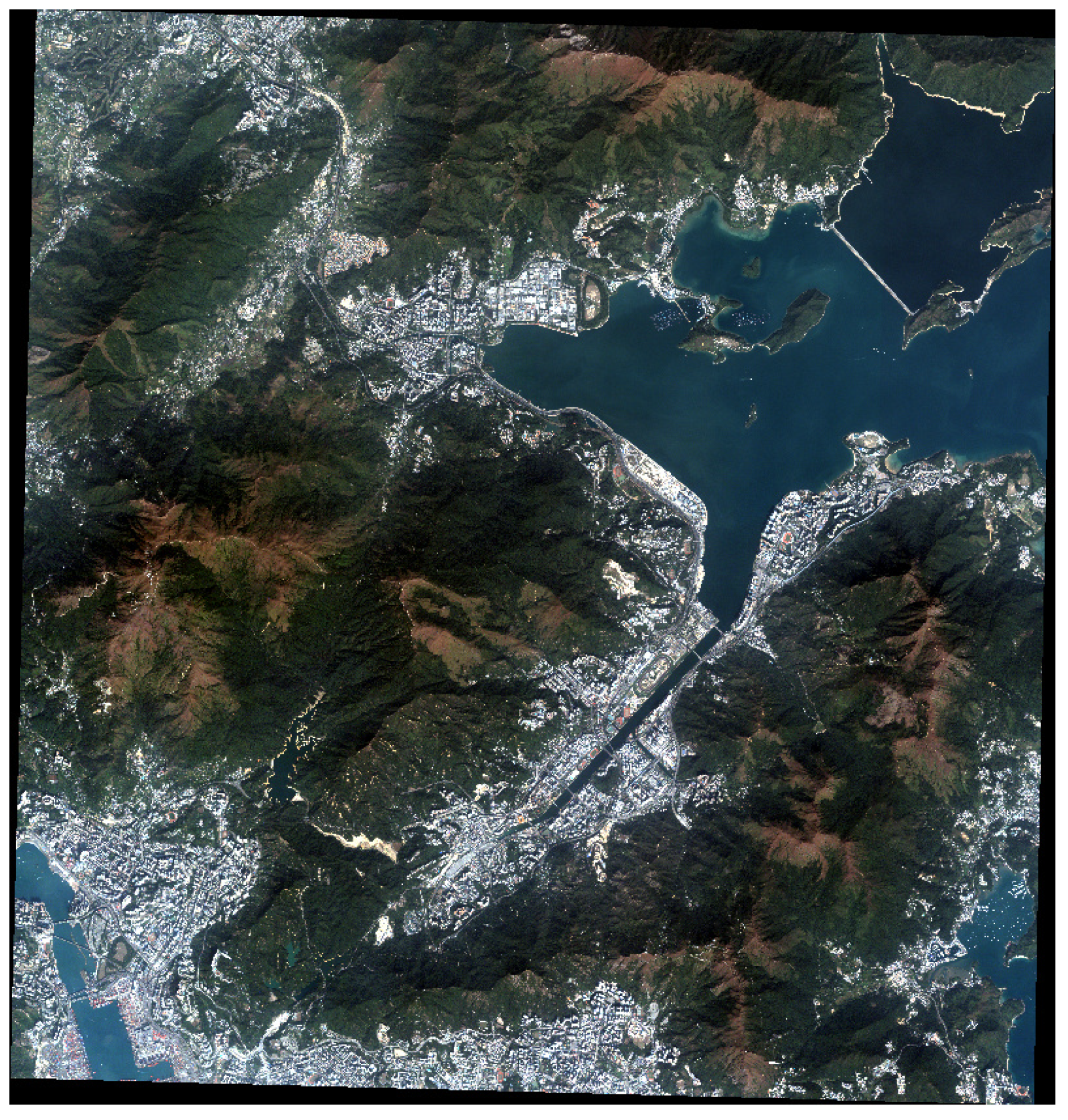
• The QuickBird bundle product is composed of two kinds of images, with one MS image at $2.8$ m resolution and another PAN images at $0.7$ m resolution, and the pixel is recorded in 11 bits. The images used in this paper come from the area of Sha Tin, Hong Kong, China, with geographic coordinates N(${22}^{°}{19}^{\prime }{58}^{″},{22}^{°}{36}^{\prime }{0}^{″}$) E(${114}^{°}{6}^{\prime }{1}^{″},{114}^{°}{16}^{\prime }{19}^{″}$), and the image of this area is shown in Figure 4. The whole size is 7364 × 7713 for MS images, and 29,456 × 30,852 for PAN images.
• The IKONOS bundle product is composed of two kinds of images as well, with one MS image at 4 m resolution and another PAN image at 1 m resolution, and again pixel is recorded in 11 bits. The images used in this paper come from the area of Wenchuan, Sichuan, China, with geographic coordinates N(${30}^{°}{59}^{\prime }{0}^{″},{31}^{°}{6}^{\prime }{0}^{″}$) E(${103}^{°}{12}^{\prime }{36}^{″},{103}^{°}{17}^{\prime }{48}^{″}$). Due to the license issue, the image of this area is not shown here. The whole size is $2066\times 3236$ for MS image, and $8264\times$ 12,944 for PAN image.

As described in Section 3.5, MS-PAN image pairs are first cropped (and/or degraded) into small patches, and then these patches are randomly split into three groups for training, validation, and test with proportion 6:2:2. Dataset information is summarized in

Table 4. Details of datasets.

Satellite	Dataset Type	Patch Size		#Training	#Validation	#Test
		Multispectral	Panchromatic
QuickBird	Full-scale	$64\times 64$	$256\times 256$	13,494	4498	4499
	Reduced-scale			820	274	274
IKONOS	Full-scale			1574	525	525
	Reduced-scale			90	30	30

. It should be noticed that the scale factor is $r=4$ in this paper, which is consistent with the rate of spatial resolution between MS and PAN images from either QuickBird or IKONOS.

Other Generators. Only neural network-based methods are used as the generator G. These methods are PNN [14], RSIFNN [15], PanNet [16], and PSGAN [17]. These methods are trained in a supervised manner with preferable settings from the corresponding papers but on our reduced-scale dataset, and then generalized onto the full-scale dataset directly. Classical methods, such as [1,4,7], are not taken into consideration.

Hyper-parameters. As stated in Section 3.3, the ESRGAN-style generator G is initialized by one of Random style, PSNR style, and ESRGAN style. The hyper-parameters in Equation (11) are given in advance, $(\alpha ,\beta ,\gamma )\in \left\{\right(1,0,0),(0,1,0.01),(1,1,0.01\left)\right\}$, in which $(1,0,0)$ means only pixel loss takes effect, $(0,1,0.01)$ means feature loss and GAN loss take effect, and $(1,1,0.01)$ means all of three losses take effect at the same time. It should be noticed that $0.01$ is used to make the GAN loss have the same order of magnitude with the other two losses in an early training stage. The batch size is assigned to be 4, and the number of iterations for training is 5000. The whole network is trained by Adam [70]. Inspired by two time scale update rule [67], learning rates ${\eta }_G$ and ${\eta }_D$ are chosen individually from 1 × 10⁻⁴ and 1 × 10⁻⁵.

All experiments are implemented on the deep learning framework, PyTorch [71] with version 4.0. All codes run on an Nvidia GTX 1080Ti GPU and an Intel Core i7 6700 CPU. The code is already available at our GitHub homepage (https://github.com/wasaCheney/PercepPan).

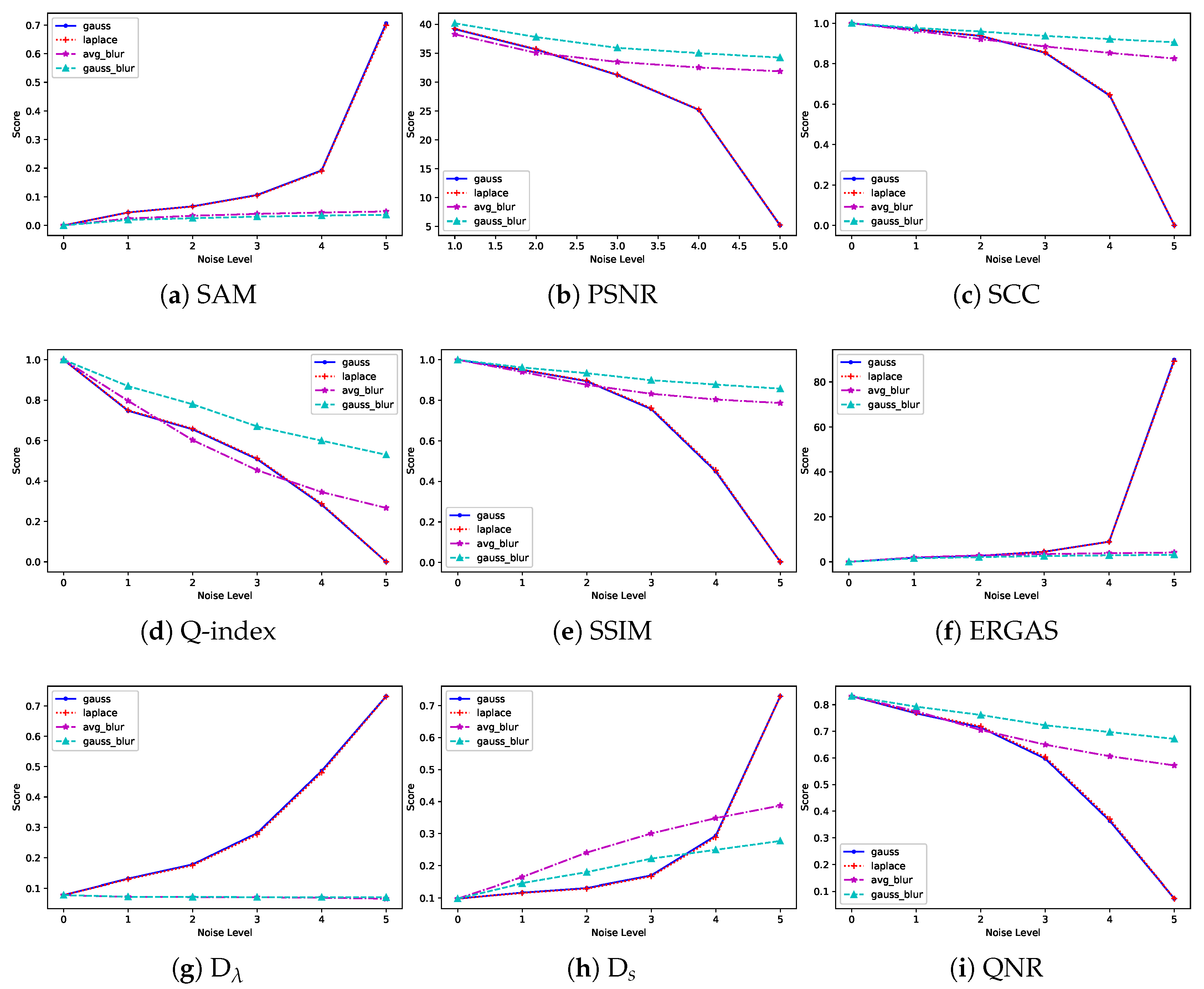
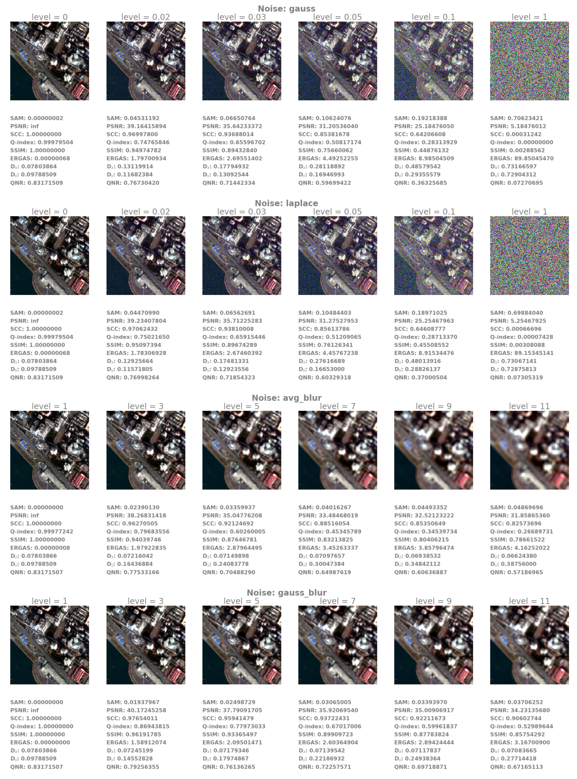
4.2. Image Quality Assessment

The proposed PercepPan together with other method is evaluated by common quality assessment indices, including full-reference indices for reduced-scale experiments, such as spectral angle mapper (SAM) [72], peak signal-to-noise ratio (PSNR), spatial correlation coefficient (SCC) [73], universal image quality index (Q-index) [74], structure similarity (SSIM) [75], and erreur relative global adimensionnelle de synthèse (ERGAS) [76]; and no-reference indices for full-scale experiments, ${\mathrm{D}}_{\lambda }$, ${\mathrm{D}}_{\mathrm{s}}$, and QNR [77]. For convenience, we simply describe them here for reference. Denote a generated image by $\widehat{I}\in {\mathbb{R}}^{H\times W\times C}$, and the corresponding ground-truth image by $I\in {\mathbb{R}}^{H\times W\times C}$, where $H,W,C$ are height, width, and number of channels, respectively.

• SAM is a measurement of spectral distortion. Denote ${\widehat{I}}_{i,j},I_{i,j}\in {\mathbb{R}}^C$ as vectors at $(i,j)$ pixel position of $\widehat{I}$ and I, respectively, then

  $$\mathrm{SAM}(\widehat{I},I)=\frac{1}{HW}\sum _{i=1}^H\sum _{j=1}^{W}arccos\frac{<{\widehat{I}}_{i,j},I_{i,j}>}{\left|\right|{\widehat{I}}_{i,j}\left|\right|\left|\right|I_{i,j}\left|\right|},$$

  where $<·,·>$ is the inner product operator.
• PSNR is a commonly used image quality assessment method,

  $$\mathrm{PSNR}(\widehat{I},I)=10{log}_{10}{\left(\frac{{\mathrm{MAX}}_I}{\mathrm{RMSE}(\widehat{I},I)}\right)}^2,$$

  (19)

  where ${\mathrm{MAX}}_I$ is the maximum possible pixel value of I, and $\mathrm{RMSE}(·,·)$ stands for the root of mean squared error. It is the same below.
• SCC is a spatial quality index. Denote ${\widehat{I}}_c,I_c\in {\mathbb{R}}^{H\times W}$ as the c-th band of $\widehat{I}$ and I, respectively. Then,

  $$\mathrm{SCC}(\widehat{I},I)=\frac{1}{C}\sum _{c=1}^C\frac{\mathrm{Cov}({\widehat{I}}_c,I_c)}{\sigma \left({\widehat{I}}_c\right)\sigma \left(I_c\right)},$$

  (20)

  where $\mathrm{Cov}(·,·)$ is the covariance and $\sigma \left(·\right)$ is the standard deviation. It is the same below.
• Q-index gathers image luminance, contrast, and structure for quality assessment. After dividing ${\widehat{I}}_c$ and $I_c$ into B patches pairs ${\left\{({\widehat{p}}_c^{\left(i\right)},p_c^{\left(i\right)})\right\}}_{i=1}^B$, Q-index is computed as follows:

  $$\mathrm{Q}(\widehat{I},I)=\frac{1}{C}\sum _{c=1}^C\frac{1}{B}\sum _{i=1}^B\frac{2\mu \left({\widehat{p}}_c^{\left(i\right)}\right)\mu \left(p_c^{\left(i\right)}\right)}{{\mu }^2\left({\widehat{p}}_c^{\left(i\right)}\right)+{\mu }^2\left(p_c^{\left(i\right)}\right)}\frac{2\sigma \left({\widehat{p}}_c^{\left(i\right)}\right)\sigma \left(p_c^{\left(i\right)}\right)}{{\sigma }^2\left({\widehat{p}}_c^{\left(i\right)}\right)+{\sigma }^2\left(p_c^{\left(i\right)}\right)}\frac{\mathrm{Cov}({\widehat{p}}_c^{\left(i\right)},p_c^{\left(i\right)})}{\sigma \left({\widehat{p}}_c^{\left(i\right)}\right)\sigma \left(p_c^{\left(i\right)}\right)},$$

  (21)

  where $\mu \left(·\right)$ stands for mean value. It is the same below.
• SSIM is a famous image quality assessment method and it is an extension of Q-index,

  $$\mathrm{SSIM}(\widehat{I},I)=\frac{1}{C}{\sum }_{c=1}^C\frac{1}{B}{\sum }_{i=1}^B\frac{2\mu \left({\widehat{p}}_c^{\left(i\right)}\right)\mu \left(p_c^{\left(i\right)}\right)+c_1}{{\mu }^2\left({\widehat{p}}_c^{\left(i\right)}\right)+{\mu }^2\left(p_c^{\left(i\right)}\right)+c_1}\frac{2\sigma \left({\widehat{p}}_c^{\left(i\right)}\right)\sigma \left(p_c^{\left(i\right)}\right)+c_2}{{\sigma }^2\left({\widehat{p}}_c^{\left(i\right)}\right)+{\sigma }^2\left(p_c^{\left(i\right)}\right)+c_2}\frac{\mathrm{Cov}({\widehat{p}}_c^{\left(i\right)},p_c^{\left(i\right)})+c_3}{\sigma \left({\widehat{p}}_c^{\left(i\right)}\right)\sigma \left(p_c^{\left(i\right)}\right)+c_3},$$

  (22)

  where $c_1={\left(0.01{\mathrm{MAX}}_I\right)}^2$, $c_2={\left(0.03{\mathrm{MAX}}_I\right)}^2$, and $c_3=MM{c}_2/2$.
• ERGAS is another common method of image quality assessment. Denote the spatial resolution ratio between MS images and the corresponding PAN images by r. Then,

  $$\mathrm{ERGAS}(\widehat{I},I)=100\times r\times \sqrt{\frac{1}{C}\sum _{c=1}^C{\left(\frac{\mathrm{RMSE}({\widehat{I}}_c,I_c)}{\mu \left(I_c\right)}\right)}^2}.$$

  (23)
• QNR is a no-reference method for image quality assessment. It consists of a spectral distortion index $D_{\lambda }$, and a spatial distortion index $D_s$. Here, denote an LRMS image with C spectral bands as $I^{\mathrm{LRMS}}$, the corresponding generated HRMS image as $I^{\mathrm{HRMS}}$, PAN image with only one spectral band as $I^{\mathrm{PAN}}$, and its degraded counterpart as $I^{\mathrm{LRPAN}}$, then

  $$\begin{array}{cc}\hfill D_{\lambda }=& {\left(\frac{2}{C(C-1)}\sum _{c=1}^C\sum _{c^{\prime }>c}^C{|Q(I_c^{\mathrm{HRMS}},I_{c^{\prime }}^{\mathrm{HRMS}})-Q(I_c^{\mathrm{LRMS}},I_{c^{\prime }}^{\mathrm{LRMS}})|}^u\right)}^{\frac{1}{u}},\hfill \end{array}$$

  (24)

  $$\begin{array}{cc}\hfill D_s=& {\left(\frac{1}{C}\sum _{c=1}^C{|Q(I_c^{\mathrm{HRMS}},I^{\mathrm{PAN}})-Q(I_c^{\mathrm{LRMS}},I^{\mathrm{LRPAN}})|}^v\right)}^{\frac{1}{v}},\hfill \end{array}$$

  (25)

  $$\begin{array}{cc}\hfill \mathrm{QNR}=& {(1-D_{\lambda })}^a{(1-D_s)}^b,\hfill \end{array}$$

  (26)

  where $u=v=1$ and $a=b=1$ usually.

Figure 5 shows the score trend of different indexes with respect to the level of noise. We choose two additive noises, Gaussian noise (gauss) and Laplace noise (laplace), which would result in spectral distortion and spatial distortion, as well as two multiplicative noises, average blur (avg_blur), and Gaussian blur (gauss_blur), which would result in spatial distortion only. As the figure shows, among full-reference indexes (the first and second rows), all of them are sensitive to the additive noises, but only Q-indexes are sensitive to the multiplicative noise; among no-reference indexes (the third row), ${\mathrm{D}}_{\lambda }$ is more sensitive to the additive noise but hardly sensitive to the multiplicative noises as its expression shows, while ${\mathrm{D}}_S$ and QNR are sensitive to both kinds of noise. Please refer to Figure A1 in Appendix A for noised images.

In summary, different indexes react differently to the level of noises, so it is necessary to assess the quality of images by combinations of different indexes. More general, assessment scores could not reflect the quality of images perfectly, so visual analysis is also necessary, especially for full-scale experiments.

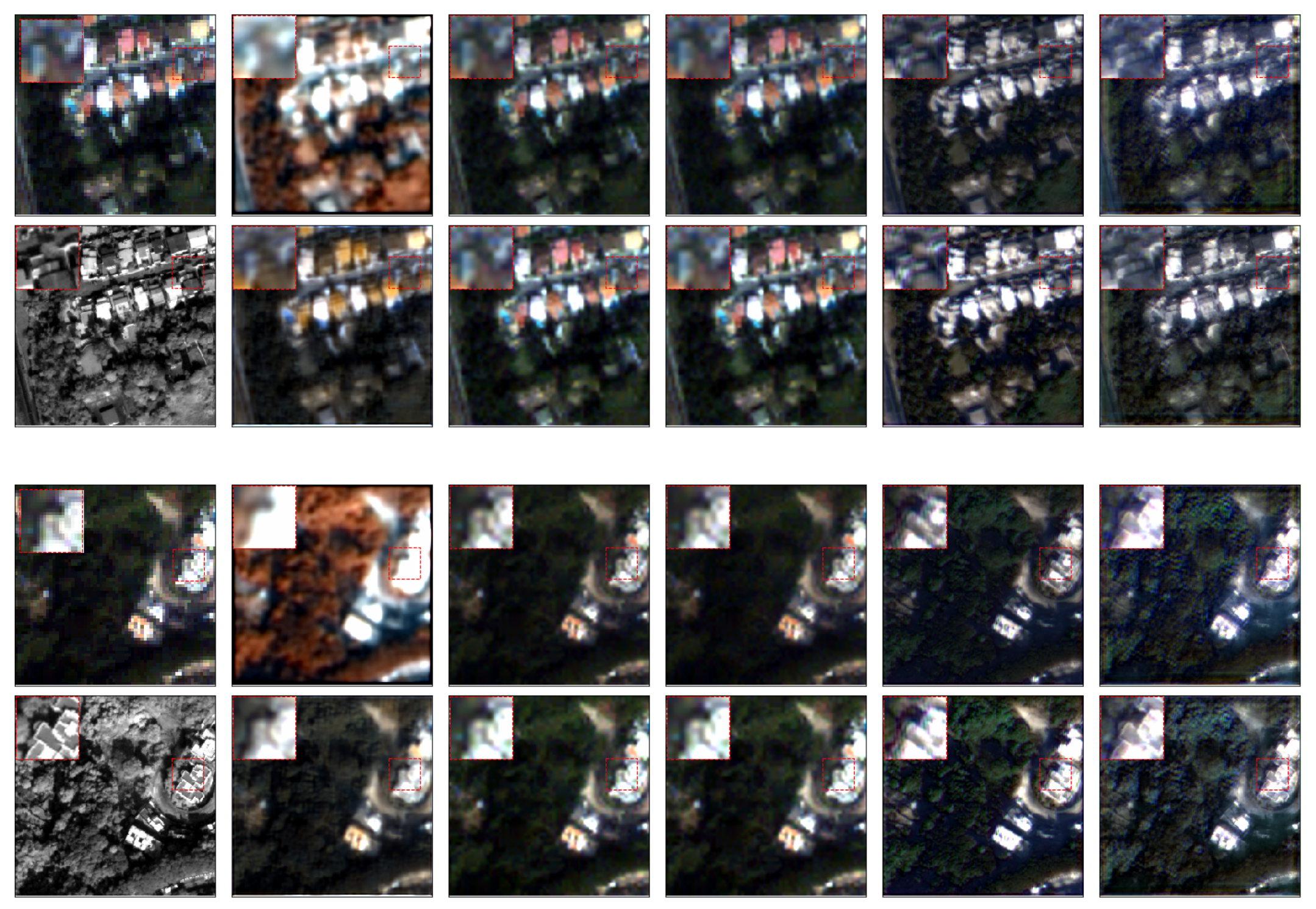
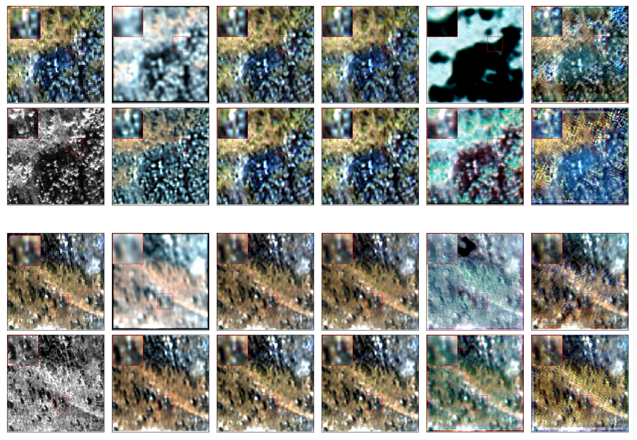
4.3. Model Evaluation with Different Settings

Table 5. Quality assessment of the proposed PercepPan under different settings on QuickBird dataset. “—” means the corresponding entry is invalid and the best value of each index is shown in parentheses.

Initialization	Hyper-Parameter					Reduced-Scale						Full-Scale
	$\mathit{\alpha }$	$\mathit{\beta }$	$\mathit{\gamma }$	${\mathit{\eta }}_{\mathit{G}}$	${\mathit{\eta }}_{\mathit{D}}$	SAM (0)	PSNR (∞)	SCC (1)	Q-index (1)	SSIM (1)	ERGAS (0)	${\mathbf{D}}_{\mathit{\lambda }}$ (0)	${\mathbf{D}}_{\mathbf{s}}$ (0)	QNR (1)
Random	1	0	0	1 × 10−4	—	$0.121$	$33.494$	$0.656$	$0.381$	$0.891$	$4.938$	$0.148/0.160$	$0.225/0.151$	$0.660/0.714$
				1 × 10−5	—	$0.125$	$33.051$	$0.631$	$0.347$	$0.871$	$5.113$	$0.136/0.151$	$0.299/0.180$	$0.605/0.697$
	0	1	$0.01$	1 × 10−4	1 × 10−4	$0.137$	$31.505$	$0.731$	$0.441$	$0.888$	$10.035$	$0.167/0.135$	$0.176/0.145$	$0.686/0.740$
				1 × 10−4	1 × 10−5	$0.118$	$35.023$	$0.745$	$\mathbf{0.495}$	$\mathbf{0.919}$	$6.641$	$0.156/0.158$	$0.164/\mathbf{0.101}$	$0.705/\mathbf{0.756}$
				1 × 10−5	1 × 10−4	$0.131$	$32.830$	$0.674$	$0.424$	$0.904$	$6.034$	$0.191/0.137$	$0.162/0.144$	$0.678/0.738$
	1	1	$0.01$	1 × 10−4	1 × 10−4	$\mathbf{0.098}$	$35.628$	$0.704$	$0.424$	$0.909$	$4.179$	$0.192/0.152$	$0.186/0.141$	$0.658/0.729$
				1 × 10−4	1 × 10−5	$0.107$	$\mathbf{35.651}$	$\mathbf{0.748}$	$0.453$	$0.912$	$\mathbf{4.009}$	$\mathbf{0.131}/\mathbf{0.118}$	$\mathbf{0.129}/0.168$	$\mathbf{0.756}/0.734$
				1 × 10−5	1 × 10−4	$0.124$	$34.128$	$0.701$	$0.425$	$0.902$	$5.197$	$0.173/0.141$	$0.174/0.153$	$0.684/0.727$
PSNR	1	0	0	1 × 10−4	—	$0.116$	$34.505$	$0.806$	$0.459$	$0.902$	$4.400$	$0.155/0.142$	$0.237/0.148$	$0.644/0.731$
				1 × 10−5	—	$0.213$	$29.682$	$0.607$	$0.371$	$0.872$	$8.544$	$0.246/0.147$	$0.262/0.129$	$0.556/0.743$
	0	1	$0.01$	1 × 10−4	1 × 10−4	$0.112$	$34.213$	$0.755$	$0.467$	$0.921$	$8.800$	$0.146/0.147$	$0.139/\mathbf{0.114}$	$0.735/0.756$
				1 × 10−4	1 × 10−5	$\mathbf{0.087}$	$\mathbf{36.491}$	$0.783$	$\mathbf{0.504}$	$0.925$	$6.471$	$0.132/0.131$	$\mathbf{0.133}/0.130$	$\mathbf{0.752}/0.756$
				1 × 10−5	1 × 10−4	$0.122$	$34.336$	$0.748$	$0.464$	$0.919$	$8.066$	$0.149/0.157$	$0.152/0.164$	$0.721/0.704$
	1	1	$0.01$	1 × 10−4	1 × 10−4	$0.109$	$35.969$	$0.765$	$0.471$	$0.917$	$4.309$	$0.170/0.131$	$0.177/0.116$	$0.683/\mathbf{0.768}$
				1 × 10−4	1 × 10−5	$0.108$	$36.080$	$\mathbf{0.814}$	$0.473$	$\mathbf{0.935}$	$4.190$	$\mathbf{0.128}/0.138$	$0.140/0.117$	$0.750/0.762$
				1 × 10−5	1 × 10−4	$0.120$	$35.444$	$0.771$	$0.461$	$0.916$	$\mathbf{4.090}$	$0.143/\mathbf{0.125}$	$0.152/0.127$	$0.727/0.764$
ESRGAN	1	0	0	1 × 10−4	—	$0.118$	$33.949$	$0.676$	$0.400$	$0.897$	$4.596$	$0.151/0.162$	$0.230/0.161$	$0.654/0.703$
				1 × 10−5	—	$0.121$	$33.036$	$0.619$	$0.328$	$0.872$	$5.084$	$\mathbf{0.123}/0.144$	$0.262/0.148$	$0.647/0.730$
	0	1	$0.01$	1 × 10−4	1 × 10−4	$0.128$	$30.959$	$0.744$	$0.452$	$0.900$	$9.092$	$0.143/0.130$	$0.143/0.127$	$0.734/0.760$
				1 × 10−4	1 × 10−5	$0.104$	$35.753$	$0.762$	$\mathbf{0.487}$	$0.922$	$6.866$	$0.174/\mathbf{0.119}$	$0.168/0.129$	$0.687/\mathbf{0.768}$
				1 × 10−5	1 × 10−4	$0.130$	$33.509$	$0.686$	$0.419$	$0.907$	$5.613$	$0.179/0.152$	$0.139/\mathbf{0.110}$	$0.707/0.754$
	1	1	$0.01$	1 × 10−4	1 × 10−4	$0.108$	$35.107$	$0.684$	$0.429$	$0.912$	$5.003$	$0.148/0.122$	$0.149/0.139$	$0.725/0.756$
				1 × 10−4	1 × 10−5	$\mathbf{0.081}$	$\mathbf{36.525}$	$\mathbf{0.761}$	$0.451$	$\mathbf{0.926}$	$\mathbf{3.479}$	$0.132/0.151$	$\mathbf{0.128}/0.111$	$\mathbf{0.757}/0.754$
				1 × 10−5	1 × 10−4	$0.117$	$34.322$	$0.656$	$0.416$	$0.915$	$4.907$	$0.186/0.123$	$0.188/0.127$	$0.660/0.766$

Notes: bold value in a column means the better combination of hyper-parameters with a specific initialization method.

shows results of the proposed PercepPan with the ESRGAN-style generator on the QuickBird dataset. In the table, “Random” means that G is initialized by a Gaussian distribution [61], “PSNR”, and “ESRGAN” mean G is initialized by pre-trained models [50]. “Reduced-scale” means networks are trained and evaluated on the reduced-scale dataset, results before “/” in “Full-scale” columns mean networks are trained on the reduced-scale dataset but evaluated on the full-scale dataset as tradition, and results after “/” in “Full-scale” columns mean networks are trained and evaluated on the full-scale dataset directly.

First of all, results on the “Reduced-scale” columns show that supervised pre-training initialization (“PSNR” and “ESRGAN” rows) generally performs better than random initialization (“Random” rows) on the pan-sharpening problem. When taking into consideration hyper-parameters $(\alpha ,\beta ,\gamma )$, in most cases, hybrid loss ($(0,1,0.01)$ and $(1,1,0.01)$ rows) performs better than pixel loss ($(1,0,0)$ rows), which suggests that hybrid loss is more suitable for pan-sharpening problem than pixel loss. As for learning rate, when only pixel loss is used, ${\eta }_G=1\times {10}^{-4}$ works better than ${\eta }_G=1\times {10}^{-5}$, but, when hybrid loss is used, $({\eta }_G,{\eta }_D)=(1\times {10}^{-4},1\times {10}^{-5})$ is more preferable.

As tradition, models trained on the reduced-scale dataset are then evaluated on the full-scale dataset (results before “/” in “Full-scale” columns). Again, pre-training initialization generally performs better than random initialization. Hybrid loss outperforms pixel loss especially on $D_s$ and QNR indices. Learning rate $({\eta }_G,{\eta }_D)=(1\times {10}^{-4},1\times {10}^{-5})$ still cooperates better with hybrid loss. All of these conclusions are consistent with those on the reduced-scale dataset.

Finally, models are trained and evaluated on the full-scale dataset (results after “/” in “Full-scale” columns). Again, similar conclusions to the above could be drawn. Moreover, when compared with traditional perspective (results before “/” in “Full-scale” columns), these unsupervised results are greater apparently. It indicates that unsupervised training directly on the full-scale dataset is more suitable for pan-sharpening.

In summary, these results suggest that pre-training initialization, hybrid loss together with $({\eta }_G,{\eta }_D)=(1\times {10}^{-4},1\times {10}^{-5})$ learning rate are preferable for the pan-sharpening problem both on the reduced-scale and full-scale datasets. Furthermore, it is better to directly train networks on the full-scale dataset.

These results indicate that the answers to our second and third questions are both positive; that is to say, pre-training could offer gains in the SPUF training paradigm and the proposed unsupervised perspective is superior to the traditional supervised perspective.

4.4. Generalization: Generator

As stated above, any neural network-based pan-sharpening generator could play the role of G in the proposed PercepPan framework.

In this part, four compared pan-sharpening models are employed as the generator G in the unsupervised framework with $(\alpha ,\beta ,\gamma )=(1,1,0.01)$ and $({\eta }_G,{\eta }_D)=(1\times {10}^{-4},1\times {10}^{-5})$. As a comparison, these models are also trained in a supervised manner with recommended settings from the corresponding papers, and all of them use random initialization.

Table 6. Quality assessment of different methods under supervised/unsupervised manner on the QuickBird dataset. The best value of each index is shown in parentheses.

Methods	Reduced-Scale						Full-Scale
	SAM (0)	PSNR (∞)	SCC (1)	Q-Index (1)	SSIM (1)	ERGAS (0)	${\mathbf{D}}_{\mathit{\lambda }}$ (0)	${\mathbf{D}}_{\mathbf{s}}$ (0)	QNR (1)
PNN [14]	$0.108$	$35.225$	$0.814$	$0.217$	$0.871$	$3.861$	$0.158/\mathbf{0.122}$	$0.183/\mathbf{0.149}$	$0.688/\mathbf{0.747}$
RSIFNN [15]	$0.081$	$37.898$	$0.835$	$0.445$	$0.913$	$6.282$	$0.081/\mathbf{0.068}$	$\mathbf{0.125}/0.129$	$0.805/\mathbf{0.812}$
PanNet [16]	$0.081$	$37.910$	$0.835$	$0.444$	$0.912$	$6.279$	$0.104/\mathbf{0.072}$	$\mathbf{0.112}/0.130$	$0.794/\mathbf{0.808}$
PSGAN [17]	$0.105$	$35.458$	$0.740$	$0.463$	$0.922$	$4.127$	$\mathbf{0.123}/0.131$	$0.112/\mathbf{0.095}$	$0.779/\mathbf{0.787}$
PercePan	$0.081$	$36.525$	$0.761$	$0.451$	$0.926$	$3.479$	$\mathbf{0.132}/0.151$	$0.128/\mathbf{0.111}$	$\mathbf{0.757}/0.754$

Notes: bold value in a "A/B" form means the better result between supervised and unsupervised methods.

shows the comparison results on the QuickBird dataset.

When trained and evaluated on the reduced-scale dataset (“Reduced-scale” columns), all of these models work as well as the PercepPan with an ESRGAN-style generator. Specifically, on indices of SAM, PSNR, and SCC, these new generators outperform the ESRGAN-style generator, while on indices of Q-index, SSIM, and ERGAS, the opposite holds.

When trained on the reduced-scale dataset but evaluated on the full-scale dataset (results before “/” in “Full-scale” columns), these models outperform the PercepPan with ESRGAN-style generator. According to the QNR index, RSIFNN, PanNet, and PSGAN are better than the best results of the PercePan with the ESRGAN-style generator, that is, $0.805$, $0.794$, and $0.779$ versus $0.757$ (with ESRGAN initialization, $(\alpha ,\beta ,\gamma )=(1,1,0.01)$ and $({\eta }_G,{\eta }_D)=(1\times {10}^{-4},1\times {10}^{-5})$ in Table 5). However, it should be noticed that this paper aims at an unsupervised perspective for pan-sharpening rather than struggling for high assessment scores under the traditional perspective.

When trained and evaluated on the full-scale dataset (results after “/” in “Full-scale” columns), these models also outperform the PercepPan with the ESRGAN-style generator. However, what is more important is that these unsupervised results are greater than the supervised ones (results before “/” in “Full-scale” columns). This means our unsupervised perspective could improve these models performance, and, that is to say, the unsupervised perspective for pan-sharpening is effective.

In summary, the proposed framework could cooperate well with different generators. Results show that the unsupervised perspective is comparable with the traditional supervised one. For perceptual intuition, Figure 6 shows the fused results of two randomly selected samples from the test set, with the top two rows corresponding to one sample and the bottom two rows to another one. For each sample, the first row shows the supervised results and the second row shows the unsupervised results. In each image, the top-left box shows the zoom-in version of a selected location for a detailed comparison. It could be seen that the perceptual quality of our unsupervised manner is better than the corresponding supervised one, especially with PNN (the second column) as the generator.

4.5. Generalization: Dataset

How about generalizing the proposed unsupervised perspective onto another dataset? In this part, we evaluate those trained models on a new dataset, the IKONOS dataset. Compared with the QuickBird dataset, the dataset has different characteristics as Table 1 and Table 3 show, and it is also much smaller as Table 4 shows.

The generalization result is shown in

Table 7. Generalization performance of the different methods on the IKONOS dataset. The best value of each index is shown in parentheses.

Methods	Reduced-Scale						Full-Scale
	SAM (0)	PSNR (∞)	SCC (1)	Q-Index (1)	SSIM (1)	ERGAS (0)	${\mathbf{D}}_{\mathit{\lambda }}$ (0)	${\mathbf{D}}_{\mathbf{s}}$ (0)	QNR (1)
PNN [14]	$0.437$	$28.804$	$0.676$	$0.223$	$0.784$	$8.939$	$0.182/\mathbf{0.112}$	$0.284/\mathbf{0.234}$	$0.585/\mathbf{0.679}$
RSIFNN [15]	$0.352$	$31.898$	$0.721$	$0.366$	$0.919$	$11.758$	$\mathbf{0.055}/0.097$	$0.192/\mathbf{0.136}$	$0.764/\mathbf{0.781}$
PanNet [16]	$0.357$	$30.969$	$0.701$	$0.326$	$0.901$	$11.088$	$\mathbf{0.096}/0.109$	$0.218/\mathbf{0.130}$	$0.708/\mathbf{0.774}$
PSGAN [17]	$0.292$	$28.065$	$0.609$	$0.455$	$0.751$	$9.813$	$\mathbf{0.146}/0.153$	$0.224/\mathbf{0.162}$	$0.663/\mathbf{0.710}$
PercepPan	$0.314$	$30.836$	$0.696$	$0.252$	$0.797$	$8.639$	$\mathbf{0.171}/0.185$	$0.202/\mathbf{0.188}$	$0.660/\mathbf{0.662}$

Notes: bold value in a "A/B" form means the better result between supervised and unsupervised methods.

. Among so many trained models of the PercepPan with ESRGAN-style generator, only the one with ESRGAN initialization, $(\alpha ,\beta ,\gamma )=(1,1,0.01)$ and $({\eta }_G,{\eta }_D)=(1\times {10}^{-4},1\times {10}^{-5})$ is used because it performs pretty well on the QuickBird dataset.

Results show that, both on the reduced-scale dataset and the full-scale dataset, all trained models work indeed but perform worse to some extent. This phenomenon might be caused by the different characteristics between the IKONOS satellite and QuickBird satellite. Moreover, it could still be observed that the proposed unsupervised perspective outperforms the traditional one when evaluated on the full-scale dataset, but the superiority is mainly caused by the spatial index $D_s$, which needs further study.

For perceptual intuition, Figure 7 shows the fused results of two randomly selected samples from the test set, with the top two rows corresponding to one sample and the bottom two rows to another one. For each sample, the first row shows the supervised results and the second row shows the unsupervised results. In each image, the top-left box shows the zoom-in version of a selected location for detailed comparison. Overall, the generalization results are worse than those on the QuickBird dataset, and the conclusion is consistent with the quantitative scores. Moreover, our unsupervised results still outperform the supervised results, especially with PNN (the second column) and PSGAN (the fifth column) as the generator.

5. Conclusions

The pan-sharpening problem always encounters an issue that high resolution multispectral images are unavailable. Traditional methods follow Wald’s protocol to degrade original images for network training in a supervised manner.

In this paper, we find that the degradation step is not necessary for network training, and propose an unsupervised pan-sharpening framework PercepPan by combining auto-encoder and perceptual loss. The novel framework could work not only on reduced-scale datasets in a traditional supervised manner, but also on full-scale datasets in an unsupervised manner. Experiments on the QuickBird dataset show that the unsupervised framework cooperates well with different pan-sharpening generators, and the unsupervised results are comparable with the supervised counterparts. When generalizing to the IKONOS dataset, the unsupervised framework is still competitive.

However, it is still far from completely unsupervised pan-sharpening. As experiments show, without pre-training initialization, the proposed PercepPan performs bad. Moreover, the reconstructor needs to be initialized according to a certain satellite, which might worsen its generalization performance. Both of these issues are worthy of further consideration.

References

1. Carper, W.; Lillesand, T.; Kiefer, R. The use of intensity-hue-saturation transformations for merging SPOT panchromatic and multispectral image data. Photogramm. Eng. Remote Sens. 1990, 56, 459–467. [Google Scholar]
2. Gillespie, A.R.; Kahle, A.B.; Walker, R.E. Color enhancement of highly correlated images. II. Channel ratio and “chromaticity” transformation techniques. Remote Sens. Environ. 1987, 22, 343–365. [Google Scholar] [CrossRef]
3. Zhang, Y.; Hong, G. An IHS and wavelet integrated approach to improve pan-sharpening visual quality of natural colour IKONOS and QuickBird images. Inf. Fusion 2005, 6, 225–234. [Google Scholar] [CrossRef]
4. Khan, M.M.; Chanussot, J.; Condat, L.; Montanvert, A. Indusion: Fusion of Multispectral and Panchromatic Images Using the Induction Scaling Technique. IEEE Geosci. Remote Sens. Lett. 2008, 5, 98–102. [Google Scholar] [CrossRef] [Green Version]
5. Otazu, X.; González-Audícana, M.; Fors, O.; Núñez, J. Introduction of sensor spectral response into image fusion methods. Application to wavelet-based methods. IEEE Trans. Geosci. Remote Sens. 2005, 43, 2376–2385. [Google Scholar] [CrossRef] [Green Version]
6. Guo, M.; Zhang, H.; Li, J.; Zhang, L.; Shen, H. An Online Coupled Dictionary Learning Approach for Remote Sensing Image Fusion. IEEE J. Sel. Top. Appl. Earth Obs. Remote Sens. 2014, 7, 1284–1294. [Google Scholar] [CrossRef]
7. Zhu, X.; Bamler, R. A Sparse Image Fusion Algorithm With Application to Pan-Sharpening. IEEE Trans. Geosci. Remote Sens. 2013, 51, 2827–2836. [Google Scholar] [CrossRef]
8. Ghassemian, H. A review of remote sensing image fusion methods. Inf. Fusion 2016, 32, 75–89. [Google Scholar] [CrossRef]
9. Meng, X.; Shen, H.; Li, H.; Zhang, L.; Fu, R. Review of the pansharpening methods for remote sensing images based on the idea of meta-analysis: Practical discussion and challenges. Inf. Fusion 2019, 46, 102–113. [Google Scholar] [CrossRef]
10. Dong, C.; Loy, C.C.; He, K.; Tang, X. Image Super-Resolution Using Deep Convolutional Networks. IEEE Trans. Pattern Anal. Mach. Intell. 2016, 38, 295–307. [Google Scholar] [CrossRef] [PubMed] [Green Version]
11. Garzelli, A. A Review of Image Fusion Algorithms Based on the Super-Resolution Paradigm. Remote Sens. 2016, 8, 797. [Google Scholar] [CrossRef] [Green Version]
12. Ledig, C.; Theis, L.; Huszar, F.; Caballero, J.; Cunningham, A.; Acosta, A.; Aitken, A.P.; Tejani, A.; Totz, J.; Wang, Z.; et al. Photo-Realistic Single Image Super-Resolution Using a Generative Adversarial Network. In Proceedings of the 2017 IEEE Conference on Computer Vision and Pattern Recognition, CVPR 2017, Honolulu, HI, USA, 21–26 July 2017; pp. 105–114. [Google Scholar] [CrossRef] [Green Version]
13. Lu, T.; Wang, J.; Zhang, Y.; Wang, Z.; Jiang, J. Satellite Image Super-Resolution via Multi-Scale Residual Deep Neural Network. Remote Sens. 2019, 11, 1588. [Google Scholar] [CrossRef] [Green Version]
14. Masi, G.; Cozzolino, D.; Verdoliva, L.; Scarpa, G. Pansharpening by Convolutional Neural Networks. Remote Sens. 2016, 8, 594. [Google Scholar] [CrossRef] [Green Version]
15. Shao, Z.; Cai, J. Remote Sensing Image Fusion With Deep Convolutional Neural Network. IEEE J. Sel. Top. Appl. Earth Obs. Remote Sens. 2018, 11, 1656–1669. [Google Scholar] [CrossRef]
16. Yang, J.; Fu, X.; Hu, Y.; Huang, Y.; Ding, X.; Paisley, J.W. PanNet: A Deep Network Architecture for Pan-Sharpening. In Proceedings of the IEEE International Conference on Computer Vision ICCV 2017, Venice, Italy, 22–29 October 2017; pp. 1753–1761. [Google Scholar] [CrossRef]
17. Liu, X.; Wang, Y.; Liu, Q. Psgan: A Generative Adversarial Network for Remote Sensing Image Pan-Sharpening. In Proceedings of the 2018 IEEE International Conference on Image Processing, ICIP 2018, Athens, Greece, 7–10 October 2018; pp. 873–877. [Google Scholar] [CrossRef] [Green Version]
18. Goodfellow, I.J.; Pouget-Abadie, J.; Mirza, M.; Xu, B.; Warde-Farley, D.; Ozair, S.; Courville, A.C.; Bengio, Y. Generative Adversarial Nets. In Proceedings of the Annual Conference on Neural Information Processing Systems 2014, Montreal, QC, Canada, 8–13 December 2014; pp. 2672–2680. [Google Scholar]
19. Hong, D.; Yokoya, N.; Chanussot, J.; Zhu, X.X. CoSpace: Common Subspace Learning from Hyperspectral-Multispectral Correspondences. IEEE Trans. Geosci. Remote Sens. 2019, 57, 4349–4359. [Google Scholar] [CrossRef] [Green Version]
20. Yao, J.; Meng, D.; Zhao, Q.; Cao, W.; Xu, Z. Nonconvex-Sparsity and Nonlocal-Smoothness-Based Blind Hyperspectral Unmixing. IEEE Trans. Image Process. 2019, 28, 2991–3006. [Google Scholar] [CrossRef]
21. Hong, D.; Yokoya, N.; Chanussot, J.; Zhu, X.X. An Augmented Linear Mixing Model to Address Spectral Variability for Hyperspectral Unmixing. IEEE Trans. Image Process. 2019, 28, 1923–1938. [Google Scholar] [CrossRef] [Green Version]
22. LeCun, Y.; Bengio, Y.; Hinton, G.E. Deep learning. Nature 2015, 521, 436–444. [Google Scholar] [CrossRef] [PubMed]
23. Hong, D.; Yokoya, N.; Xia, G.; Chanussot, J.; Zhu, X. X-ModalNet: A Semi-Supervised Deep Cross-Modal Network for Classification of Remote Sensing Data. arXiv 2020, arXiv:2006.13806. [Google Scholar]
24. Hong, D.; Yokoya, N.; Ge, N.; Chanussot, J.; Zhu, X.X. Learnable manifold alignment (LeMA): A semi-supervised cross-modality learning framework for land cover and land use classification. ISPRS J. Photogramm. Remote Sens. 2019, 147, 193–205. [Google Scholar] [CrossRef]
25. Hong, D.; Wu, X.; Ghamisi, P.; Chanussot, J.; Yokoya, N.; Zhu, X.X. Invariant attribute profiles: A spatial-frequency joint feature extractor for hyperspectral image classification. IEEE Trans. Geosci. Remote Sens. 2020, 58, 3791–3808. [Google Scholar] [CrossRef] [Green Version]
26. Wald, L.; Ranchin, T.; Mangolini, M. Fusion of satellite images of different spatial resolutions: Assessing the quality of resulting images. Photogramm. Eng. Remote Sens. 1997, 63, 691–699. [Google Scholar]
27. Hinton, G.E.; Osindero, S.; Teh, Y.W. A Fast Learning Algorithm for Deep Belief Nets. Neural Comput. 2006, 18, 1527–1554. [Google Scholar] [CrossRef]
28. Vincent, P.; Larochelle, H.; Lajoie, I.; Bengio, Y.; Manzagol, P. Stacked Denoising Autoencoders: Learning Useful Representations in a Deep Network with a Local Denoising Criterion. J. Mach. Learn. Res. 2010, 11, 3371–3408. [Google Scholar]
29. Bengio, Y.; Lamblin, P.; Popovici, D.; Larochelle, H. Greedy Layer-Wise Training of Deep Networks. In Proceedings of the Twentieth Annual Conference on Neural Information Processing Systems, Vancouver, BC, Canada, 4–7 December 2006; pp. 153–160. [Google Scholar]
30. Erhan, D.; Bengio, Y.; Courville, A.C.; Manzagol, P.; Vincent, P.; Bengio, S. Why Does Unsupervised Pre-training Help Deep Learning? J. Mach. Learn. Res. 2010, 11, 625–660. [Google Scholar]
31. Deng, J.; Dong, W.; Socher, R.; Li, L.; Li, K.; Li, F. ImageNet: A large-scale hierarchical image database. In Proceedings of the 2009 IEEE Computer Society Conference on Computer Vision and Pattern Recognition (CVPR 2009), Miami, FL, USA, 20–25 June 2009; pp. 248–255. [Google Scholar] [CrossRef] [Green Version]
32. Lin, T.; Maire, M.; Belongie, S.J.; Hays, J.; Perona, P.; Ramanan, D.; Dollár, P.; Zitnick, C.L. Microsoft COCO: Common Objects in Context. In Proceedings of the Computer Vision—ECCV 2014—13th European Conference, Zurich, Switzerland, 6–12 September 2014; pp. 740–755. [Google Scholar] [CrossRef] [Green Version]
33. Zhou, B.; Lapedriza, À.; Khosla, A.; Oliva, A.; Torralba, A. Places: A 10 Million Image Database for Scene Recognition. IEEE Trans. Pattern Anal. Mach. Intell. 2018, 40, 1452–1464. [Google Scholar] [CrossRef] [Green Version]
34. Krizhevsky, A.; Sutskever, I.; Hinton, G.E. ImageNet Classification with Deep Convolutional Neural Networks. In Proceedings of the 26th Annual Conference on Neural Information Processing Systems 2012., Lake Tahoe, NV, USA, 3–6 December 2012; pp. 1106–1114. [Google Scholar]
35. He, K.; Zhang, X.; Ren, S.; Sun, J. Deep Residual Learning for Image Recognition. In Proceedings of the 2016 IEEE Conference on Computer Vision and Pattern Recognition, CVPR 2016, Las Vegas, NV, USA, 27–30 June 2016; pp. 770–778. [Google Scholar] [CrossRef] [Green Version]
36. Huang, G.; Liu, Z.; van der Maaten, L.; Weinberger, K.Q. Densely Connected Convolutional Networks. In Proceedings of the 2017 IEEE Conference on Computer Vision and Pattern Recognition, CVPR 2017, Honolulu, HI, USA, 21–26 July 2017; pp. 2261–2269. [Google Scholar] [CrossRef] [Green Version]
37. Rasti, B.; Hong, D.; Hang, R.; Ghamisi, P.; Kang, X.; Chanussot, J.; Benediktsson, J.A. Feature Extraction for Hyperspectral Imagery: The Evolution from Shallow for Deep (Overview and Toolbox). IEEE Geosci. Remote Sens. Mag. 2020. [Google Scholar] [CrossRef]
38. Girshick, R.B.; Donahue, J.; Darrell, T.; Malik, J. Rich Feature Hierarchies for Accurate Object Detection and Semantic Segmentation. In Proceedings of the 2014 IEEE Conference on Computer Vision and Pattern Recognition, CVPR 2014, Columbus, OH, USA, 23–28 June 2014; pp. 580–587. [Google Scholar] [CrossRef] [Green Version]
39. Redmon, J.; Divvala, S.K.; Girshick, R.B.; Farhadi, A. You Only Look Once: Unified, Real-Time Object Detection. In Proceedings of the 2016 IEEE Conference on Computer Vision and Pattern Recognition, CVPR 2016, Las Vegas, NV, USA, 27–30 June 2016; pp. 779–788. [Google Scholar] [CrossRef] [Green Version]
40. Wu, X.; Hong, D.; Chanuoost, J.; Tao, R.; Wang, Y. Fourier-based Rotation- invariant Feature Boosting: An Efficient Framework for Geospatial Object Detection. IEEE Geosci. Remote Sens. Lett. 2020, 17, 302–306. [Google Scholar] [CrossRef] [Green Version]
41. Shelhamer, E.; Long, J.; Darrell, T. Fully Convolutional Networks for Semantic Segmentation. IEEE Trans. Pattern Anal. Mach. Intell. 2017, 39, 640–651. [Google Scholar] [CrossRef]
42. Chen, L.; Papandreou, G.; Kokkinos, I.; Murphy, K.; Yuille, A.L. DeepLab: Semantic Image Segmentation with Deep Convolutional Nets, Atrous Convolution, and Fully Connected CRFs. IEEE Trans. Pattern Anal. Mach. Intell. 2018, 40, 834–848. [Google Scholar] [CrossRef]
43. Gao, L.; Hong, D.; Yao, J.; Zhang, B.; Gamba, P.; Chanussot, J. Spectral Superresolution of Multispectral Imagery with Joint Sparse and Low-Rank Learning. IEEE Trans. Geosci. Remote Sens. 2020. [Google Scholar] [CrossRef]
44. He, K.; Girshick, R.B.; Dollár, P. Rethinking ImageNet Pre-training. arXiv 2018, arXiv:1811.08883. [Google Scholar]
45. Kornblith, S.; Shlens, J.; Le, Q.V. Do Better ImageNet Models Transfer Better? arXiv 2018, arXiv:1805.08974. [Google Scholar]
46. Hendrycks, D.; Lee, K.; Mazeika, M. Using Pre-Training Can Improve Model Robustness and Uncertainty. In Proceedings of the 36th International Conference on Machine Learning, ICML 2019, Long Beach, CA, USA, 9–15 June 2019; pp. 2712–2721. [Google Scholar]
47. Yosinski, J.; Clune, J.; Nguyen, A.M.; Fuchs, T.J.; Lipson, H. Understanding Neural Networks Through Deep Visualization. arXiv 2015, arXiv:1506.06579. [Google Scholar]
48. Johnson, J.; Alahi, A.; Fei-Fei, L. Perceptual Losses for Real-Time Style Transfer and Super-Resolution. In Proceedings of the Computer Vision—ECCV 2016—14th European Conference, Amsterdam, The Netherlands, 11–14 October 2016; Leibe, B., Matas, J., Sebe, N., Welling, M., Eds.; Springer: Berlin, Germany, 2016; Volume 9906, pp. 694–711. [Google Scholar] [CrossRef] [Green Version]
49. Larsen, A.B.L.; Sønderby, S.K.; Larochelle, H.; Winther, O. Autoencoding beyond pixels using a learned similarity metric. In Proceedings of the 33nd International Conference on Machine Learning, ICML 2016, New York, NY, USA, 19–24 June 2016; pp. 1558–1566. [Google Scholar]
50. Wang, X.; Yu, K.; Wu, S.; Gu, J.; Liu, Y.; Dong, C.; Qiao, Y.; Loy, C.C. ESRGAN: Enhanced Super-Resolution Generative Adversarial Networks. In Proceedings of the Computer Vision—ECCV 2018 Workshops, Munich, Germany, 8–14 September 2018; pp. 63–79. [Google Scholar] [CrossRef] [Green Version]
51. Jolicoeur-Martineau, A. The relativistic discriminator: a key element missing from standard GAN. In Proceedings of the 7th International Conference on Learning Representations, ICLR 2019, New Orleans, LA, USA, 6–9 May 2019. [Google Scholar]
52. Blau, Y.; Mechrez, R.; Timofte, R.; Michaeli, T.; Zelnik-Manor, L. The 2018 PIRM Challenge on Perceptual Image Super-Resolution. In Proceedings of the Computer Vision—ECCV 2018 Workshops, Munich, Germany, 8–14 September 2018; pp. 334–355. [Google Scholar] [CrossRef] [Green Version]
53. Ulyanov, D.; Vedaldi, A.; Lempitsky, V.S. Instance Normalization: The Missing Ingredient for Fast Stylization. arXiv 2016, arXiv:1607.08022. [Google Scholar]
54. Huang, X.; Belongie, S.J. Arbitrary Style Transfer in Real-Time with Adaptive Instance Normalization. In Proceedings of the IEEE International Conference on Computer Vision, ICCV 2017, Venice, Italy, 22–29 October 2017; pp. 1510–1519. [Google Scholar] [CrossRef] [Green Version]
55. Goodfellow, I.J.; Bengio, Y.; Courville, A.C. Deep Learning; Adaptive Computation and Machine Learning; MIT Press: Cambridge, MA, USA, 2016; pp. 499–523. [Google Scholar]
56. Isola, P.; Zhu, J.; Zhou, T.; Efros, A.A. Image-to-Image Translation with Conditional Adversarial Networks. In Proceedings of the 2017 IEEE Conference on Computer Vision and Pattern Recognition, CVPR 2017, Honolulu, HI, USA, 21–26 July 2017; pp. 5967–5976. [Google Scholar] [CrossRef] [Green Version]
57. Simonyan, K.; Zisserman, A. Very Deep Convolutional Networks for Large-Scale Image Recognition. In Proceedings of the 3rd International Conference on Learning Representations, ICLR 2015, San Diego, CA, USA, 7–9 May 2015. [Google Scholar]
58. Li, S.; Yin, H.; Fang, L. Remote Sensing Image Fusion via Sparse Representations Over Learned Dictionaries. IEEE Trans. Geosci. Remote Sens. 2013, 51, 4779–4789. [Google Scholar] [CrossRef]
59. Hong, D.; Zhu, X. SULoRA: Subspace Unmixing with Low-Rank Attribute Embedding for Hyperspectral Data Analysis. IEEE J. Sel. Top. Signal Process. 2018, 12, 1351–1363. [Google Scholar] [CrossRef]
60. Mishkin, D.; Matas, J. All you need is a good init. In Proceedings of the 4th International Conference on Learning Representations, ICLR 2016, San Juan, Puerto Rico, 2–4 May 2016. [Google Scholar]
61. He, K.; Zhang, X.; Ren, S.; Sun, J. Delving Deep into Rectifiers: Surpassing Human-Level Performance on ImageNet Classification. In Proceedings of the 2015 IEEE International Conference on Computer Vision, ICCV 2015, Santiago, Chile, 7–13 December 2015; pp. 1026–1034. [Google Scholar] [CrossRef] [Green Version]
62. Aiazzi, B.; Alparone, L.; Baronti, S.; Garzelli, A.; Selva, M. MTF-tailored multiscale fusion of high-resolution MS and Pan imagery. Photogramm. Eng. Remote Sens. 2006, 72, 591–596. [Google Scholar] [CrossRef]
63. Vivone, G.; Alparone, L.; Chanussot, J.; Mura, M.D.; Garzelli, A.; Licciardi, G.; Restaino, R.; Wald, L. A Critical Comparison Among Pansharpening Algorithms. IEEE Trans. Geosci. Remote Sens. 2015, 53, 2565–2586. [Google Scholar] [CrossRef]
64. Li, Z.; Leung, H. Fusion of Multispectral and Panchromatic Images Using a Restoration-Based Method. IEEE Trans. Geosci. Remote Sens. 2009, 47, 1482–1491. [Google Scholar] [CrossRef]
65. Radford, A.; Metz, L.; Chintala, S. Unsupervised Representation Learning with Deep Convolutional Generative Adversarial Networks. In Proceedings of the 4th International Conference on Learning Representations, ICLR 2016, San Juan, Puerto Rico, 2–4 May 2016. [Google Scholar]
66. Salimans, T.; Goodfellow, I.J.; Zaremba, W.; Cheung, V.; Radford, A.; Chen, X. Improved Techniques for Training GANs. In Proceedings of the Annual Conference on Neural Information Processing Systems 2016, Barcelona, Spain, 5–10 December 2016; pp. 2226–2234. [Google Scholar]
67. Heusel, M.; Ramsauer, H.; Unterthiner, T.; Nessler, B.; Hochreiter, S. GANs Trained by a Two Time-Scale Update Rule Converge to a Local Nash Equilibrium. In Proceedings of the Annual Conference on Neural Information Processing Systems 2017, Long Beach, CA, USA, 4–9 December 2017; pp. 6626–6637. [Google Scholar]
68. Wang, L.; Sousa, W.P.; Gong, P.; Biging, G.S. Comparison of IKONOS and QuickBird images for mapping mangrove species on the Caribbean coast of Panama. Remote Sens. Environ. 2004, 91, 432–440. [Google Scholar] [CrossRef]
69. Parente, C.; Santamaria, R. Increasing geometric resolution of data supplied by quickbird multispectral sensors. Sens. Transducers 2013, 156, 111. [Google Scholar]
70. Kingma, D.P.; Ba, J. Adam: A Method for Stochastic Optimization. In Proceedings of the 3rd International Conference on Learning Representations, ICLR 2015, San Diego, CA, USA, 7–9 May 2015. [Google Scholar]
71. Paszke, A.; Gross, S.; Massa, F.; Lerer, A.; Bradbury, J.; Chanan, G.; Killeen, T.; Lin, Z.; Gimelshein, N.; Antiga, L.; et al. PyTorch: An Imperative Style, High-Performance Deep Learning Library. In Proceedings of the Annual Conference on Neural Information Processing Systems 2019, NeurIPS 2019, Vancouver, BC, Canada, 8–14 December 2019; Wallach, H.M., Larochelle, H., Beygelzimer, A., d’Alché-Buc, F., Fox, E.B., Garnett, R., Eds.; pp. 8024–8035. [Google Scholar]
72. Yuhas, R.H.; Goetz, A.F.; Boardman, J.W. Discrimination among semi-arid landscape endmembers using the spectral angle mapper (SAM) algorithm. In Proceedings of the Summaries 3rd Annual JPL Airborne Geoscience Workshop, 1992, Pasadena, CA, USA, 1–5 June 1992; Jet Propulsion Laboratory Publication: Pasadena, CA, USA, 1992; Volume 1, pp. 147–149. [Google Scholar]
73. Zhou, J.; Civco, D.; Silander, J. A wavelet transform method to merge Landsat TM and SPOT panchromatic data. Int. J. Remote Sens. 1998, 19, 743–757. [Google Scholar] [CrossRef]
74. Wang, Z.; Bovik, A.C. A universal image quality index. IEEE Signal Process. Lett. 2002, 9, 81–84. [Google Scholar] [CrossRef]
75. Wang, Z.; Bovik, A.C.; Sheikh, H.R.; Simoncelli, E.P. Image quality assessment: from error visibility to structural similarity. IEEE Trans. Image Process. 2004, 13, 600–612. [Google Scholar] [CrossRef] [Green Version]
76. Ranchin, T.; Wald, L. Fusion of high spatial and spectral resolution images: the ARSIS concept and its implementation. Photogramm. Eng. Remote Sens. 2000, 66, 49–61. [Google Scholar]
77. Alparone, L.; Aiazzi, B.; Baronti, S.; Garzelli, A.; Nencini, F.; Selva, M. Multispectral and panchromatic data fusion assessment without reference. Photogramm. Eng. Remote Sens. 2008, 74, 193–200. [Google Scholar] [CrossRef] [Green Version]
Figure 1. Different perspectives to train pan-sharpening models. Left: traditional supervised perspective; Right: proposed unsupervised perspective.
Remotesensing 12 02318 g001
Figure 2. The generator of ESRGAN. Contents in red boxes shows an example of adaptations when taking as input MS image with four bands.
Remotesensing 12 02318 g002
Figure 3. The structure of the proposed PercepPan. G, R, and D denote Generator, Reconstructor, and Discriminator, respectively.
Remotesensing 12 02318 g003
Figure 4. Territorial framework of the investigated area from a QuickBird satellite.
Remotesensing 12 02318 g004
Figure 5. The score trend of different indexes with respect to the level of noise. On the x-axis, a greater number means a higher noise level.
Remotesensing 12 02318 g005
Figure 6. Fused results of two randomly selected samples from the QuickBird test set. From left to right are the original LRMS/PAN images, results of PNN, RSIFNN, PanNet, PSGAN, and PercepPan with the ESRGAN generator, respectively.
Remotesensing 12 02318 g006
Figure 7. Fused results of two randomly selected samples from the IKONOS test set. From left to right are the original LRMS/PAN images, results of PNN, RSIFNN, PanNet, PSGAN, and the PercepPan with the ESRGAN generator, respectively.
Remotesensing 12 02318 g007