Article

Super Resolution by Deep Learning Improves Boulder Detection in Side Scan Sonar Backscatter Mosaics

Leibniz Institute for Baltic Sea Research Warnemünde, Seestrasse 15, 18119 Warnemünde, Germany
Remote Sens. 2020, 12(14), 2284; https://doi.org/10.3390/rs12142284
Submission received: 5 June 2020 / Revised: 3 July 2020 / Accepted: 14 July 2020 / Published: 16 July 2020

Abstract

:
In marine habitat mapping, a demand exists for high-resolution maps of the seafloor both for marine spatial planning and research. One topic of interest is the detection of boulders in side scan sonar backscatter mosaics of continental shelf seas. Boulders are oftentimes numerous, but encompass few pixels in backscatter mosaics. Therefore, both their automatic and manual detection is difficult. In this study, located in the German Baltic Sea, the use of super resolution by deep learning to improve the manual and automatic detection of boulders in backscatter mosaics is explored. It is found that upscaling of mosaics by a factor of 2 to 0.25 m or 0.125 m resolution increases the performance of small boulder detection and boulder density grids. Upscaling mosaics with 1.0 m pixel resolution by a factor of 4 improved performance, but the results are not sufficient for practical application. It is suggested that mosaics of 0.5 m resolution can be used to create boulder density grids in the Baltic Sea in line with current standards following upscaling.

Graphical Abstract

1. Introduction

The need for improving the resolution of images is widespread, including tasks in medical applications, object detection, or remote sensing [1]. In marine habitat mapping by acoustic remote sensing specifically, a recent topic of interest is the detection of individual boulders for purposes of hard ground delineation for marine spatial planning purposes as well as ecosystem research [2,3,4,5]. The detection of boulders is typically based on the interpretation of backscatter intensity mosaics derived from acoustic remote sensing by side scan sonars or multibeam echo sounders [6]. In such backscatter intensity mosaics, boulders are recognized by a characteristic backscatter pattern. The typical resolution of backscatter mosaics in practical applications in the German Baltic Sea and North Sea is 0.25 m to 1.0 m. This is in contrast to the aims of European habitat mapping guidelines to describe all objects exceeding a diameter of 0.063 m, the sedimentological transition from gravel to cobbles, as potential hard ground that needs to be detected [5]. Obviously, objects of such size cannot be detected in currently available datasets, and the widespread application of new technology such as synthetic aperture sonar [7], strongly increasing the resolution of bathymetric grids and backscatter intensity mosaics especially in the along-track direction, is required.
In the meantime, however, the detection of small objects such as boulders encompassing only a few pixels in backscatter mosaics needs to be improved to aid marine spatial planning and research. Both manual and automatic methods of boulder determination struggle with the detection of small objects, but especially for object detection frameworks based on convolutional neural networks (CNN), recently used for automatic identification of boulders in backscatter mosaics [8], small object detection is a serious challenge [9,10,11]. A previous study [8] finds that performance steeply decreased when boulders are displayed with less than nine pixels. This is because the architecture of CNN’s commonly decrease the size of the image representations by pooling layers [12], so spatial relationships of larger scale can be captured by the convolutional filters in the later stages of the network. Next to advancing network architecture for the detection of small objects [11], the easiest solution to improve small object detection for neural networks is the interpolation of the image to increase the amount of pixels each objects encompasses [9], thus artificially increasing the number of pixels per object and image resolution. However, upscaling the number of pixels by classical image scaling techniques such as nearest neighbor interpolation or bicubic algorithms does not add new information to an object, which could be used by a CNN for object detection. To counteract this limitation, different super resolution techniques were developed in recent years to improve image resolution [1]. Super resolution can be achieved by combining multiple low resolution images, or by combining images of slightly shifted sensor pixels [13]. However, such approaches are not feasible for data generated by shipborne acoustic remote sensing. While several low-resolution acoustic images of an area could be recorded, individual pixel registration is not accurate enough for these techniques due to limitations in navigational accuracy and motion compensation. In contrast, super resolution techniques can also be based on transforming a single low resolution image into a higher resolution one, by training a neural network to learn the representation of high-resolution features in a lower resolution space. Following training, the high resolution features can be restored in low resolution images [14]. Such neural networks surpassed the quality of pixel interpolation and allowed to increase image resolution in several applications [15] in recent years. While the models typically cannot be applied to all feature types, a typical improvement of resolution by a factor of 2 to 4 can be achieved with reasonable restoration of small details. Studies utilising image super resolution by means of neural networks to marine habitat mapping are rare. The technique was successfully applied to satellite images [16], achieving an objection detection performance increase of 13–36% [17].
In this study, it is tested whether the application of image super resolution to backscatter mosaics increases performance of boulder detection by manual and automated methods, taking both the creation of boulder density grids and the detection of individual boulders into account. Towards this aim, a neural network is trained to increase the resolution of backscatter mosaics by factors of 2 and 4 to target resolutions of 0.125 m and 0.25 m. Subsequently, the model is applied to an independent validation area, where the performance of boulder detection was tested on the different mosaics.

2. Data and Methods

2.1. Acoustic Data

The background for boulder detection on continental shelves is formed by graphical representations of seafloor backscatter intensity, which can be derived by multibeam echo sounders (MBES) [6] or side scan sonars (SSS) [18]. Side scan sonars are typically towed closely above the seafloor and insonify the seafloor to their port and starboard side, recording the returning reflected (near vertical incidence) or scattered acoustic energy over time. The backscatter intensity of the seafloor, for a given acoustic system and acoustic frequency, depends on seafloor and shallow (down to ca. a decimetre for high-frequency systems depending on sediment composition) subsurface composition both biotic and abiotic, local morphology and geometry of the incident acoustic wave to the emitting transducers [19]. During processing of raw side scan sonar data for large-scale mosaics, system-dependent and survey geometry effects are reduced as far as possible [20], although the latter can also be very useful for habitat mapping purposes [21]. The mosaics resulting from the merge of several side scan sonar lines express differences in seafloor composition by grayscale intensities, with darker colors indicating a higher relative backscatter in this study. In side scan sonar mosaics, which are normally processed using a flat seafloor assumption and thus do not correct for morphological effects, objects elevated above the mean seafloor depth are recognized due to their localized impact on survey geometry. Boulders elevated above the seafloor have an effectively steeper angle of incidence facing the sonar system, which increases the energy of the reflected or backscattered acoustic wave [18], compared to the surrounding seafloor. On the opposite side of elevated objects, an acoustic shadow can form, from which no acoustic energy is received. Therefore, elevated objects on the seafloor are recognized by a characteristic pattern of high- and low backscatter intensities. The same effects take place for local depressions, which produce an inverse pattern of high- and low backscatter intensities. The along-track resolution of side scan sonar mosaics depends on the distance travelled by the vessel between individual pings, and therefore depends on survey speed and ping rate, and opening angles of the sonar system. The resolution in across-track direction depends on physical parameters of the side scan sonar such as frequency, bandwidth or pulse length. For high-frequency sonars, it is better than 0.1 m and typically exceeds the along track resolution. For large-scale habitat mapping campaigns, the limiting factor is oftentimes the required ship speed and swath range needed to cover large areas, and the corresponding decrease in along-track resolution [22]. In the German Baltic Sea [5], for example, large areas are mosaiced to a resolution of 1 m, while some areas are available at a resolution of 0.25 m. In this study, already processed mosaics derived of side scan sonar surveys are used (mosaics processed by Franz Tauber, formerly IOW). Data were recorded using a single-pulse EG&G DF-1000 side scan sonar operating at 384 kHz, with a slant range between 75 m and 100 m. Resolution of the resulting mosaics is limited by along track-resolution due to ship speed between approx. 3.5 and 5 knots, resulting in a maximum along-track resolution of 0.25 m [22].

2.2. Regional Setting

To obtain a sufficient amount and diversity of images for training of the super-resolution model, backscatter mosaics from several areas located throughout the southern Baltic Sea were used (Figure 1). Training data covers different seafloor facies observed in the Baltic Sea where boulders may be expected, notably sandy areas and glacial till deposits of the Kriegers Flak, Fehmarn Belt [23,24], Darss Sill [25] and Rönnebank [26]. The Kriegers Flak mosaics show a wide range of different sediment types, expressed by different backscatter intensities. Glacial lag deposits appear in darker colors, while sand areas appear in intermediate greyscale colors. Towards the deeper areas in the west, sediment grain size decreases, resulting in bright backscatter colors. The Rönne Bank area is composed of glacial lag deposits and coarse sand, with thin sand veneers on top. In the Fehmarn Belt, a mix of fine to medium sands and glacial outcrops is observed, while in the Darss Sill region, high current velocities result in exposed glacial deposits, with silt and sand depositing in protected areas. Additional information on the local geological conditions in the different areas is given in the respective references. The validation mosaic was recorded in the southern Baltic Sea near the western boundary of the Arkona Basin, on the south-eastern edge of the shoal Kriegers Flak (Figure 1b,c).

2.3. Image Super Resolution

To improve the resolution of backscatter mosaics, a single-stage residual network for super resolution (SRResnet, [27]) was used. The structure of SRResnet is explained in detail in [27] and shown simplified in Figure 2. To clarify in text and figures the resolution and upscaling factor for each mosaic, mosaics are labeled by their resolution and upscaling factors, if the image was upscaled from lower resolution mosaics. For example, 0.25 m @ × 4 describes a mosaic of 0.25 m pixel resolution following upscaling by a factor of 4.
The model includes 16 residual blocks (residual meaning the output of the previous block is added to the output of the following residual block), working on the same width and height as the input image. Each residual block includes two convolutional layers with 3 × 3 kernels and 64 feature maps, a batch normalization layer and a rectified linear activation unit to introduce non-linearity into the learning process. Following the residual blocks, two sub-pixel convolutional layers are added. These layers perform the actual upscaling of the the image by convolving the output of the residual blocks by 1 / r , where r is the upscaling factor. The upscaling changes an input image with dimension of c r 2 · H · W to c · r H · r W , termed as periodic pixel shuffling [28]. Here, c is the number of channels, H is the image height and W is the image width. To achieve an upscaling factor of 4, two sub-pixel convolutional layers with r = 2 are combined sequentially, while a scale factor of 2 is achieved by setting r = 1 in the second layer.
An MIT-licensed implementation of SRResnet was used for this study, with the link to the repository provided in the supplementary material. Slight modifications to the code included changes in order to provide an upscaling factor of 2 in addition to 4, and changes to preserve the dynamic range of the upscaled images. The workflow followed for training and application of the super resolution model is displayed in Figure 3. A selection of georeferenced and processed backscatter mosaics in GeoTIF format that were available from prior studies located in the Baltic Sea were selected. The location of these mosaics is shown in Figure 1. Generally, the mosaics were at least of average quality, very poor quality mosaics with exceedingly strong water column stratification artefacts or very poor weather conditions resulting in intense along-track stratification by heave artefacts were not selected. In the following, the single-band grayscale mosaics were cut into sub-images of 100 × 100 pixels and converted to the png format. Single-band greyscale images were converted to RGB color space by duplicating the grayscale band into red, green and blue channels. RGB triplets are required as input to the super resolution network. Finally, all high resolution (HR) images were downsampled to low resolution (LR) by a factor of 2 and 4, respectively, using the rescaling function of scikit-image [29] to simulate low resolution mosaics [16]. The procedure resulted in 8569 sub-images available for training with SRResnet. The training of SRResnet was done on an Nvidia 2080 Ti graphics card. Image processing takes about 1/15 s per image following training. The model was trained for 60.000 steps with a batch size of 16. Other settings were left unchanged from the training parameters described by [27]: The LR sub-images were scaled to the [0,1] interval by dividing the pixel value of each channel by 256. HR output images were scaled to an interval of [ 1 , 1 ] for calculation of the MSE, the pixel-wise error between the high resolution training image of native sonar resolution and the upscaled image:
M S E = 1 m n i = 0 m 1 j = 0 n 1 [ H R o r i g ( i , j ) H R u p ( i , j ) ] 2
where H R o r i g is the original high-resolution image and H R u p the upscaled high-resolution image and m x n are the image dimensions. The MSE was used as the loss function to update the network weights using the Adam optimization algorithm [30]. The learning rate was set to 0.0001. Images were randomly flipped.
To assess the performance of the model, the validation mosaic was exported to sub-images of 100 pixels. The sub-images were downsampled by a factor of 2 (to 50 × 50) pixels and 4 (to 25 × 25 pixels) to simulate a LR image dataset as discussed by [16] for remote sensing data, using the rescale function of scikit-image [29]. An example of a sub-image is given in Figure 4. To reduce checkerboard artefacts at the boundaries of the upscaled images [31], the images were padded with 16 pixels with the mean intensity value of the complete sub-image. Following upsampling by the model, the (also upscaled) padded pixels were removed, and checkerboard artefacts significantly reduced. All upscaled images were used as input for boulder detection as described in the following section. Finally, upscaled images were merged to a GeoTif using the open source gdal-merge utility. It was found that the greylevel intensities were shifted in the upscaled mosaic, and a constant intensity shift was applied to the mosaics for visualization purposes.

2.4. Object Detection

2.4.1. Manual Object Detection

Boulders were manually digitized by the author using the open source geographic information system QGIS version 3.8.3 based on the validation mosaic at a resolution of 0.25 m. To aid the interpretation, a 50 × 50 m grid was projected on the mosaic. Each grid cell was screened at different resolutions, from a pixel level to a complete overview, as the appearance of potential boulders to the human interpreter is very different depending on scale and object size. Only objects with shadows facing away from the nadir were considered. Each grid cell was analyzed two times. The complete process required approximately 12 working hours. For comparing the results of model runs upscaling the validation mosaic to 0.125 m, boulders in the subsets used for the analysis were re-counted. Corresponding images can be found in the Supplementary Materials.

2.4.2. Automated Object Detection

Boulder detection was automated using the object detection framework RetinaNet [32], with a link to the repository provided in the supplementary material. Training of the network closely follows the description given by [8], and is only briefly summarized here (Figure 3). The only deviations comprise the use of a new training database (provided in the supplementary files) which puts an emphasis on picking smaller and more objects over a smaller mosaic, shown in Figure 1e. In total, 5495 individual boulders identified in the training mosaic using QGIS were used for model training. The training mosaic was cut into sub-images with an extension of 25 m × 25 m (corresponding to 100 × 100 pixels for mosaics of 0.25 m resolution). Images were exported with a 5 pixel overlap to ensure most boulders are completely imaged on at least one sub-image. An ASCII file linking the geographic coordinates of the manually identified boulders to pixel coordinates of the respective sub-images was created using a python script. The list of sub-images and pixel coordinates of the included boulders is then passed to the object detection model for training.
Keras-retinaet [32] was used to train an object detection model, with the link to the repository provided in the supplementary material. The model was initialized using weights of ResNet50, and trained for 20 epochs with 5000 steps each. Images were internally upscaled to 800 × 800 pixels by RetinaNet (corresponding to an upscaling of factor 8 for 100 × 100 pixels input images). Images were translated at random and flipped in the horizontal and vertical direction. Intersection of union threshold (0.5) and anchors parameters (minimum anchor box size of 32) were left at their standard values. Two examples of the training database were not represented by these anchor settings, tested by the publically available anchor optimization implementation of [33], with a link to the repository provided in the supplementary material. The training of the individual models took about 3.5 h on an Nvidia 2080 TI graphics card. Image processing during application takes about 1/20 s. As discussed by [8], the model still suffers from an incomplete training dataset, which includes a high number of false negatives that impact scores reported by the model for individual boulders. Therefore, during application, the threshold score for including the detected objects was set to 0.3. This value was subjectively determined and set in a way that no missclassification occured on a part of the validation mosaic which shows strong water column stratification. The detected boulders were loaded as a layer into QGIS for further analysis.
To assess the performance of the model in the different geological facies, model detections were compared to the manual interpretation of selected sub-images. In these cases, an agreement between manual and automatic classification is assumed when the manually detected boulder is located within the bounding box of the automatic detection.
For practical marine spatial planning applications boulder densities are often assessed in a raster-based approach [5]. Following guidelines currently recommended for the German Baltic Sea, comparison of the model results was done by counting boulders within 50 m × 50 m grid cells using inbuilt QGIS functions. The results were grouped into 3 classes, comprising 0 boulders (no boulders), 1–4 boulders (intermediate boulder density) and more than 5 (high boulder density). Corresponding confusion matrices were calculated using scikit-learn [34].
To compare the overall agreement between the different models, the F 1 score was used, which is given by
F 1 = 2 · precision · recall precision + recall
Precision is t p / ( t p + f p ) and recall is t p / ( t p + f n ) , where t p is the number of true positives, f p is the number of false positives and f n is the number of false negatives. The reported F 1 values for block densities represent the macro-average, which is the score that was calculated independently for each class and then averaged, because the huge number of empty cells (no boulders) would lead to inflated average values for poor-performing models otherwise. Thus, all classes are treated with equal importance. While the human expert interpretation serves as the reference and base of comparison, it should be noted that it cannot be taken as the “true” seafloor condition, and the corresponding precision and recall values have to be interpreted with caution.

3. Results

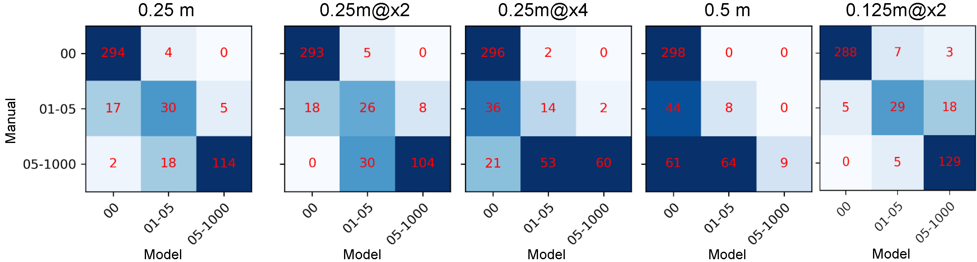
3.1. Grids of Boulder Density

Figure 5 displays boulder densities estimated by the model on original and upscaled validation mosaics and the expert interpretation. The corresponding confusion matrices are shown in Figure 6, while the precision, recall and F 1 scores are given in Table 1.
It is observed that the overall shape of the local boulder field is comparable between the model and the manual interpretation, both for the original mosaic and the 0.25 m @ × 2 mosaic. Visually, the shape of the boulder fields is more poorly preserved for the LR mosaic of 0.5 m and the 0.25 m @ × 4 mosaic. In case of the 1.0 m mosaic, only one grid cell including boulders is recognized by the model.
The manual detection yields 3170 detected boulders. Running on the validation mosaic at the native resolution of 0.25 m, the model finds 2704 boulders. The classification of the boulder grids yielded an F 1 score of 0.81, with similar precision and recall values of 0.82 and 0.81, respectively. The model run on the LR mosaic of 0.5 m resolution yields 353 detected boulders, while the F 1 score drops to 0.37. The strongly reduced number of detected boulders is mostly represented by the misclassification of dense boulder cells, of which only 9 out of 134 are found. At a mosaic resolution of 1.0 m, the model only identifies a single boulder in the validation area. The mosaic was excluded from further performance comparisons.
The 0.5 m and 1.0 m mosaics upscaled by SRResnet to 0.25 m resolution deliver improved results compared to the LR mosaics. The model run on the 0.25 m @ × 2 mosaic achieves an F 1 of 0.76 with 2333 identified objects. Little misclassification of empty cells take places, with 5 out of 298 cells being incorrectly assigned. The majority of wrong classifications is found in the intermediate class of 5–10 boulders. For the model running on the 0.25 m @ × 4 mosaic, the F 1 score is reduced to 0.58, with 884 identified boulders. The boulder density is being generally underestimated, represented by an reduced recall of 0.57. For the 0-block class, few false classifications occur (2 cells of 298).
Following the comparison with datasets where a native resolution mosaic is available, the backscatter mosaics were upscaled beyond the initially available resolution by a factor of two to a resolution of 0.125 m, and the automatic detection applied to image tiles of 25 × 25 m. In total, 4593 boulders are detected, 1423 more than the manual count at 0.25 m resolution. The F 1 score in comparison to the manual interpretation is 0.84, with nearly identical values for precision (0.85) and recall (0.83). The general shape of the area with dense boulders is preserved, but more numerous occurrences of boulders are observed in previously empty cells (Figure 5).

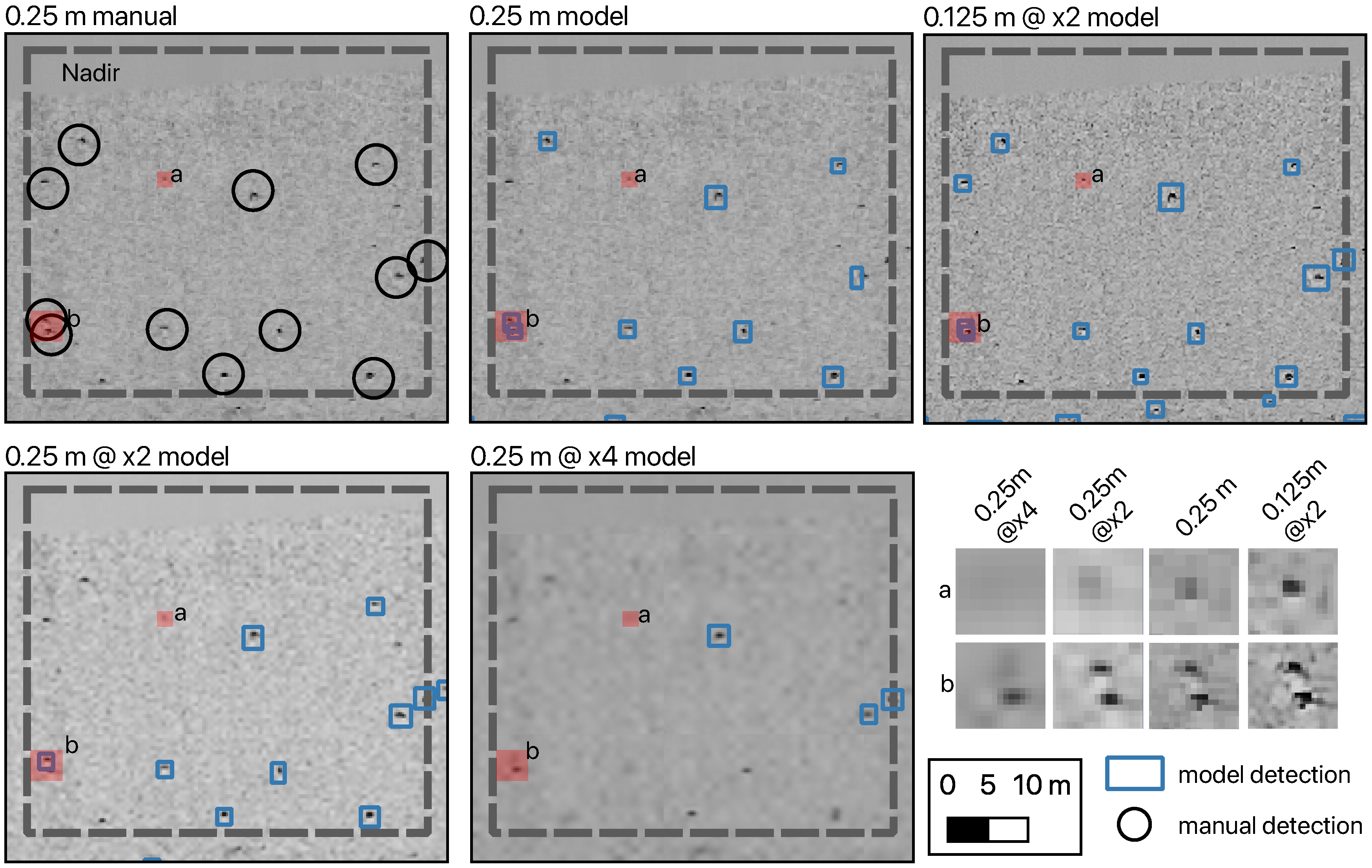
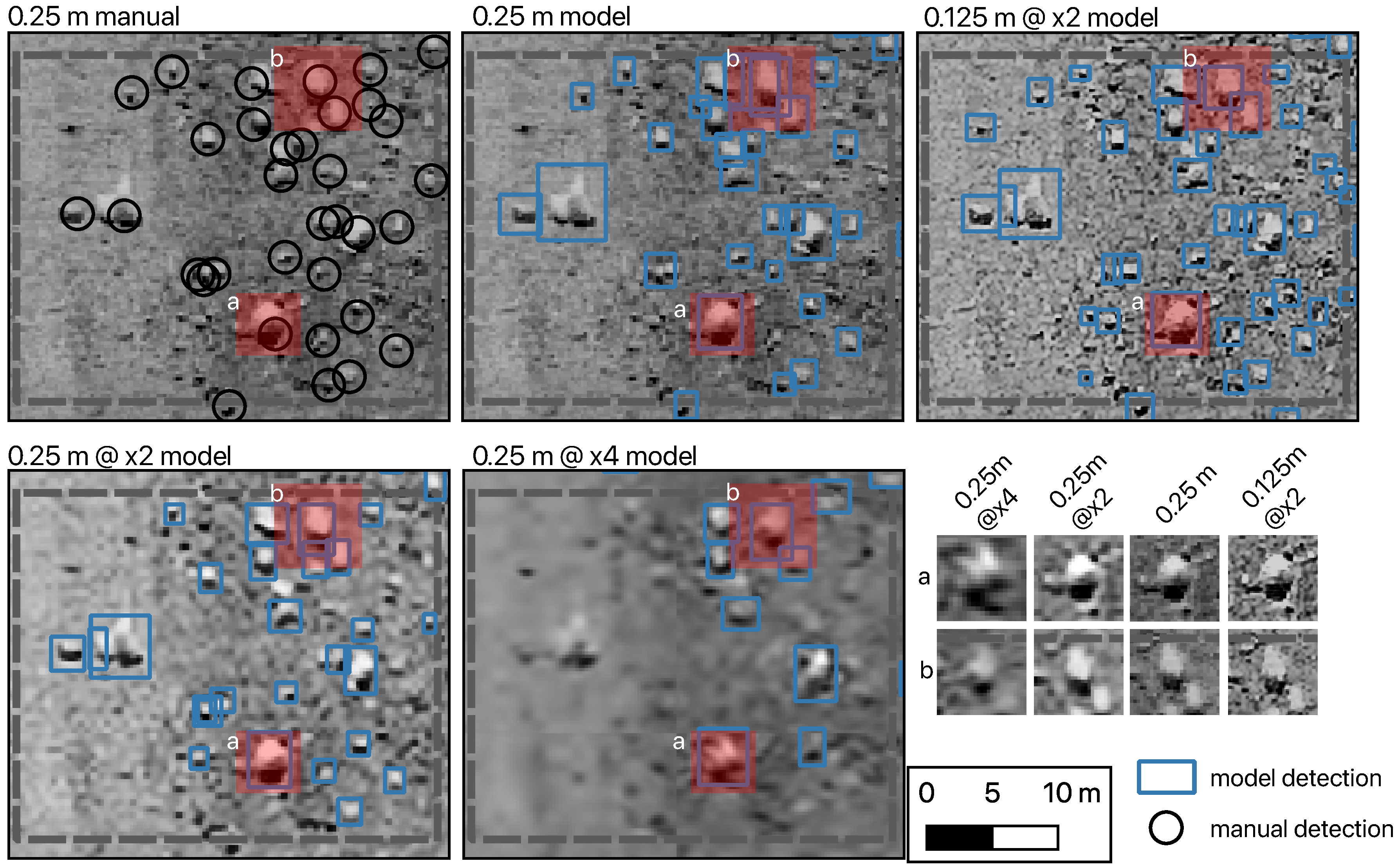
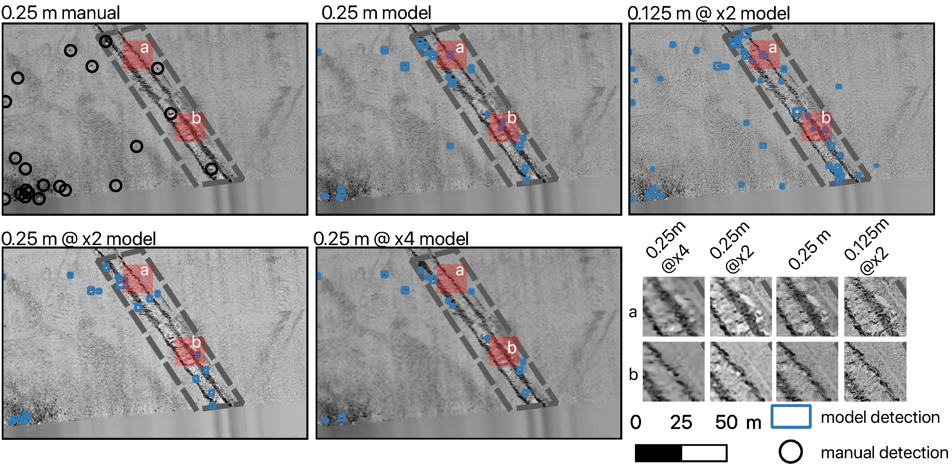
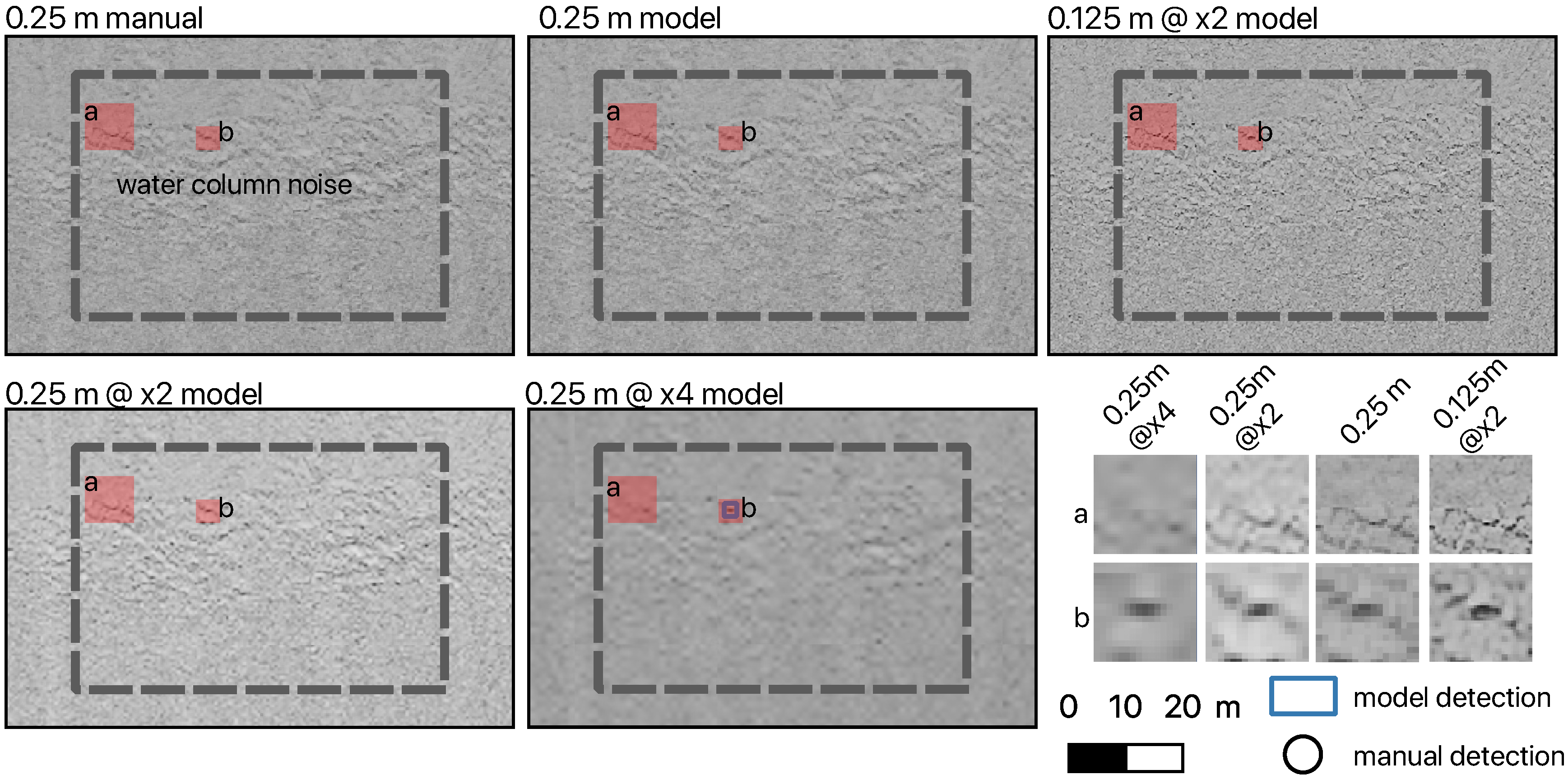
3.2. Boulder Detection Performance in Different Seafloor Facies

To assess the boulder detection performance on the upscaled mosaics depending on seafloor composition, the validation mosaic (Figure 1c) is differentiated into several facies. In the south-west and north-east, extended areas of homogeneous backscatter appearance are observed in medium grayscale intensities, comprized of mainly sandy material. Here, isolated boulders are recognized on the sandy material (Figure 7). In the north-western and south-eastern part, areas of generally high backscatter intensity with distinct boundaries to the surrounding seafloor are comprized of glacial lag deposits, widespread in the Baltic Sea, and numerous boulders of larger (Figure 8) and smaller (Figure 9) size are observed. Anthropogenic impact is expressed by an artificial plough mark, which is crossing the central part of the validation mosaic (Figure 10). Throughout the mosaic, two different artefacts are observed: Extensive blanking of side scan data occurs in the nadir, directly below the side scan sonar towfish (observed in Figure 7 and Figure 10). In addition, intense water column stratification effects are observed especially in the outer parts of the side scan sonar swaths (Figure 11). The corresponding accuracy numbers for all facies are given in Table 2.
For the facies of isolated boulders on homogeneous sand (Figure 7), no artefacts are introduced into the background during the upscaling, including the nadir region. In the original mosaic of 0.25 m resolution, 12 boulders are recognized. Two features which may be small boulders are missed by the model on the native mosaic, three are missed by the model on the 0.25 m @ × 2 mosaic, and nine are missed on the 0.25 m @ × 4 mosaic. No false positives are present for isolated small boulders on sandy seafloor. However, due to decreasing recall the F 1 score decreases slightly from 0.91 for the original mosaic to 0.86 for the image upscaled by a factor of 2, and drops to 0.4 for the image upscaled by a factor of 4. The detection run on the 0.125 m @ × 2 resolution mosaic finds 12 boulders, matching those found by manual interpretation of the 0.25 m mosaic. However, the increased resolution allows the manual identification of two additional boulders. The resulting F 1 score is 0.92 for the 0.125 m @ × 2 mosaic.
Figure 8 demonstrates the performance in an area including large boulders with distinct and extended shadows on glacial lag deposits. From west to east, the original image shows a gradual increase in backscatter, which is reproduced in images upscaled by a factor of 2 and 4. The manual count results in 32 boulders. The number of boulder recognized in the native mosaic by the model is 28 with an F 1 score of 0.85. The model running on the 0.25 m @ × 2 mosaic finds 26 objects, while the number drops to 9 for the 0.25 m @ × 4 mosaic. The respective F 1 scores are 0.75 and 0.44. For large boulders, the model counts 35 boulders on the 0.125 m @ × 2 mosaic, while 55 potential boulders could be identified manually at the increased resolution. Of these, 34 are also identified as boulders by the automatic classifications, while 21 manual interpretations are not confirmed by the model. The resulting F 1 score for the upscaled models is 0.77.
The case of numerous small boulder on a medium to high backscatter background is shown in Figure 9. From 42 boulders that are recognized manually, 29 are found by the model on the native mosaic (F 1 score 0.82), 26 on the 0.25 m @ × 2 mosaic (F 1 score 0.68) and 12 on the 0.25 m @ × 4 mosaic (F 1 score 0.41). The discrepancy between manually and automatically identified boulders on the upscaled mosaic increases for the facies of small boulders at 0.125 m @ × 2, with 82 manually identified boulder candidates. Of these, 54 are also found by the model, which in addition finds 5 false positive objects, resulting in an F 1 score of 0.77. For all three boulder facies, precision values remain at a comparable level to the interpretation of the native mosaic, while recall values decrease substantially.
The performance in areas of morphological features (plough marks) is shown in Figure 10. Within the plough marks, the number of detected boulders by the model exceeds the manual intepretation regardless of the underlying mosaic, resulting in F 1 scores around 0.4. A further increasing number of false positives detected by the model on the 0.125 m @ × 2 mosaic. Here, at maximum 5 potential boulders are manually identified, while 29 potential matches are found during the automatic classification. The corresponding low precision value of 0.1 cause a F 1 score of 0.17. The trend of an overestimation of boulders is observed all along the plough mark, continuing outside of the shown subset. Over the complete validation mosaic, 37 boulders are identified manually in the area with plough marks (1.2% of total detections), while 69 boulders are found by the model on the 0.25 m mosaic (2.6% of total detections), 80 on the 0.25 m @ × 2 mosaic (3.4% of total detections), 39 on the 0.25 m @ × 4 mosaic (4.4% of total detections) and 128 on the 0.125 m @ × 2 mosaic (2.7% of total detections). For the area with water column artefacts (as well as areas of the side scan sonar nadir), few misclassifications occur chiefly for the mosaic upscaled by a factor of 4, with an example shown in Figure 11.

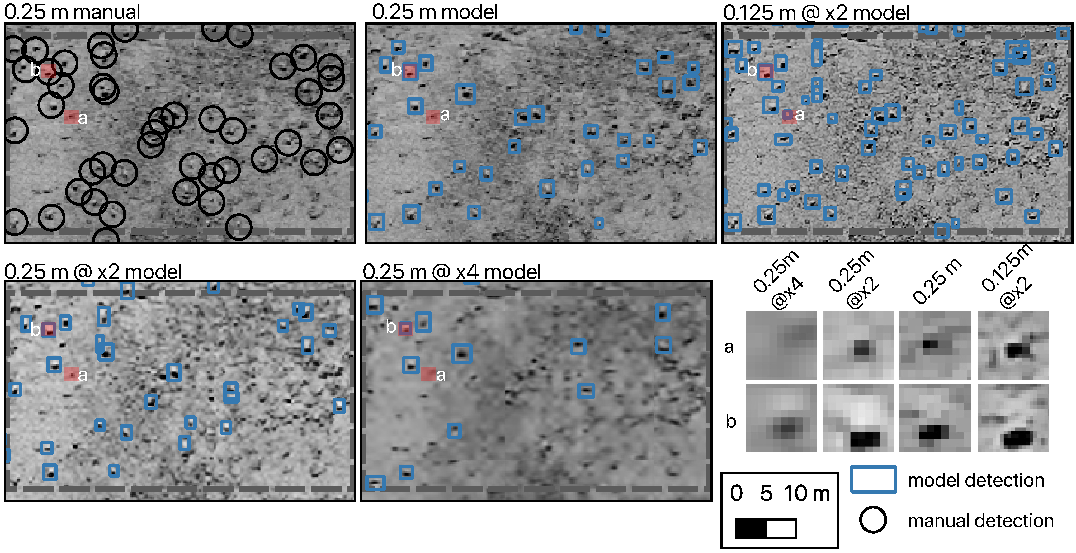
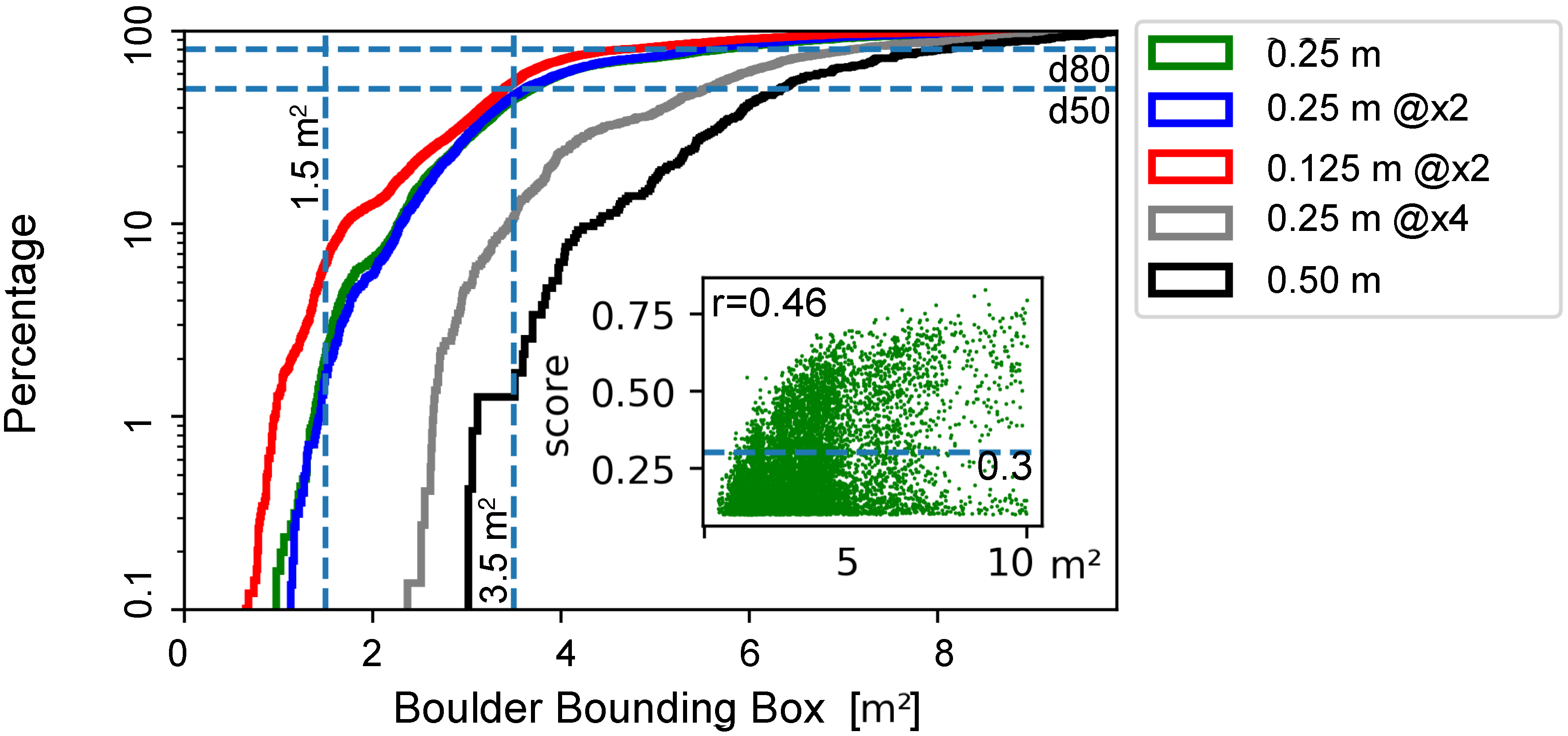
3.3. Small Object Detection

The detection of small objects, here assumed to correspond to small bounding boxes, is of special interest. To determine whether the upscaling improved the detection of small boulders, the areas covered by the bounding boxes are displayed in Figure 12 for the automatic boulder detection applied to the original and upscaled mosaics. The highest number of boulders is detected around 3.5 m 2 on the 0.25 m, 0.25 m @ × 2 and 0.125 m @ × 2 mosaics. These values roughly corresponds to the median of the bounding box size, which is 3.40 m 2 for the 0.125 m @ × 2, 3.69 m 2 for the 0.25 m and 3.62 m 2 for the 0.25 m @ × 2 mosaic. Generally, the distribution of the bounding box sizes is increasingly similar towards larger values for these mosaics, with negligible differences above the 80th percentile (Figure 12).
For the native mosaic at 0.25 m resolution, and the upscaled mosaic 0.25 m @ × 2 no significant difference in the relative distribution of smaller-sized bounding box dimensions is observed, although the absolute numbers of detected objects are larger for the model at native 0.25 m resolution. The minimum bounding box size is slightly lower for the native 0.25 m resolution, with a minimum of 0.93 m 2 , compared to 1.04 m 2 for the 0.25 m @ × 2 mosaic. However, the number of detected small objects with bounding boxes of less than 1.5 m 2 is limited to around 1% of the total detections, with 50 objects for the original validation mosaic and 35 objects for the mosaic upscaled to 0.25 m. The 0.125 m @ × 2 mosaic yields a higher number of smaller objects. The minimum detected object size is 0.53 m 2 and a total number of 303 potential boulders with bounding boxes less than 1.5 m 2 exist, corresponding to ca. 7% of the total number of detected objects.
In contrast, a clear drop of detected objects with small bounding boxes is observed for the 0.25 m @ × 4 mosaic and the LR mosaic of 0.5 m resolution. The former shows a median of 5.55 m 2 and a minimum detected bounding box size of 2.37 m 2 , the latter a median of 6.33 m 2 and a minimum detected bounding box size of 3.06 m 2 . For the 0.5 m mosaic, no bounding boxes with a size between 3 m 2 to 3.5 m 2 are present.
Figure 12 shows that a moderate correlation of 0.46 (p < 0.01) exists between the bounding box area and the threshold score assigned by the boulder detection model for the 0.25 m 2 model.

4. Discussion

4.1. Impact on Boulder Density Grids

The interpretation of marine acoustic data by automated methods remains challenging in many areas, including the identification of boulders [5]. The recent approach to better include boulders in marine spatial planning and meet demands of authorities is to classify boulders in grid cells of 50 × 50 m at a defined backscatter mosaic resolution of 0.25 m [5]. However, vast areas have been mapped at resolutions below 0.25 m in the German Baltic Sea and North Sea, and a re-surveying would be time consuming and expensive. In this regard, it is clearly observed that the super resolution followed by automated object detection is advantageous compared to using lower resolution images for both upscaling factors of 2 and 4, especially given the fast computation time of the trained models during the post-processing workflow. Especially the 0.5 m mosaics that are upscaled by a factor of 2 deliver a very close agreement to both manual counting and to model runs on the native 0.25 m resolution in this study, with F 1 scores of 0.76 and 0.81, respectively. It has to be considered that metrices were calculated very conservatively. Especially the assumption, that the true conditions are reflected in manual counting is not correct, and the actual performance of the models will be underestimated. The performance on the 0.25 m @ × 4 mosaic is noticeably poorer, compared to the native resolution. However, the increase in performance compared to the original low resolution model (from 1 to 884 detections) is clear, and the results outperform the low-resolution 0.5 m mosaic (Figure 2). The upscaling to 0.125 m brings a slight further improvement of the precision compared to the 0.25 m mosaic at native resolution. Recall and F 1 are not as meaningful for this comparison, as the total number of detected boulders increases in the higher resolution image. The higher precision exists despite several obviously false detections in empty cells, and the detection of isolated boulders in several previously empty cells. Figure 5a shows an example where a previously only faintly visibly object can be interpreted as a boulder following upscaling, causing a reclassification of the corresponding grid cell that is an improvement above the original classification. In contrast, Figure 5b displays an instance where a water column artefact is interpreted as a false positive following upscaling. It may be argued that the absence of false positive detections, i.e., a high precision, especially in empty cells is more important than a high recall of the actually available boulders, which is not possible to achieve. The precision in the zero boulder classes is above 0.9 in all cases, with less than 4% wrongly classified empty cells (Figure 6). This indicates, as also observed in Figure 11, that widespread water column stratification artefacts are not wrongly interpreted as objects following the upscaling procedure. In summary, for the creation of boulder density grids to the current standard of 0.25 m input mosaic resolution, it is suggested that a re-surveying of areas may not be necessary if data exists at least in a resolution of 0.5 m and can be upscaled. The upscaled mosaics deliver similar performance to the native resolution in this study. A noticeable drop in performance is observed when upscaling by a factor of 4, suggesting that mosaics of 1 m resolution are not suitable as a base for boulder detection.

4.2. Impact of Seafloor Facies

To better understand the range of seafloor facies where the upscaling and automatic detection is feasible, and for many applications, such as ecosystem research on reef structures [35] or determination of hard ground settlement area [36], the detection of individual boulders is required. Regarding the impact of different seafloor facies on individual boulder detection, a drop in performance towards more complex seafloor, with a higher number of smaller objects, is observed (Table 2). The drop in performance is chiefly controlled by a lack of recall, with the human expert continuously finding a higher number of objects compared to the automated detection. Especially for the 0.25 m @ × 4 mosaic, recall values remain at approximately 25% of the human interpretation. The performance of the 0.25 m @ × 2 mosaic is affected most in the area with many small boulders, indicating that the super resolution fails to restore very small, clustered objects, a trend that is commonly observed in other areas of application [17]. On the other hand, and important for practical application, few false positives are introduced and the precision exceeds 0.85 for all natural facies, and a drop in performance depending on the background sediment, as observed in previous studies using Haar-like features for boulder detection [3], was not observed. However, in contrast to the good performance on natural seafloor, many false positives around plough marks created by anthropogenic impact exist, comprising a noticeable percentage of the total number of detections by the model between 2% and 4%, depending on the mosaic. The problem is already prevalent in the native mosaic resolution of 0.25 m [8]. The poor performance is neither improved nor made worse by the upscaling procedure (Table 2). While further improvements of the training database to include more plough marks may improve performance, encoding additional information such as bathymetry or derived parameters such as the bathymetric positioning index as additional image channels should be pursued in the future, similar to the application of multispectral satellite images [16]. In the meantime, complex morphological areas such plough marks need to be manually quality checked for practical applications.

4.3. Impact on Small Object Detection

Next to the performance in complex seabed compositions, the challenge for individual boulder detection is that a large percentage of boulders (size class 26.5 cm to 4.1 m [37]) is by definition at or even below the pixel resolution of available acoustic mosaics, which are mostly available in resolutions of 1.0 to 0.25 m in the German Baltic Sea and North Sea. The recording of higher resolution data by MBES or SSS quickly becomes infeasible due to low ranges and required low ship speeds [19,22]. In addition, recent research demonstrates that the minimum boulder size which can be detected by acoustic remote sensing systematically depends on survey geometries [36], and thus a complete picture cannot be achieved. While statistics of boulder size distribution over larger areas are rare, it was found that the number of cobbles with less than 20 cm in diameter may exceed the number of cobbles and boulders larger than 20 cm by a factor of 6, and a relationship of ca. 10:1 exists between boulders and large boulders in the North Sea [38]. A generally similar relation may be expected in the Baltic Sea, since boulders in both seas originate from glacial ice advances [39], although the exact composition will be different depending on erosion, transport and source area of the boulders [40]. In any case, it may be expected that the majority of objects is located at the fine end of the boulder spectrum, and effort should made to detect as many small objects as possible without introducing an undue amount of false positives.
The expectation of an increasing number of small boulders is clearly not reflected in the bounding box distribution based on any of the considered mosaics (Figure 12). The decrease in small objects is not primarily related to anchor box parameters of the object detection framework. The smallest anchor box of 32 × 32 pixels corresponds at a standard threshold of areal overlap of 0.5 (not accounting for ratios setting) to a minimum object size of 23 × 23 pixels. Because sub-images of 25 m × 25 m were used as input images and were upscaled to 800 pixels height and width internally by RetinaNet, 23 × 23 pixels corresponds to a minimum area of ca. 0.5 m 2 in the input images regardless of mosaic resolution. At a score threshold of 0.3, the smallest objects identified on the 0.125 m @ × 2 mosaic (0.53 m 2 ) correspond to the theoretical minimum and small object detection may have benefited from smaller anchor boxes. Detections based on all other mosaics are not affected.
Instead, it is observed that the minimum bounding box size for the 0.125 m @ × 2, 0.25 m and 0.25 m @ × 2 mosaics correspond to ca. 4 × 4 to 6 × 6 pixels in the mosaics, with smaller objects not exceeding the score threshold of 0.3. This explains the six-fold increase of detected objects with bounding boxes smaller than 1.50 m 2 on the 0.125 m @ × 2 mosaic. Increased pixel number correlate to an increased score, with r = 0 . 46 over bounding boxes from 0 to 10 m 2 . Therefore, upscaling allows smaller objects to achieve higher scores and significantly more smaller objects are recognized on the 0.125 m @ × 2 mosaic. As demonstrated by the high precision values of the 0.125 m @ × 2 mosaic, this does not cause an undue increase of false positive detections.
For larger bounding boxes, the score values of detected boulders reach a plateau (r reduces to −0.15 considering only bounding boxes above 5 m 2 ), as the increased amount of pixels no longer contribute to better scores. Figure 12 also demonstrates that above 5 m 2 , an increasing distinction between objects with high and low scores exists. This explains that for large bounding boxes, roughly above the 80th percentile (Figure 12), no performance differences between the 0.125 m @ × 2, 0.25 m and 0.25 m @ × 2 mosaics are observed. Finally, it should be noted that the upscaling, beyond the native resolution of the dataset, to 0.125 m resolution also benefitted the manual determination of smaller boulders (e.g., Figure 9), indicating the human interpreter is still more efficient at detecting very small objects on the seafloor. However, with an increasing amount of recognized objects the manual detection becomes even more unfeasible over larger areas. For the 0.25 m @ × 4 mosaic, upscaling still increases performance above the 0.5 m resolution mosaic, but the performance for small objects altogether is poor, with the minimum detected object bounding box comprising 2.37 m 2 . It can be assumed that fine boulders are not sufficiently imaged in the 1.0 m resolved LR mosaic, and cannot be restored by upscaling. Examples of fine boulders disappearing in the 0.25 m @ × 4 mosaics are displayed in Figure 7a and Figure 9a. In summary, upscaling by a factor of 2 causes a marked improvement in the detection of fine boulders, while no performance difference is observed for larger objects. However, the expected distribution of bounding box sizes, with a maximum at the smallest objects, is not achieved.

5. Conclusions

For the purpose of boulder detection, upscaling of backscatter mosaics by a factor of 2 clearly improved the results both for the creation of boulder density grids and small object detection. Regarding the continued use of older mosaics (map once, use many times), it is suggested that 0.5 m mosaics may be sufficient to locate boulder fields in the geological setting of the Baltic Sea, where boulders are typically densely packed. Mosaics of 1.0 m resolution (requiring an upscaling factor of 4) are found unsuitable for this purpose. However, with the model and training database used in this study, a quality check by human experts is required in morphologically complex areas of strong anthropogenic impacts. These areas require tuning of object detection models, the application of more advanced model architectures and consideration of bathymetric information in the future.

Supplementary Materials

The following materials S1 to S4 are available online at https://www.mdpi.com/2072-4292/12/14/2284/s1, Figure S1: Manual identification of boulders at 0.125 m for the facies isolated boulders, small boulders and large boulders. Figure S2: Zipped georeferenced training mosaics, Figure S3: zipped georeferenced validation mosaics, Figure S4: Used training database with coordinates of boulders used for training of the object detection model in sqlite format. RetinaNet is available at github.com/fizyr/keras-retinanet, last accessed 20.04.2020. The implementation of SRResnet can be found at github.com/brade31919/SRGAN-tensorflow, last accessed 04.06.2020. The repository for the anchor optimization is available at github.com/martinzlocha/anchor-optimization, last accessed 06.05.2020. The gdal utilities are available at gdal.org, last accessed 14.04.2020. Scikit-image is available at scikit-image.org, last accessed 14.04.2020.

Funding

This research received no external funding.

Acknowledgments

The author thanks Gitta von Rönn (CAU Kiel), Svenja Papenmeier (IOW) and Agata Feldens (IOW) for discussion on the subject. Franz Tauber (IOW, retired) processed the side scan sonar mosaics. Critical and encouraging comments of five anonymous reviewers improved the manuscript. The publication of this article was funded by the Open Access Fund of the Leibniz Association.

Conflicts of Interest

The author declares no conflict of interest.

References

  1. Anwar, S.; Khan, S.; Barnes, N. A Deep Journey into Super-resolution: A survey. ACM Comput. Surv. 2020, 53, 60:1–60:34. [Google Scholar] [CrossRef]
  2. Michaelis, R.; Hass, H.C.; Mielck, F.; Papenmeier, S.; Sander, L.; Ebbe, B.; Gutow, L.; Wiltshire, K.H. Hard-substrate habitats in the German Bight (South-Eastern North Sea) observed using drift videos. J. Sea Res. 2019, 144, 78–84. [Google Scholar] [CrossRef]
  3. Michaelis, R.; Hass, H.C.; Papenmeier, S.; Wiltshire, K.H. Automated Stone Detection on Side-Scan Sonar Mosaics Using Haar-Like Features. Geosciences 2019, 9, 216. [Google Scholar] [CrossRef] [Green Version]
  4. Papenmeier, S.; Hass, H.C. Detection of Stones in Marine Habitats Combining Simultaneous Hydroacoustic Surveys. Geosciences 2018, 8, 279. [Google Scholar] [CrossRef] [Green Version]
  5. Papenmeier, S.; Darr, A.; Feldens, P.; Michaelis, R. Hydroacoustic Mapping of Geogenic Hard Substrates: Challenges and Review of German Approaches. Geosciences 2020, 10, 100. [Google Scholar] [CrossRef] [Green Version]
  6. Brown, C.J.; Blondel, P. Developments in the application of multibeam sonar backscatter for seafloor habitat mapping. Appl. Acoust. 2009, 70, 1242–1247. [Google Scholar] [CrossRef]
  7. Wei, B.; Zhou, T.; Li, H.; Xing, T.; Li, Y. Theoretical and experimental study on multibeam synthetic aperture sonar. J. Acoust. Soc. Am. 2019, 145, 3177. [Google Scholar] [CrossRef]
  8. Feldens, P.; Darr, A.; Feldens, A.; Tauber, F. Detection of Boulders in Side Scan Sonar Mosaics by a Neural Network. Geosciences 2019, 9, 159. [Google Scholar] [CrossRef] [Green Version]
  9. Ren, Y.; Zhu, C.; Xiao, S. Small Object Detection in Optical Remote Sensing Images via Modified Faster R-CNN. Appl. Sci. 2018, 8, 813. [Google Scholar] [CrossRef] [Green Version]
  10. Chen, X.; Andersen, T.J.; Morono, Y.; Inagaki, F.; Jørgensen, B.B.; Lever, M.A. Bioturbation as a key driver behind the dominance of Bacteria over Archaea in near-surface sediment. Sci. Rep. 2017, 7, 1–14. [Google Scholar] [CrossRef]
  11. Eggert, C.; Zecha, D.; Brehm, S.; Lienhart, R. Improving Small Object Proposals for Company Logo Detection. In Proceedings of the 2017 ACM on International Conference on Multimedia Retrieval—ICMR ‘17, Bucharest, Romania, 6–9 June 2017; pp. 167–174. [Google Scholar]
  12. Zhang, L.; Zhang, L.; Du, B. Deep Learning for Remote Sensing Data: A Technical Tutorial on the State of the Art. IEEE Geosci. Remote. Sens. Mag. 2016, 4, 22–40. [Google Scholar] [CrossRef]
  13. Yue, L.; Shen, H.; Li, J.; Yuan, Q.; Zhang, H.; Zhang, L. Image super-resolution: The techniques, applications, and future. Signal Process. 2016, 128, 389–408. [Google Scholar] [CrossRef]
  14. Dong, C.; Loy, C.C.; He, K.; Tang, X. Image Super-Resolution Using Deep Convolutional Networks. IEEE Trans. Pattern Anal. Mach. Intell. 2016, 38, 295–307. [Google Scholar] [CrossRef] [Green Version]
  15. Wang, Z.; Chen, J.; Hoi, S.C.H. Deep Learning for Image Super-resolution: A Survey. IEEE Trans. Pattern Anal. Mach. Intell. 2020. [Google Scholar] [CrossRef] [Green Version]
  16. Liebel, L.; Körner, M. Single-Image Super Resolution For Multispectral Remote Sensing Data Using Convolutional Neural Networks. Int. Arch. Photogramm. Remote. Sens. Spat. Inf. Sci. 2016, XLI-B3, 883–890. [Google Scholar] [CrossRef]
  17. Shermeyer, J.; Van Etten, A. The effects of super-resolution on object detection performance in satellite imagery. In Proceedings of the IEEE Conference on Computer Vision and Pattern Recognition Workshops, Long Beach, CA, USA, 16–20 June 2019. [Google Scholar]
  18. Blondel, P. The Handbook of Sidescan Sonar; Springer: Berlin, Germany; New York, NY, USA; Chichester, UK, 2009; p. 316. [Google Scholar]
  19. Lurton, X.; Lamarche, G.; Brown, C.; Lucieer, V.; Rice, G.; Schimel, A.; Weber, T. Backscatter Measurements by Seafloor-Mapping Sonars Guidelines and Recommendations. 2015. Available online: http://geohab.org/wp-content/uploads/2018/09/BWSG-REPORT-MAY2015.pdf (accessed on 5 June 2020).
  20. Wilken, D.; Feldens, P.; Wunderlich, T.; Heinrich, C. Application of 2D Fourier filtering for elimination of stripe noise in side-scan sonar mosaics. Geo Mar. Lett. 2012, 32, 337–347. [Google Scholar] [CrossRef]
  21. Lamarche, G.; Lurton, X.; Verdier, A.L.; Augustin, J.M. Quantitative characterisation of seafloor substrate and bedforms using advanced processing of multibeam backscatter—Application to Cook Strait, New Zealand. Cont. Shelf Res. 2011, 31, S93–S109. [Google Scholar] [CrossRef] [Green Version]
  22. BSH. Guideline for Seafloor Mapping in German Marine Waters Using High-Resolution Sonars. BSH No. 7201. 2016, p. 147. Available online: https://www.bsh.de/DE/PUBLIKATIONEN/_Anlagen/Downloads/Meer_und_Umwelt/Weitere_Publikationen/Guideline-for-Seafloor-Mapping.html (accessed on 5 June 2020).
  23. Feldens, P.; Schwarzer, K. The Ancylus Lake stage of the Baltic Sea in Fehmarn Belt: Indications of a new threshold. Cont. Shelf Res. 2012, 35, 43–52. [Google Scholar] [CrossRef]
  24. Heinrich, C.; Anders, S.; Schwarzer, K. Late Pleistocene and early Holocene drainage events in the eastern Fehmarn Belt and Mecklenburg Bight, SW Baltic Sea. Boreas 2018, 47, 754–767. [Google Scholar] [CrossRef] [Green Version]
  25. Lemke, W.; Kuijpers, A.; Hoffmann, G.; Milkert, D.; Atzler, R. The Darss Sill, hydrographic threshold in the southwestern Baltic: Late Quaternary geology and recent sediment dynamics. Cont. Shelf Res. 1994, 14, 847–870. [Google Scholar] [CrossRef] [Green Version]
  26. Nielsen, E.P.; Jensen, J.; M, B.; Lomholt, S.; Kuijpers, A. Marine aggregates in the Danish sector of the Baltic Sea: Geological setting, exploitation potential and environmental assessment. Z. FüR Angew. Geol. 2004, NS2, 87–109. [Google Scholar]
  27. Ledig, C.; Theis, L.; Huszar, F.; Caballero, J.; Cunningham, A.; Acosta, A.; Aitken, A.; Tejani, A.; Totz, J.; Wang, Z.; et al. Photo-Realistic Single Image Super-Resolution Using a Generative Adversarial Network. In Proceedings of the IEEE Conference on Computer Vision and Pattern Recognition (CVPR), Honolulu, HI, USA, 21–26 July 2017; pp. 4681–4690. [Google Scholar]
  28. Shi, W.; Caballero, J.; Huszár, F.; Totz, J.; Aitken, A.P.; Bishop, R.; Rueckert, D.; Wang, Z. Real-Time Single Image and Video Super-Resolution Using an Efficient Sub-Pixel Convolutional Neural Network. In Proceedings of the IEEE Conference on Computer Vision and Pattern Recognition (CVPR), Las Vegas, NV, USA, 27–30 June 2016; pp. 1874–1883. [Google Scholar]
  29. Van der Walt, S.; Schönberger, J.L.; Nunez-Iglesias, J.; Boulogne, F.; Warner, J.D.; Yager, N.; Gouillart, E.; Yu, T. scikit-image: Image processing in Python. PeerJ 2014, 2, e453. [Google Scholar] [CrossRef] [PubMed]
  30. Kingma, D.P.; Ba, J. Adam: A method for stochastic optimization. arXiv 2014, arXiv:1412.6980. [Google Scholar]
  31. Aitken, A.; Ledig, C.; Theis, L.; Caballero, J.; Wang, Z.; Shi, W. Checkerboard artifact free sub-pixel convolution: A note on sub-pixel convolution, resize convolution and convolution resize. arXiv 2017, arXiv:1707.02937. [Google Scholar]
  32. Lin, T.Y.; Goyal, P.; Girshick, R.; He, K.; Dollár, P. Focal Loss for Dense Object Detection. In Proceedings of the IEEE International Conference on Computer Vision (ICCV), Venice, Italy, 22–29 October 2017; pp. 2980–2988. [Google Scholar]
  33. Zlocha, M.; Dou, Q.; Glocker, B. Improving RetinaNet for CT Lesion Detection with Dense Masks from Weak RECIST Labels. In International Conference on Medical Image Computing and Computer-Assisted Intervention; Springer: Cham, Germany, 2019; pp. 402–410. [Google Scholar]
  34. Pedregosa, F.; Varoquaux, G.; Gramfort, A.; Michel, V.; Thirion, B.; Grisel, O.; Blondel, M.; Prettenhofer, P.; Weiss, R.; Dubourg, V.; et al. Scikit-learn: Machine Learning in Python. J. Mach. Learn. Res. 2011, 12, 2825–2830. [Google Scholar]
  35. Beisiegel, K.; Darr, A.; Zettler, M.L.; Friedland, R.; Gräwe, U.; Gogina, M. Understanding the spatial distribution of subtidal reef assemblages in the southern Baltic Sea using towed camera platform imagery. Estuarine Coast. Shelf Sci. 2018, 207, 82–92. [Google Scholar] [CrossRef]
  36. Rönn, G.A.V.; Schwarzer, K.; Reimers, H.C.; Winter, C. Limitations of Boulder Detection in Shallow Water Habitats Using High-Resolution Sidescan Sonar Images. Geosciences 2019, 9, 390. [Google Scholar] [CrossRef] [Green Version]
  37. Terry, J.; Goff, J. Megaclasts: Proposed Revised Nomenclature At the Coarse End of the Udden-Wentworth Grain-Size Scale for Sedimentary Particles. J. Sediment. Res. 2014, 84, 192–197. [Google Scholar] [CrossRef]
  38. Michaelis, R.; Hass, H.C.; Mielck, F.; Papenmeier, S.; Sander, L.; Gutow, L.; Wiltshire, K.H. Epibenthic assemblages of hard-substrate habitats in the German Bight (south-eastern North Sea) described using drift videos. Cont. Shelf Res. 2019, 175, 30–41. [Google Scholar] [CrossRef]
  39. Diesing, M.; Schwarzer, K. Identification of submarine hard-bottom substrates in the German North Sea and Baltic Sea EEZ with high-resolution acoustic seafloor imaging. In Progress in Marine Conservation in Europe; Springer: Berlin/Heidelberg, Germany, 2006; pp. 111–125. [Google Scholar]
  40. Haldorsen, S. Grain-size distribution of subglacial till and its relstion to glacial crushing and abrasion. Boreas 1981, 10, 91–105. [Google Scholar] [CrossRef]
Figure 1. (a) Location of the mosaics used for validation and training of the super resolution and object detection model. Areal extension of mosaics is enlarged. (b) Validation mosaic. (c) Annotated validation mosaic. (d) Mosaics used for training of the super resolution model. (e) Mosaic used for training of the object detection model. The mosaic was also part of the super-resolution training suite. The native resolution of all mosaics is 0.25 m. Colors in (ae) correspond to the depth scale.
Remotesensing 12 02284 g001
Figure 2. (a) Simplified structure of the used model based on [27,28]. (b) A schematic sketch of the upscaling procedure by pixel shuffling with an upscaling factor of 2 for a single-channel image is given in the lower right. The following abbreviations are used in a and b: c the number of channels of the input and output images and the intermediate feature maps; Conv convolutional layer; BN batch normalization layer; ReLu rectified linear activation unit; Sum Layer that elementwise sums the output of a residual block with the output of the prior residual block; PS(r) Upscaling by periodic pixel shuffling with the upscaling factor r; H image height; W image width.
Remotesensing 12 02284 g002
Figure 3. Workflow followed during training of SRResnet (a) and RetinaNet (b).
Remotesensing 12 02284 g003
Figure 4. Example of a sub-image located at 54.9896°N, 13.1335°E at the different pixel dimensions. For better visualization, all images are magnified from the original size by a factor of 5. The 25 × 25 pixel LR image was magnified by a factor of 10 instead. The boulders are recognized by typical backscatter patterns, with high backscatter intensities facing the side scan sonar towfish, and acoustic shadows on the opposite side. It is observed that the image upscaled by a factor of 2 shows a slight increase in average greylevel intensities.
Remotesensing 12 02284 g004
Figure 5. Block densities of the validation area for manual interpretation and the model running on different mosaics. (a) hows an example where a grid cell classification changed after correctly identifying a small boulder following upscaling to 0.125 m resolution. (b) shows an example where a grid cell classification changed due to mis-interpretation of water column stratification after upscaling to 0.125 m resolution.
Remotesensing 12 02284 g005
Figure 6. Confusion matrices of the block diagrams shown in Figure 5.
Remotesensing 12 02284 g006
Figure 7. Subsets of the native and upscaled mosaics for the isolated boulder facies. Manual and model detections are marked. Insets detail the appearance of individual boulders in the different mosaics. The location of the shown mosaic subset in the validation mosaic is marked in Figure 1.
Remotesensing 12 02284 g007
Figure 8. Subsets of the native and upscaled mosaics for the large boulder facies. Manual and model detections are marked. Insets detail the appearance of individual boulders in the different mosaics. The location of the shown mosaic subset in the validation mosaic is marked in Figure 1.
Remotesensing 12 02284 g008
Figure 9. Subsets of the native and upscaled mosaics for the small boulder facies. Manual and model detections are marked. Insets detail the appearance of individual boulders in the different mosaics. The location of the shown mosaic subset in the validation mosaic is marked in Figure 1.
Remotesensing 12 02284 g009
Figure 10. Subsets of the native and upscaled mosaics in an area of plough marks. Manual and model detections are marked. Insets detail the appearance of the plough mark boundaries in the different mosaics. The location of the shown mosaic subset in the validation mosaic is marked in Figure 1.
Remotesensing 12 02284 g010
Figure 11. Subsets of the native and upscaled mosaics in an area affected by water column stratification artefacts. Insets detail the appearance of the water column artefacts in the different mosaics. The location of the shown mosaic subset in the validation mosaic is marked in Figure 1.
Remotesensing 12 02284 g011
Figure 12. Cumulative area distribution of bounding boxes from 0 m 2 to 10 m 2 . The scatter plot inset demonstrates the correlation between bounding box area and object score. The score threshold of 0.3 is indicated by a dashed blue line.
Remotesensing 12 02284 g012
Table 1. Precision, accuracy and F 1 score (macro-average) for boulder densities displayed in Figure 5.
MosaicBoulder CountPrecisionRecallF 1
Mosaic manual3170---
Mosaic 0.25 m resolution27040.820.800.81
Mosaic 0.5 m resolution3530.620.410.37
Mosaic 0.125 m @ × 245930.850.830.84
Mosaic 0.25 m @ × 223330.770.750.76
Mosaic 0.25 m @ × 48840.670.570.58
Table 2. Comparison of the automated boulder detection to the manual interpretation for the different facies and mosaics shown in Figure 7, Figure 8, Figure 9 and Figure 10.
MosaicFaciesManual CountModel CountTPFNFPPrecisionRecallF 1
Mosaic 0.25 misolated121010201.00.830.91
Mosaic 0.25 m @ × 2isolated99301.00.750.86
Mosaic 0.25 m @ × 4isolated33901.00.250.4
Mosaic 0.125 m @ × 2isolated141212201.00.860.92
Mosaic 0.25 mlarge322825630.890.810.85
Mosaic 0.25m @ × 2large26221140.850.670.75
Mosaic 0.25 m @ × 4large992301.00.280.44
Mosaic 0.125 m @ × 2large5535342110.970.640.77
Mosaic 0.25 msmall4229281410.970.670.82
Mosaic 0.25 m @ × 2small26231930.880.550.68
Mosaic 0.25 m @ × 4small12113110.920.260.41
Mosaic 0.125 m @ × 2small8259542850.920.660.77
Mosaic 0.25 mplough4123190.250.750.38
Mosaic 0.25 m @ × 2plough123190.250.750.38
Mosaic 0.25 m @ × 4plough103170.30.750.43
Mosaic 0.125 m @ × 2plough52932260.100.60.17

