Article

Soil Conservation Service Spatiotemporal Variability and Its Driving Mechanism on the Guizhou Plateau, China

1
Key Laboratory of Land Surface Patterns and Simulation, Institute of Geographic Science and Natural Resources Research, CAS, No.11, Datun Road, Chaoyang District, Beijing 100101, China
2
College of Resources and Environment, University of Chinese Academy of Sciences, No.19, Yuquan Road, Shijingshan District, Beijing 101407, China
*
Author to whom correspondence should be addressed.
Remote Sens. 2020, 12(14), 2187; https://doi.org/10.3390/rs12142187
Submission received: 31 May 2020 / Revised: 5 July 2020 / Accepted: 7 July 2020 / Published: 8 July 2020
(This article belongs to the Special Issue Remote Sensing of Soil Erosion)

Abstract

:
The Guizhou Plateau has an extremely fragile ecological environment with prominent soil and water losses. Since 2000, conservation policies and ecological restoration projects, e.g., the Grain for Green Project (GGP), have been implemented on the Guizhou Plateau to control soil/water losses which have achieved notable accomplishments. Using the Revised Universal Soil Loss Equation (RUSLE) to estimate the soil conservation service (SCS) on the Guizhou Plateau, this study analyzed the dynamic characteristics of its spatiotemporal variation based on multiyear (2000–2018) meteorological and remote sensing data to determine its driving mechanisms. Residual analysis of the meteorological and remote sensing data was used to evaluate the effect of anthropogenic activities. Results showed a clear upward trend (1.39 t ha−1 yr−1) of SCS on the Guizhou Plateau during 2000–2018, and areas with a highly improved positive effect on SCS were distributed primarily in karst landform regions. Precipitation and vegetation fractional coverage (VFC) were found to be positively correlated with SCS on the Guizhou Plateau. Specifically, the highest proportion of significant positive correlation between precipitation and SCS was related to the Wildlife Conservation Nature Reserve (WCNR), and the highest proportion of significant positive correlation between VFC and SCS was related to the GGP, i.e., 76.59% and 53.02%, respectively. Residual analysis revealed a significant positive role of anthropogenic activity on SCS improvement via ecological engineering in areas with a poor ecological background, e.g., the GGP in western areas where the ecological environment is fragile and the problem of water/soil loss is serious. In areas with a more robust ecological background, e.g., the engineering area of the WCNR, the effect of anthropogenic activity has had a largely negative effect on SCS. The findings of this study could make an important contribution to the development of ecological management projects and the work to control soil/water losses on the Guizhou Plateau.

Graphical Abstract

1. Introduction

The soil conservation service (SCS), which is an important regulating service of ecosystem services [1], plays a critical role in both the conservation of water and soil and the improvement of soil structure through ground cover and litter [2]. SCS provides not only an important foundation for human agricultural production, but also protection against the risk of flooding and deterioration of the ecological environment [3,4]. Aggravation of soil erosion can lead to serious soil and water losses, that result in ecosystem fragmentation and decline in both soil fertility and land quality [5], which could be detrimental to the ecological environment and the development of human society. Therefore, SCS evaluation is an important aspect in ecosystem service analysis.
The difference between the potential soil erosion and actual soil erosion can be used as a quantitative indicator of SCS [6]. In recent years, this method has been used widely to evaluate SCS on watersheds [7], regional [8], and other scales. This model is also particularly useful for simulating the dynamic changes of SCS under the effects of climatic and land use changes [9,10]. Many models have been proposed for the calculation of soil erosion. The United States Department of Agriculture proposed the Water Erosion Prediction Project model, which is a physical process model that can dynamically monitor the slope erosion process [11]; Morgan et al. [12] proposed the European soil erosion model, which divided the soil erosion instead of erosion between fine trenches and fine trenches is applied to the prediction of secondary rainfall erosion; De Roo et al. [13] proposed the Dutch soil erosion prediction model, which considers various processes in simulation of the process of soil erosion. The Revised Universal Soil Loss Equation (RUSLE) [11], issued by the United States Department of Agriculture, can be used for the assessment of soil erosion loss. In comparison with many other models, the RUSLE model has a simpler structure, a clearer physical meaning of parameters, and stronger practicable and comprehensive capabilities [14]. Ganasri and Ramesh [15] used the RUSLE model to estimate the amount of soil erosion in the Nethravathi Basin of southern India. Wu et al. [16] assessed the magnitude of soil erosion and its spatial distribution characteristics in the Mekong Basin. Wang et al. [17] studied soil erosion in the water source area of Shaanxi (China) using the RULSE model. The increased use of geographic information systems (GIS) and remote sensing (RS) technology has allowed the evaluation of ecological services to be supported by long-term dynamic information [18]. Li and Zheng [19] studied soil erosion changes during 2001–2010 in the Yanhe watershed on the Loess Plateau (China) with GIS and RS support. Wang et al. [20] investigated the degree of soil erosion in the area of the Three Gorges Reservoir (China) during 2000–2010 using the RUSLE model in conjunction with a Moderate-resolution Imaging Spectroradiometer (MODIS) normalized difference vegetation index (NDVI) map and digital elevation model (DEM) data. Olorunfemi et al. [21] assessed potential soil erosion in Ekiti State (Nigeria) with a GIS platform and monthly rainfall data interpolated from climate point data using the inverse distance weighting method. The common data sources of RUSLE-based models are meteorological and RS data [22].
Topography is an important factor that affects the area and distribution of soil erosion, and slope has important influence on the mechanical composition of soil and runoff [23,24]. Slope-based runoff experimental methods [25] for measuring soil erosion tend to be elaborate, so cannot be used for large-scale simulation studies. When using prediction methods such as the RUSLE model, the accuracy of the topographical factor is extremely important. Although a DEM can represent an effective source of GIS-based topographic information, the topographical factor extracted from DEMs at different scales can affect the accuracy of the final soil erosion calculation results [26]. Consequently, the scale of DEM data should be selected depending on the scale and objectives of any particular study [27]. For large-scale study areas, the use of low-resolution DEM data would erase certain details of the surface terrain, thereby affecting the accuracy of the topographical factor. Conversely, the use of high-resolution data would exacerbate problems associated with the storage and processing of large volumes of data. In addition, for small-scale soil erosion studies and hydrologic-level analyses, it can be necessary to build very high resolution DEMs, even to runoff plot or hydrological observation scale [28]. Currently, satellite-derived high-resolution RS imagery (e.g., from the Sentinel 2A satellite) and DEMs acquired using unmanned aerial vehicle technology can be incorporated in quantitative studies of soil erosion [29].
Climate change and anthropogenic activities have altered the structure and function of ecosystems. Related studies have shown that global soil erosion is at increased risk under the influence of climate change and unrestrained anthropogenic activities [30]. Anthropogenic activity is the main driving factor affecting soil conservation that can change soil erosion [31]. Residual analysis is often used to study the driving mechanisms or to evaluate the impact of anthropogenic activities. For example, Wu et al. [32] undertook a quantitative assessment of the impact of weather conditions on air quality in Hohhot (China) using residual analysis. Luo et al. [33] also used residual analysis with MODIS-NDVI data to analyze the effect of climate change and anthropogenic activities on vegetation on the island of Hainan (China).
China is among the countries within which the problem of soil erosion is most serious. By 2011, the total area of land within China affected by soil erosion had reached 294.92 × 10⁴ km2 [34]. However, strengthening ecological awareness has led China to implement ecological engineering projects for comprehensive control of soil and water losses, e.g., the Shelterbelt Forest Project (SFP), Grain for Green Project (GGP), and Comprehensive Control Project of Rocky Desertification (CCPRD) [35]. Previous research has shown that ecological projects such as GGP could control soil erosion [36]. However, previous studies have not examined the spatiotemporal response of SCS to ecological engineering activities in regions with different landforms, especially in the karst areas. Moreover, few quantitative studies have investigated the roles of climate change (e.g., in relation to rainfall) and anthropogenic activities in driving SCS under the background of ecological engineering. These subjects are of great importance with regard to further improvement of the layout and implementation of ecological engineering constructions and projects for soil erosion control in specific areas.
The Guizhou Plateau, which is one of the regions of China with the most serious soil and water losses, has an extremely fragile ecological environment. It is a region characterized by its typical karst landforms, rocky desertification, and serious soil erosion; the area of soil/water losses accounts for 43.5% of the total area [37]. The Guizhou Plateau, which is located at the confluence of the Yangtze and Pearl rivers, is an important ecological defense in the upper reaches of both river basins. Soil erosion within this region is related directly to the ecological security of the river basins and has considerable impact on the socioeconomic development of downstream areas. To improve the increasingly prominent problems of soil erosion and rocky desertification on the Guizhou Plateau, ecological restoration projects such as the CCPRD have been undertaken on a large scale since 2004 [38]. Zhang et al. [39] quantified the contribution rate of anthropogenic activities to vegetation coverage on the Guizhou Plateau under the effects of ecological engineering construction. It was found that the positive effects of anthropogenic activities outweighed the negative effects. Based on studies in the Shaanxi region of China, Liu et al. [40] concluded that GGP implementation has reduced soil erosion and enhanced the soil protection effect. The implementation of large-scale ecological projects raises certain important scientific concerns. For example, it is imperative to ascertain the changes that have taken place in terms of SCS on the Guizhou Plateau, determine the characteristics of SCS on the Guizhou Plateau under different ecological engineering constructions, examine the impact of ecological engineering on SCS, establish the characteristics of SCS in regions with different landforms regions, and investigate whether ecological engineering construction has been adapted sufficiently to local conditions.
The Guizhou Plateau is located in the largest karst area in the world, where population pressure is greatest, land degradation serious, and rocky desertification prominent. Consequently, the ecological restoration of land degradation characterized by soil erosion is a difficult problem [41]. The fragile ecological environment of the Guizhou Plateau makes it highly susceptible to the effects of anthropogenic activities. China has implemented many ecological projects in this region. However, few studies have considered the spatiotemporal variation and driving factors of SCS in relation to ecological engineering construction on the Guizhou Plateau.
This study analyzed the spatiotemporal variation and driving factors of SCS on the Guizhou Plateau during 2000–2018 using GIS in combination with long-term meteorological and RS data. First, the RUSLE model was used to calculate SCS. Then, the comparative influence of natural factors (e.g., precipitation and vegetation fractional coverage (VFC)) and anthropogenic activities on SCS was determined through regression analysis and residual analysis, following which the evolution trend of SCS and the effect of different ecological engineering projects on SCS were assessed. The objectives of this study were to evaluate the variability of SCS on the Guizhou Plateau during 2000–2018, elucidate its driving mechanisms, clarify the effects of anthropogenic activities under ecological restoration projects in regions with different landforms, and propose suggestions for reducing soil erosion and rational planning of ecological engineering areas. The findings will make an important contribution to both the work of controlling soil and water losses on the Guizhou Plateau area and the development of an ecologically aware civilization, as well as provide scientific reference regarding ecological security problems in the basin of the Yangtze and Pearl rivers.

2. Materials and Methods
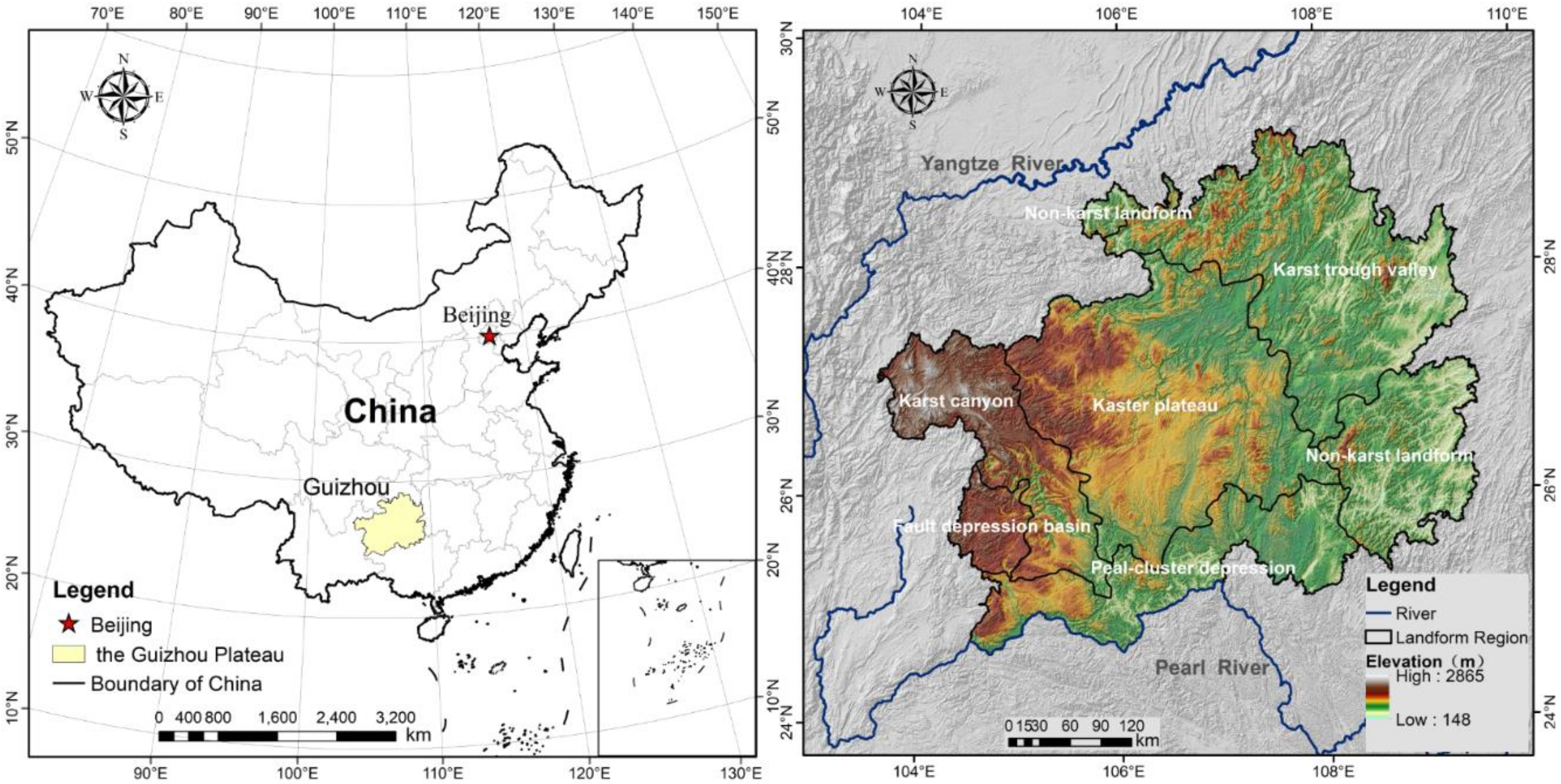
2.1. Study Area

The Guizhou Plateau is in southern China (24°37′–29°13′N, 103°36′–109°35′E). It has high elevation in the west and low elevation in the east (average elevation: 1100 m), and the landforms are predominantly typical karst-type landforms. According to the “Techniques standard for comprehensive control of soil erosion and water loss in karst region” (SL 461-2009) [42] and related studies [43,44], based on landform type and soil erosion, the study area can be divided into six landform regions: karst canyon, peak-cluster depression, fault depression basin, karst plateau, karst trough valley, and non-karst landform (Figure 1). The Guizhou Plateau has various soil types, and the zonal soil that includes red soil, yellow soil, and yellow-brown soil, accounts for 60.29% of the total area. Vegetation coverage on the Guizhou Plateau is high and the range of vegetation types diverse. The zonal vegetation is subtropical evergreen broadleaved forest. The area has a subtropical humid monsoon climate with little temperature change. The annual average temperature is in the range of 5–22 °C, and the annual average precipitation is in the range of 687–1657 mm. Owing to the characteristics of the landforms, soil types, climate, and hydrology, the Guizhou Plateau is highly susceptible to soil and water losses.
With the objective of improving the ecological environment, the Chinese government has implemented a series of ecological engineering projects in the Guizhou Plateau region. By 2015, the main ecological engineering projects within the region comprised the Natural Forest Protection Project (NFPP), Wildlife Conservation Nature Reserve (WCNR), Key Public Welfare Forest Project (KPWFP), Shelterbelt Forest Project (SFP), CCPRD, GGP, and some other forestry projects (OFP). The combined areas (39,700 km2) of these projects, of which the largest two are the NFPP followed by the GGP, account for approximately 22.56% of the total area of the plateau.

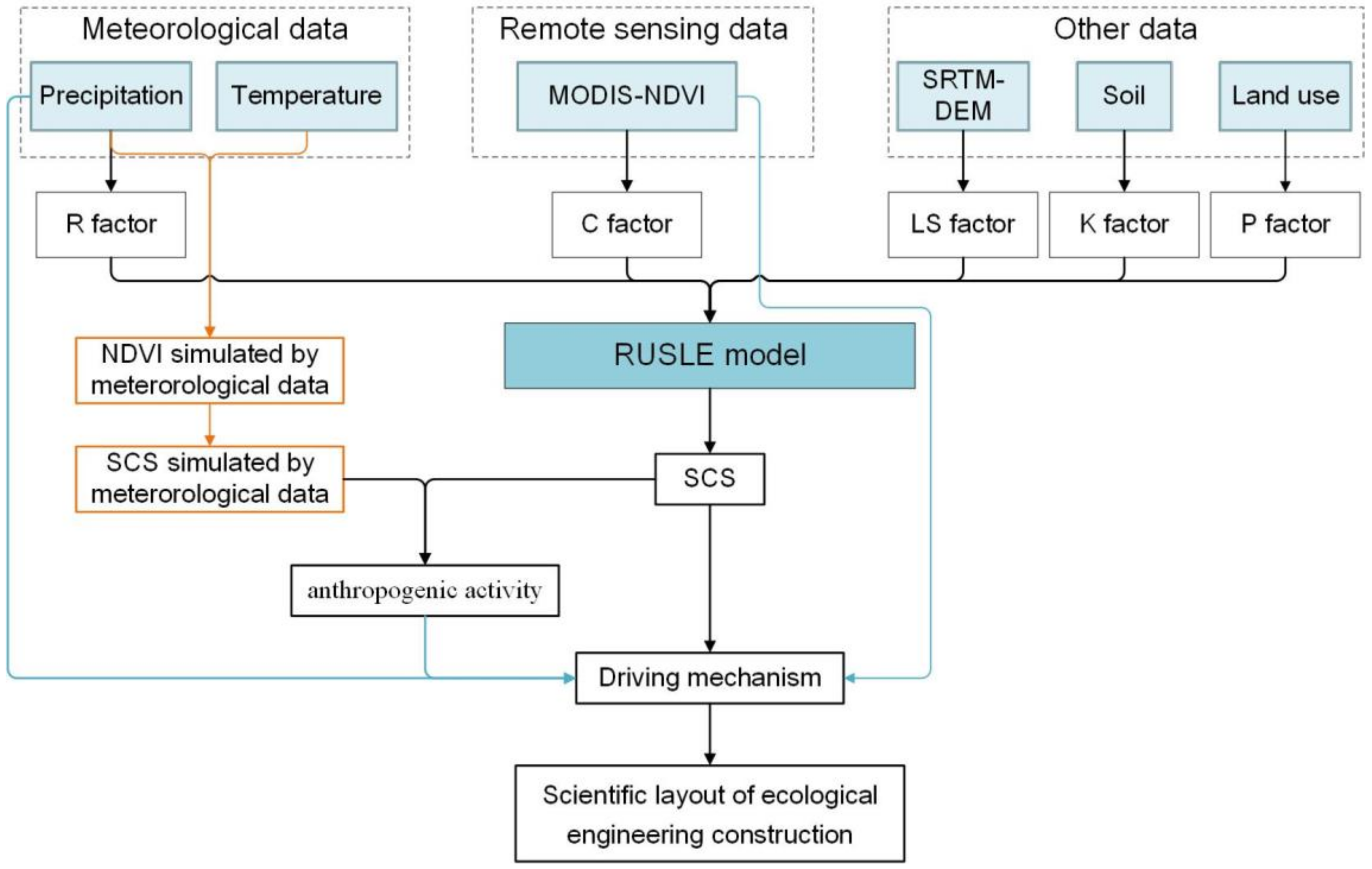
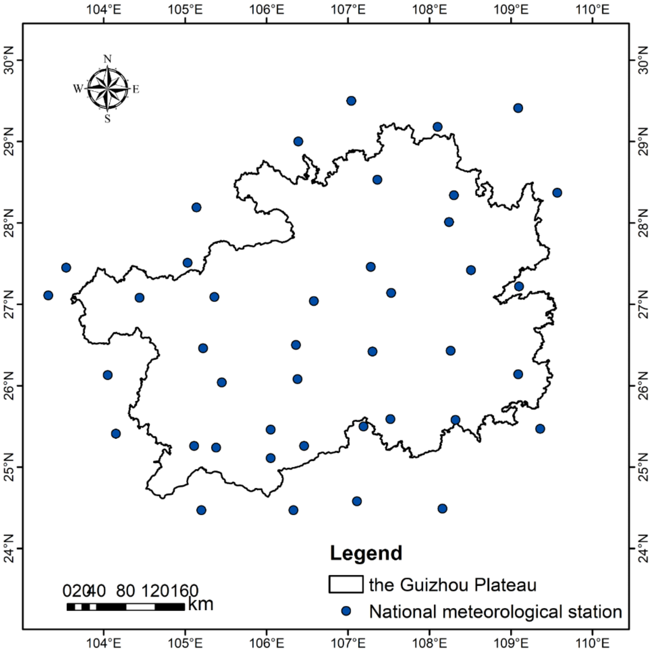
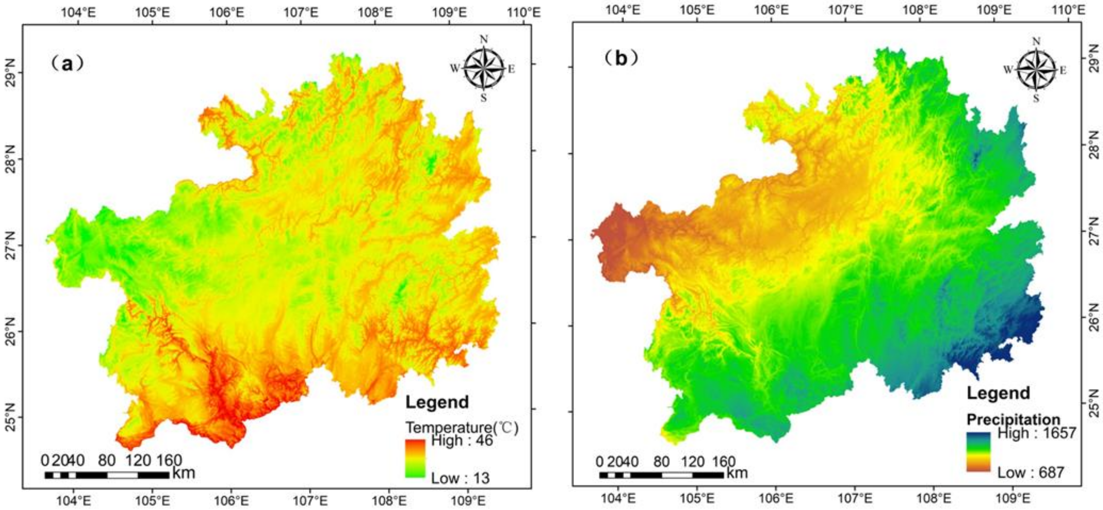
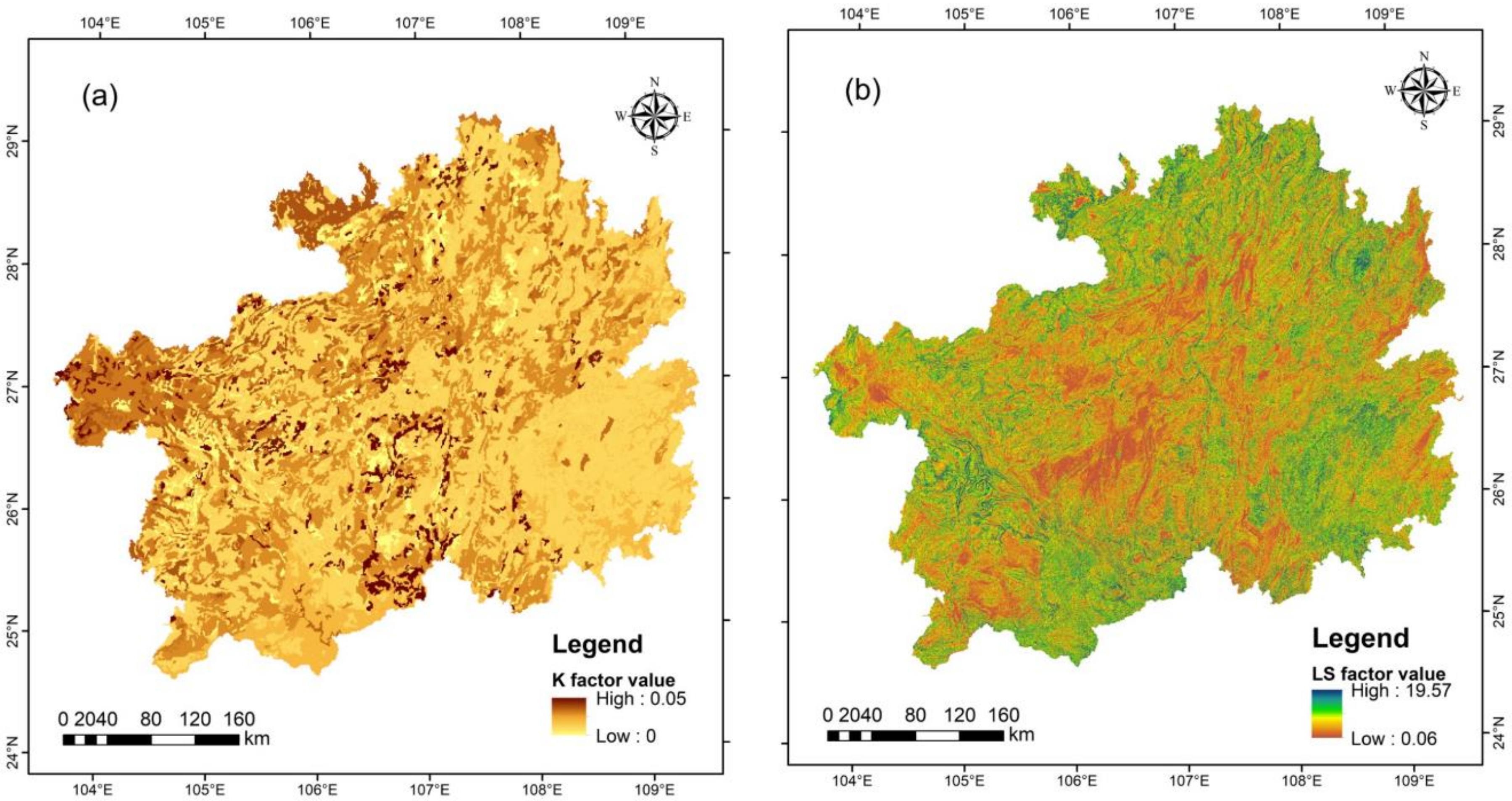
2.2. Data and Processing
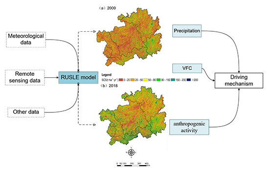
This study used meteorological data and RS data to evaluate SCS. The main methodological workflow is shown in Figure 2.
The meteorological data used in this study included precipitation, temperature, and other meteorological variables (1990–2018) recorded at 40 national meteorological stations located in the study area and within the surrounding 150 km (Figure 3). The dataset was obtained from the National Meteorological Information Center of China [45].
The ANUSPLIN professional meteorological interpolation software package, which is designed to target climate data, was used to interpolate the temperature and precipitation data. Although GIS software includes multiple spatial interpolation methods, ANUSPLIN specifically considers the accuracy, convenience, and time series length of the data and it has the advantage of being based on the theory of the thin plate spline function that produces high interpolation accuracy [46]. We used longitude and latitude which projected into the Krasovsky−1940 coordinate system as independent variables with which to interpolate precipitation to a spatial interpolation resolution of 250 m. The interpolated air temperature and precipitation raster data passed the generalized cross-validation procedure and the verification accuracy met the data analysis requirements. For consistency with the spatial resolution of the RS data, we processed both the precipitation and the temperature data to 250-m resolution to match the other datasets used in this study (Figure 4).
Soil data, based on the basic mapping unit for soil classes, were obtained from the China Soil Database [47], which included 12 soil classes, 61 soil types, and 227 soil subtypes. The attributes of soil sand content, soil clay content, soil silt content, and soil organic carbon content were used in the RUSLE model calculation.
The Digital Elevation Database of the Shuttle Radar Topography Mission (SRTM3) v4.1 was used to derive topographic data with 90-m resolution. These data were provided by the Geospatial Data Cloud site of the Computer Network Information Center (Chinese Academy of Sciences) [48]. The SRTM terrain data were obtained by the International Center for Tropical Agriculture using a new interpolation algorithm. SRTM terrain data can be divided into SRTM1 and SRTM3 datasets that have a corresponding resolution accuracy of 30 and 90 m, respectively. Currently, the published data have 90-m resolution (SRTM3), and these data were used in this study to calculate both the slope length and the slope of the terrain using an algorithm based on Zhang et al. [49].
The vegetation data used in this study comprised NDVI data for 2000–2018 derived from the MODIS NDVI dataset, which has 16-d temporal resolution and 250-m spatial resolution. We cropped the NDVI data according to match the study area and removed invalid fill values. The Maximum Value Composites method was used to extract the maximum value of the two mid-month NDVI values as the monthly NDVI value. This method, which can eliminate some of the effects of the atmosphere, satellite orbit drift, and other disturbances, has been proven to produce reasonable results for mountainous areas with complex terrain [39]. Then, the average of the monthly NDVI values is taken as the annual NDVI value. This method, which can characterize the annual average vegetation cover of an area, can be used to produce basic data for research and analysis. The spatial and temporal resolutions of these data are suitable for regional-scale analysis of the Guizhou Plateau. The VFC data were calculated using ENVI software based on the pixel dichotomy model. The pixel dichotomy method has been used in many studies to construct a model for vegetation coverage extraction based on satellite RS technology in combination with multispectral vegetation indices [50].
Land use data were derived from the China Land Use/Cover Dataset of 2000–2015 that includes 6 land grades and 25 land classes such as cultivated land, forest, grassland, construction land, and unused land. This dataset, which was created by Liu et al. [51], was obtained through considerable human–computer interactive interpretation based on China’s land use classification system and Landsat RS satellite data; the comprehensive evaluation accuracy is >94%.
Details of the area of ecological engineering and other related forest data related to the study area were obtained from the Fourth Survey of Forest Resources Planning and Design in Guizhou Province, provided by the Department of Forestry of Guizhou Province. These data, which cover the entire plateau, comprise 3,225,627 class records that include more than 100 property fields such as land use, altitude, slope direction, slope position, engineering category, type of land degradation, and desertification type. We mainly used the vector format of the boundary of ecological engineering areas for zonal statistics. The types and sources of the data used in this study are shown in Table 1. The main software to process these data was ArcGIS.

2.3. Methods

2.3.1. Soil Conservation Service Simulation

In this study, the SCS capacity was evaluated based on the soil erosion modulus. We used the SCS per unit area of soil conservation amount [52] to evaluate the SCS capacity in the study area. In this study, SCS was estimated using the RUSLE model [53]. The SCS represents the difference between the potential soil erosion under no vegetation cover and the actual soil erosion under the pertaining land use or land cover (Equations (1)–(3)).
Potential Soil Erosion :   A P = R × K × L S ,
Actual Soil Erosion :   A a = R × K × L S × C × P ,
SCS : A c = A p A a ,
where Ap is the potential soil erosion modulus [t·ha−1·yr−1], Aa is the actual soil erosion modulus [t·ha−1·yr−1], Ac is the SCS [t·ha−1·yr−1], R is the rainfall erosivity factor [MJ·mm·ha−1·h−1·yr−1], K is the soil erodibility factor [t·h·MJ−1·mm−1], LS is the slope length and slope steepness factor [dimensionless], C is the vegetation cover factor (dimensionless), and P is the soil and water conservation measure factor (dimensionless). All factors were calculated using ArcGIS and processed into 250-m-resolution raster data.
(1) Rainfall erosivity factor (R)
The rainfall erosivity factor is used to indicate the magnitude of rainfall erosivity. It is difficult to obtain data of rainfall energy and rainfall intensity; however, Wang et al. [54] found that the ratio of the sum of the squares of monthly precipitation and yearly precipitation had good correlation with R in karst areas. Hence, we used the model of Arnoldus et al. [55] (Equation (4)) to simulate rainfall erosivity in our study area:
R = i = 1 12 1.735 × 10 1.5 log P i 2 P 0.8188
where R is the rainfall erosivity factor [MJ·mm·ha−1·h−1·yr−1], Pi is the monthly rainfall [mm] (i = 1, 2, 3, …, 12), and P is the annual rainfall.
(2) Soil erodibility factor (K)
The soil erodibility factor can indicate the sensitivity of soil properties to erosion. In this study, we adopted the erosion-productivity impact calculator model of Williams et al. [56] (Equation (5)), and then we revised the soil erodibility calculated using this method following the study of Zhang et al. [57] (Equation (6)):
K E P I C = 0.2 + 0.3 exp 0.025 S A N 1 S I L 100 × S I L C L A + S I L 0.3 × 1.0 0.25 C C + exp 3.72 2.95 C × 1.0 0.7 S N I S N I + exp 5.51 + 22.9 S N I
K = 0.0183 + 0.51575 K E P I C × 0.1317
where K is the revised soil erodibility factor, SAN is the content of soil sand (particle size: 0.1–2.0 mm, %), SIL is the content of soil silt (particle size: 0.002–0.1 mm, %), CLA is the content of soil clay (particle size < 0.002 mm, %), C is the content of soil organic carbon (%), and SNI = 1 − SAN/100.
(3) Topographical factor (LS)
The topographical factor, which is the combination of the two factors of slope length and slope steepness, represents the influence of topography on soil loss. In this study, the calculation method proposed by Wischmeier et al. [30] and McCool et al. [34] was used to calculate the topographical factor (Equations (7)–(10)):
L = γ 22.13 α
α = β β + 1
β = sin θ / 0.0896 3.0 × sin θ 0.8 + 0.56
S = 10.8 × sin θ + 0.03 θ < 5 % 16.8 × sin θ 0.50 5 % θ 10 % 21.91 × sin θ 0.96 θ > 10 %
where L is the slope length factor, S is the slope factor, γ is the slope length (m), θ is the slope (%), α is the variable slope length index, and β is the coefficient that varies with slope.
(4) Vegetation cover factor (C)
This factor is directly related to vegetation coverage and its value is in the range of 0–1. In this study, we adopted the method for the calculation of the vegetation cover factor proposed by Cai [58] (Equations (11) and (12)):
C = 1 V F C = 0 0.6508 - 0.3436 lg f 0 < V F C 78.3 % 0 V F C > 78.3 %
V F C = N D V I N D V I s o i l N D V I max N D V I s o i l
where NDVIsoil is the NDVI value of bare soil pixels and NDVImax is the NDVI value of pure vegetation pixels. Based on the obtained vegetation index, we took the confidence intervals of NDVI of 5% and 95% as pure bare soil pixels and pure vegetation pixels, respectively, and we replaced NDVI values lower (higher) than the pure bare soil (vegetation) pixel value with the minimum (maximum) value.
(5) Soil and water conservation measure factor (P)
The soil and water conservation measure factor (P) refers to the ratio of the soil loss after adopting certain soil and water conservation measures to the soil loss without taking any measures. Following a study in Guizhou Province by Wang et al. [59], we assigned certain values to different land use types (Table 2).

2.3.2. Correlational Analyses

Correlation analysis is a statistical method for studying the correlation between two or more variables. We established a linear regression model to fit the multiyear trends (2000–2018) of precipitation, vegetation coverage, and SCS, respectively. The degree of correlation between pairs of variables was represented by the Pearson correlation coefficient [60], and the significance level was expressed by the t-test statistic (Equations (13) and (14)):
R = i = 1 n X i X ¯ Y i Y ¯ i = 1 n X i X ¯ 2 i = 1 n Y i Y ¯ 2
t = R n 2 1 R 2
where R is the Pearson correlation coefficient, X and Y are the two variables, X ¯ and Y ¯ are the averages of the two variables, respectively, and i is the i-th year. With the calculated t-test statistic, the corresponding p-value was used to determine the significance level between the variables. In this study, the NDVI, annual rainfall, and SCS on the Guizhou Plateau during 2000–2018 were selected as variables for the correlation analysis, which was programmed using the MATLAB package.

2.3.3. Residual Analysis

In this study, we considered that ecological engineering would change the vegetation coverage. Therefore, residual analysis was used to eliminate the climatic factors of temperature and precipitation in the long-term time series variation of the NDVI. As a series of large-scale ecological engineering projects commenced in 2004, we chose 2004 as the time node. The NDVI, temperature, and precipitation during 2000–2004 were introduced into the regression model to establish a per-pixel NDVI–climate regression model. Then, temperature and precipitation data for 2000–2018 were inserted into the model to obtain predicted NDVI values under the prevailing meteorological conditions without the implementation of ecological engineering projects [39] (Equation (15)):
N D V I ( i , t ) = a T ( i , t ) + b P ( i , t ) + c
where NDVI(i,t), T(i,t), and P(i,t) represent the NDVI value, temperature, and precipitation of the i-th pixel in the t-th year, respectively; a and b are the regression coefficients of NDVI(i,t) to T(i,t) and P(i,t), respectively; and c is a constant.
The SCS, NDVI, and precipitation for 2000–2004 were introduced into the regression model to establish a per-pixel SCS regression model. Then, the predicted values of the NDVI and precipitation for 2000–2018 were inserted into the model to obtain the predicted values of SCS under the prevailing meteorological conditions without the implementation of ecological engineering projects (Equation (16)):
S C S ( i , t ) = a N D V I ( i , t ) + b P ( i , t ) + c
where SCS(i,t), NDVI(i,t), and P(i,t) are the SCS, temperature, and precipitation of the i-th pixel in the t-th year, respectively; a and b are the regression coefficients of SCS(i,t) to NDVI(i,t) and P(i,t), respectively; and c is a constant.
The predicted SCS under the prevailing meteorological conditions without the implementation of ecological engineering projects was obtained based on the above two formulas. The actual SCS obtained using the RUSLE model was subtracted from the predicted value to obtain the residual sequence representing the effect of anthropogenic activities [61]:
ε ( i , t ) = S C S r e a l ( i , t ) S C S p r e d i c t ( i , t )
where ε (i,t), SCSreal(i,t), and SCSpredict(i,t) represent the residual sequence of anthropogenic activities [t·ha−1·yr−1], the SCS calculated using the RUSLE model [t·ha−1·yr−1], and the predicted SCS [t·ha−1·yr−1], respectively. A value of ε of >0 (<0) was considered to reflect a positive (negative) effect of ecological engineering on SCS; a value of ε ≈ 0 was considered to reflect weak effect. The spatial distribution of the intensity of the effect of ecological engineering projects on SCS was obtained based on the average value of the residual sequence of 2000–2018, following which the Mann–Kendall test was used to determine the significance of the trend. The z value of the statistic is a standard normal distribution, generally taken as α = 0.05; when |z| > 1. 96, the confidence level of the study sequence α is <0.05, and when |z| < 1.96, the confidence level α is >0.05 [62]. The Mann–Kendall test [63] was used to determine the temporal trend of the residual sequence value and to obtain the significant distribution of the change of the SCS function under the influence of ecological engineering; thus, making the results more credible scientifically.

3. Results

3.1. Spatial and Temporal Characteristics of SCS

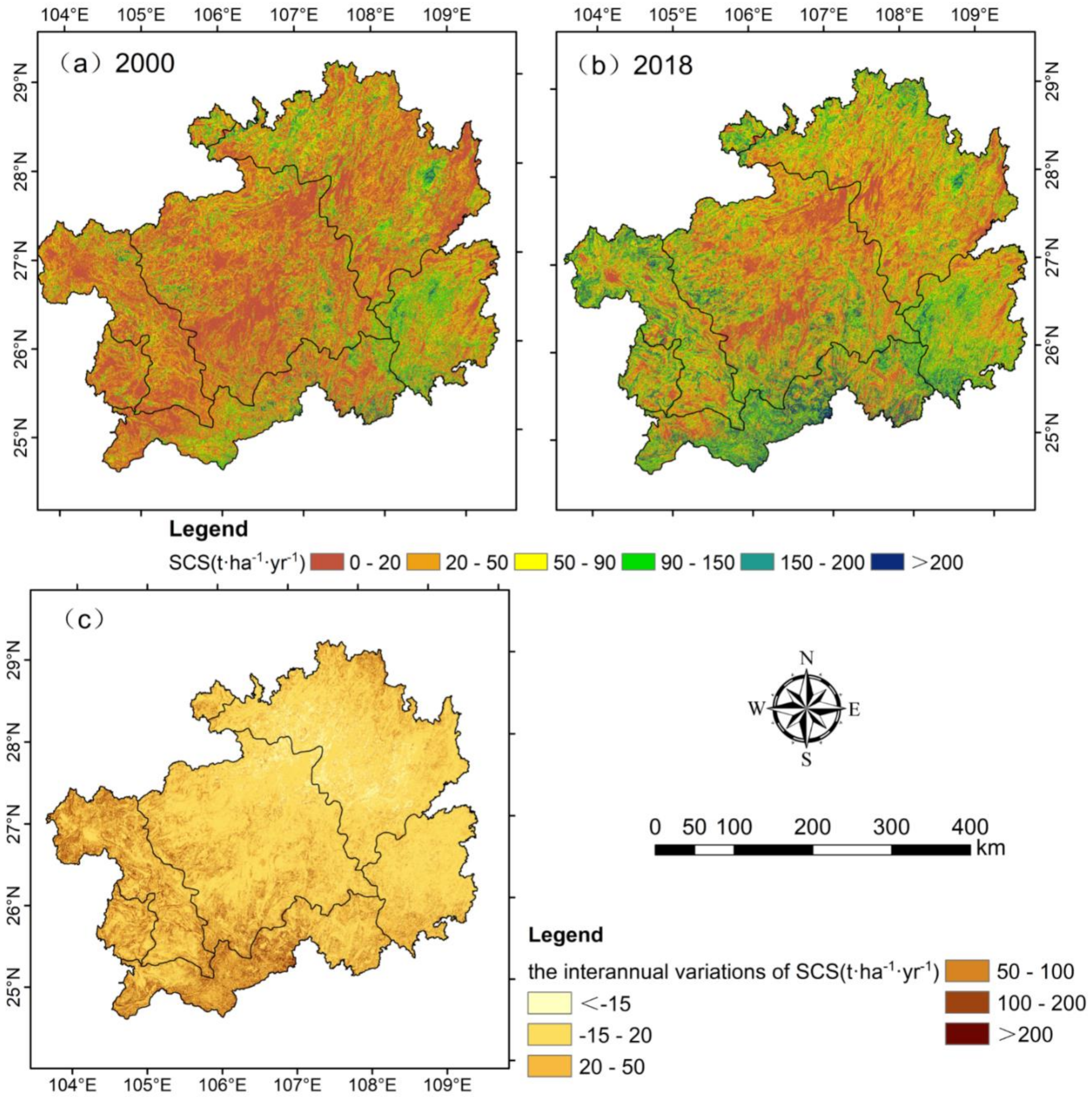
3.1.1. Spatiotemporal Variation of SCS

The R, K, LS, C, and P factors used in the RUSLE model were simulated using GIS software. The R, C, and P factors change annually, whereas the K and LS factors are fixed (Figure 5). The average SCS on the Guizhou Plateau during 2000–2018 was 50.67 t ha−1 yr−1; the lowest (32.09 t·ha−1·yr−1) and highest (87.06 t·ha−1·yr−1) values occurred in 2013 and 2017, respectively. As shown in Figure 6, SCS on the Guizhou Plateau showed an overall upward trend during 2000–2018 at a rate of 1.39 t·ha−1·yr−1, significant at the p = 0.05 level, which indicates that the SCS function improved.
Regionally, based on the annual SCS, the area of the Guizhou Plateau with the strongest SCS was in the southeast, where non-karst landforms and peak-cluster depressions form the primary landform types. This area comprises a forest ecosystem with high vegetation coverage, low anthropogenic activity, and an excellent ecological environment. The areas with the weakest SCS function were in central and western parts of the Guizhou Plateau, characterized by karst canyons and karst plateaus with serious soil and water losses. Central parts of Guizhou Province are characterized by many cities with high levels of socioeconomic development and widespread anthropogenic activities. The areas of greatest SCS improvement (>50 t·ha−1·yr−1) within the study area were primarily in the southwest, whereas the regions with the greatest deterioration were mainly in the north (Figure 7).

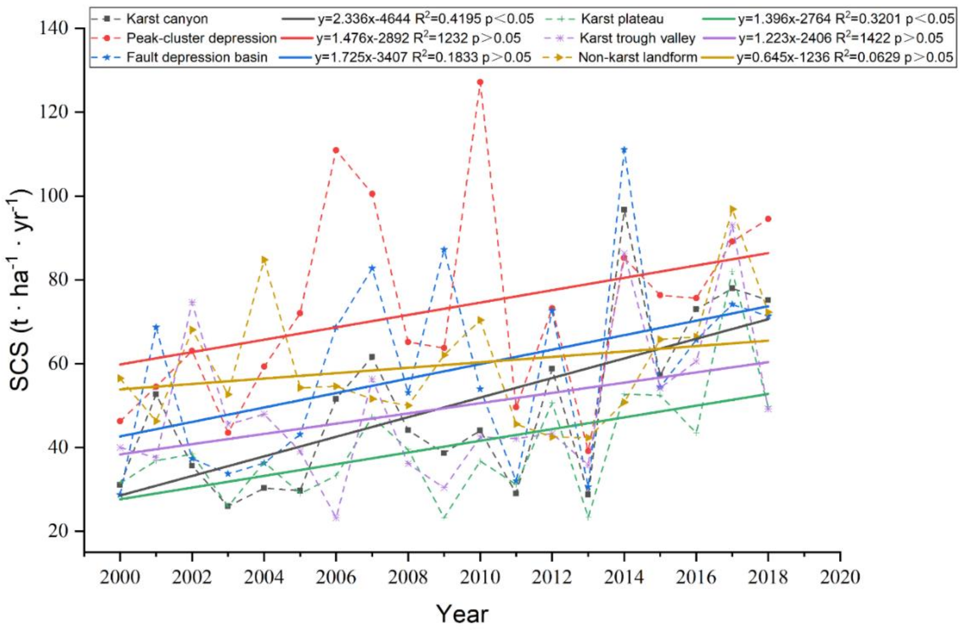
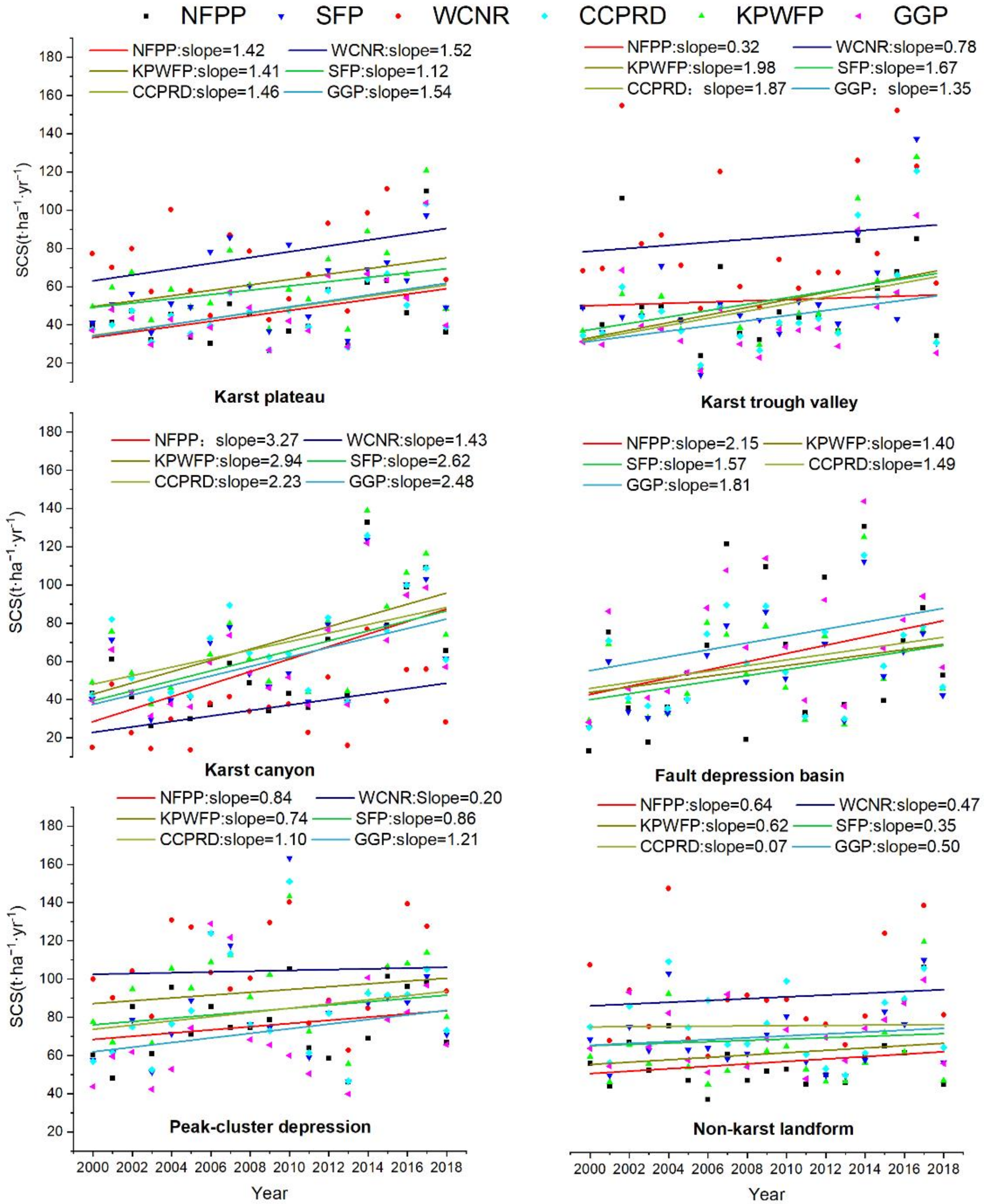
3.1.2. Spatiotemporal Variation of SCS in Different Landform Regions

In terms of landform region, the highest SCS was 73.12 t·ha−1·yr−1 in the peak-cluster depression region located in the south of the study area, followed by the non-karst landform regions (59.69 t·ha−1·yr−1); the lowest SCS (40.22 t·ha−1·yr−1) was in the central karst plateau region (Table 3). The SCS of all landform regions showed an upward trend; the most rapid improvement (2.34 t·ha−1·yr−1) was in the karst canyon region and the slowest rate of improvement (0.65 t·ha−1·yr−1) was in the non-karst landform regions. The karst canyon and fault depression basin regions in the high-elevation area of the western Guizhou Plateau have long had fragile ecological environments with serious soil and water losses. Conversely, the non-karst region in the east of the study area has lower elevation, relatively flat terrain, and high forest coverage, and its historical ecological background is better than that of the other landform regions (Figure 8).
Among the different landform regions, comparison of the 2000 and 2018 data reveals that the geomorphic areas in which SCS has increased included the karst canyon, fault depression basin, and peak-cluster depression regions. Conversely, SCS has reduced in the non-karst landform and karst trough valley regions and remained largely stable in the karst plateau region. In terms of the total amount, the same conclusion can be reached (Figure 9), i.e., the SCS capacity of most karst areas increased, whereas that of non-karst areas declined.

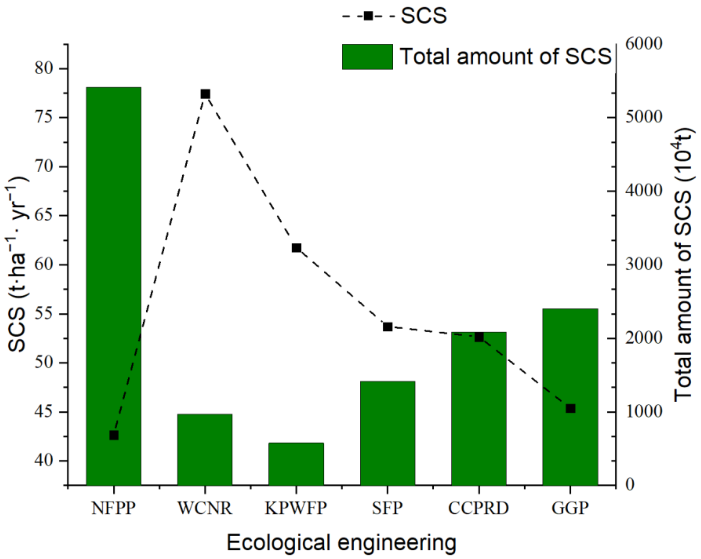
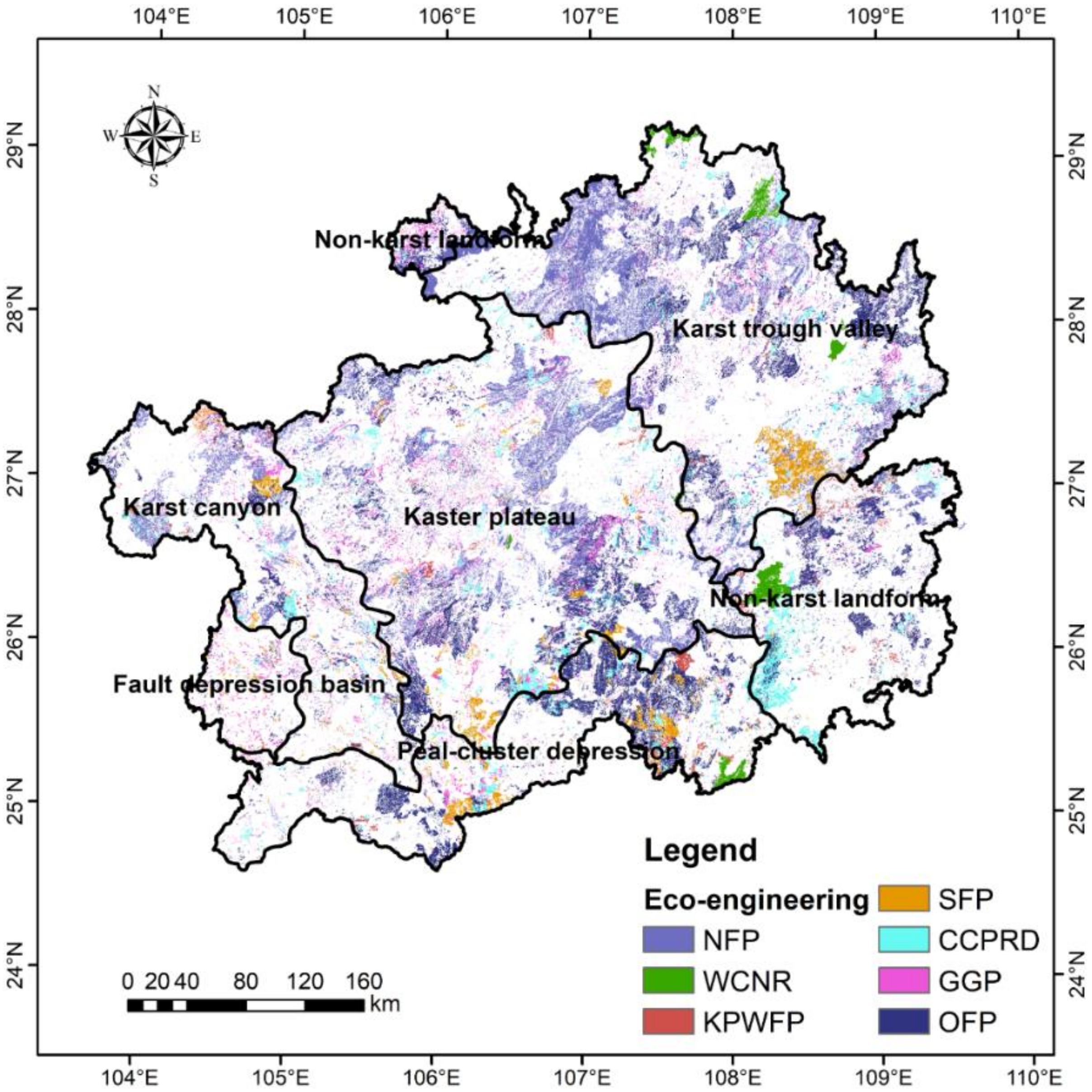
3.1.3. Spatiotemporal Variation of SCS in Different Ecological Engineering Areas

In the different ecological engineering areas, the highest proportion of the total area is associated with the NFPP (7.20%), followed by the GGP (3.01%); the smallest area is associated with the KPWFP. Among the different ecological engineering areas, the WCNR has the highest SCS (77.44 t·ha−1·yr−1) and its implementation area accounts for 0.71% of the total area. The NFPP has the lowest SCS (42.66 t·ha−1·yr−1) and its implementation area accounts for 7.2% of the total (Table 4). The SCS of the WCNR is much higher than that of the other ecological engineering areas. The project area is focused primarily on the nature reserve, which has a reasonable ecological environment and abundant vegetation layers; however, there are few nature reserves on the Guizhou Plateau. The NFPP has the highest total amount of SCS (much higher than other ecological engineering projects) and its area of implementation is largest, followed by the GGP (Figure 10).
The SCS of the different ecological engineering projects in the different landform regions (2000–2018) was analyzed; however, there was no WCNR in the fault depression basin region. The NFPP, KPWFP, SFP, CCPRD, and GGP in the karst canyon region all showed the highest upward trend of SCS: 3.27, 2.94, 2.62, 2.23, and 2.48 t·ha−1·yr−1, respectively. The SCS of the WCNR improved rapidly in the karst plateau region, which is a major landform of the Guizhou Plateau, characterized by plain terrain and deep soil layers that make it a suitable habitat for the survival of wildlife. The CCPRD improved the SCS function considerably in the various karst landform areas. This reflects the various control measures implemented to improve the damaged natural ecosystem in areas of rocky desertification, areas, which have had obvious effect on the improvement of soil and water conservation in karst areas. The SCS of each ecological engineering area improved slowly in non-karst landform areas. Overall, the construction of ecological engineering projects has had marked effect on SCS in karst landform areas but not so in non-karst landform areas (Figure 11).

3.2. Analysis of Driving Mechanism of SCS

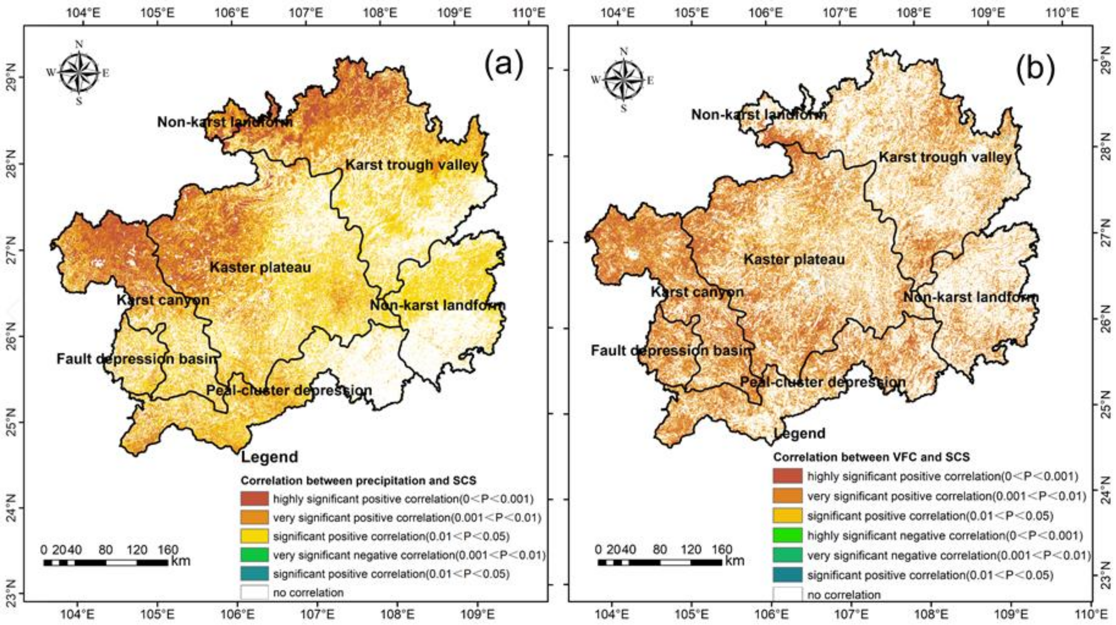
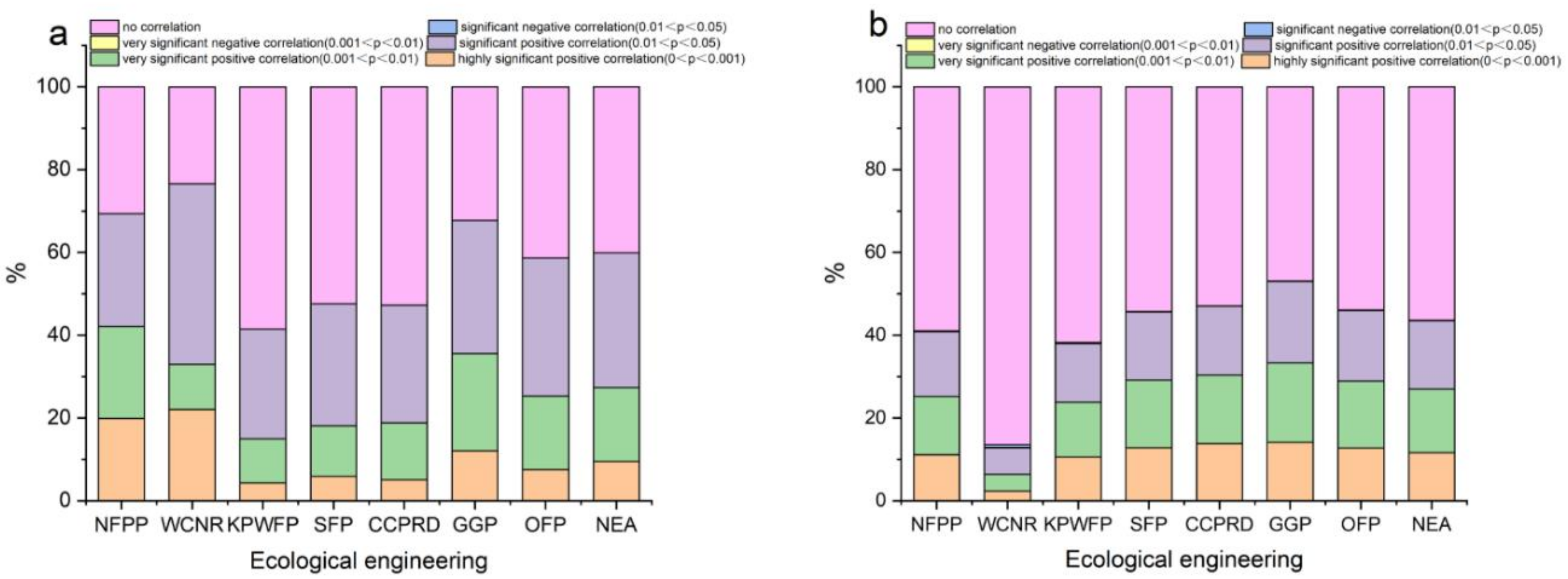
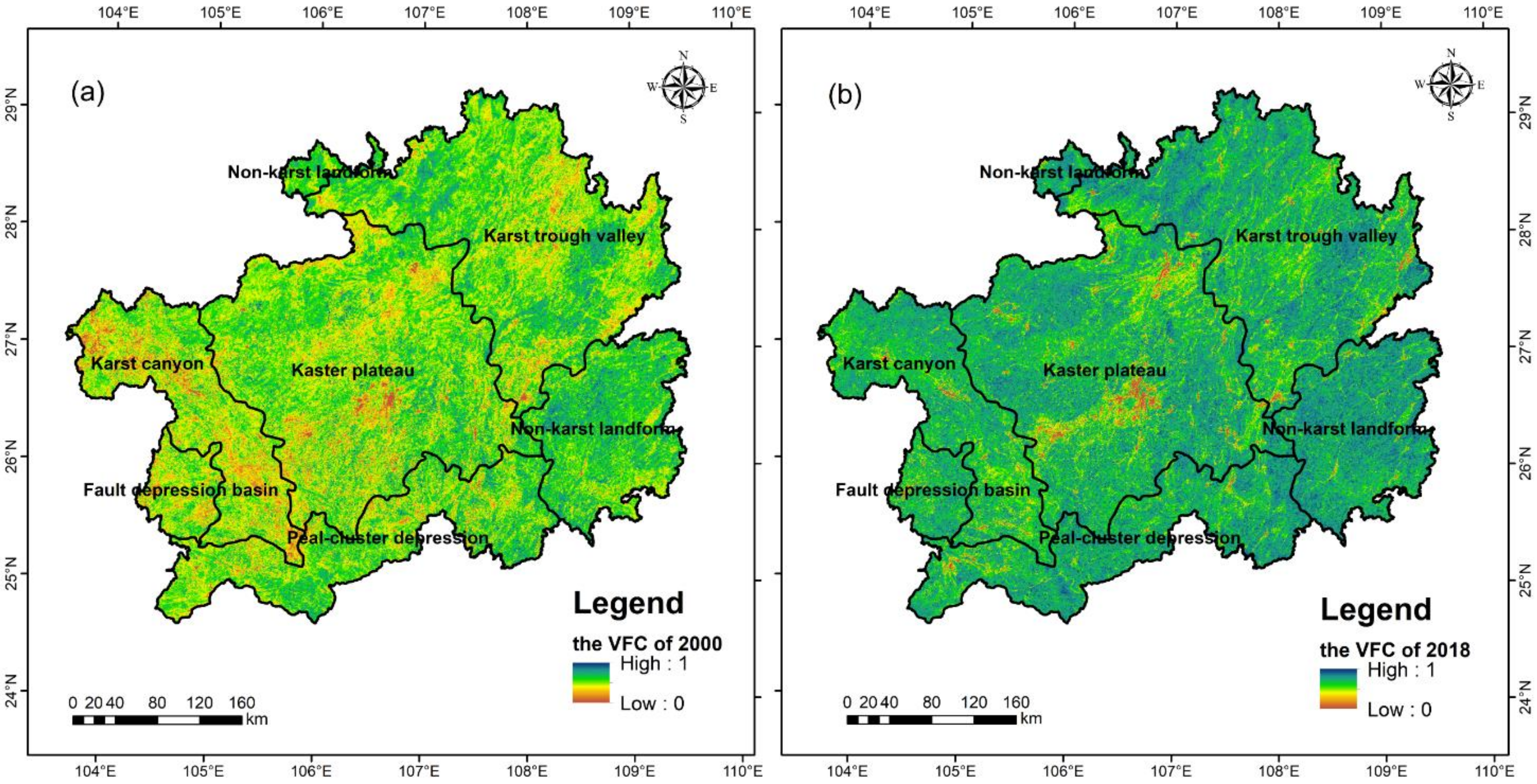
3.2.1. Driving Effect of Precipitation and VFC on SCS

SCS is affected by various factors that can be divided into natural factors and anthropogenic activities. Among the former, precipitation and VFC are the most important factors affecting soil erosion [64]. The Pearson method was used to calculate the degree of correlation of both precipitation and VFC with SCS during 2000–2018, and the t-test statistic was calculated to assess the significance of the results.
During 2000–2018, areas with significant positive correlation between the annual variations of precipitation and SCS, which accounted for 59.43% of the total area, were located in northern and northwestern parts of the Guizhou Plateau (p < 0.05) (Figure 12a). In addition, areas in which VFC also had significant positive correlation with SCS (accounting for 47.26% of the total area) were distributed widely throughout the entire study area, but concentrated primarily in western parts (p < 0.05) (Figure 12b). Neither precipitation nor VFC showed significant negative correlation with SCS on the Guizhou Plateau. Areas of significant positive correlation of SCS with precipitation were mainly in northern parts of the karst trough valley region as well as some parts of the karst canyon and karst plateau regions. Moreover, VFC mainly affected SCS in the southwest of the study area, which includes the karst canyon, fault depression basin, and peak-cluster depression regions.
In the different ecological engineering areas, there was only positive correlation between precipitation, VFC, and SCS. The highest proportion of positive correlation between precipitation and SCS was in association with the WCNR (76.59%) and the lowest was in association with the KPWFP (41.37%). For VFC, the GGP and the WCNR had the highest and lowest proportion of positive correlation with SCS, respectively, i.e., 53.02% and 12.81%, respectively (Figure 13). A probable explanation is that the WCNR is mainly a natural reserve with high vegetation coverage, in which excessive rainfall could lead to intensified potential soil erosion that might increase SCS. Moreover, the GGP directly converts large areas of cultivated land with severe soil erosion and rocky desertification into forest, restoring the vegetation, directly controlling soil erosion, and improving the SCS function. In each ecological engineering area, both precipitation and VFC were positively correlated or uncorrelated with SCS, i.e., neither exhibited any negative correlation.

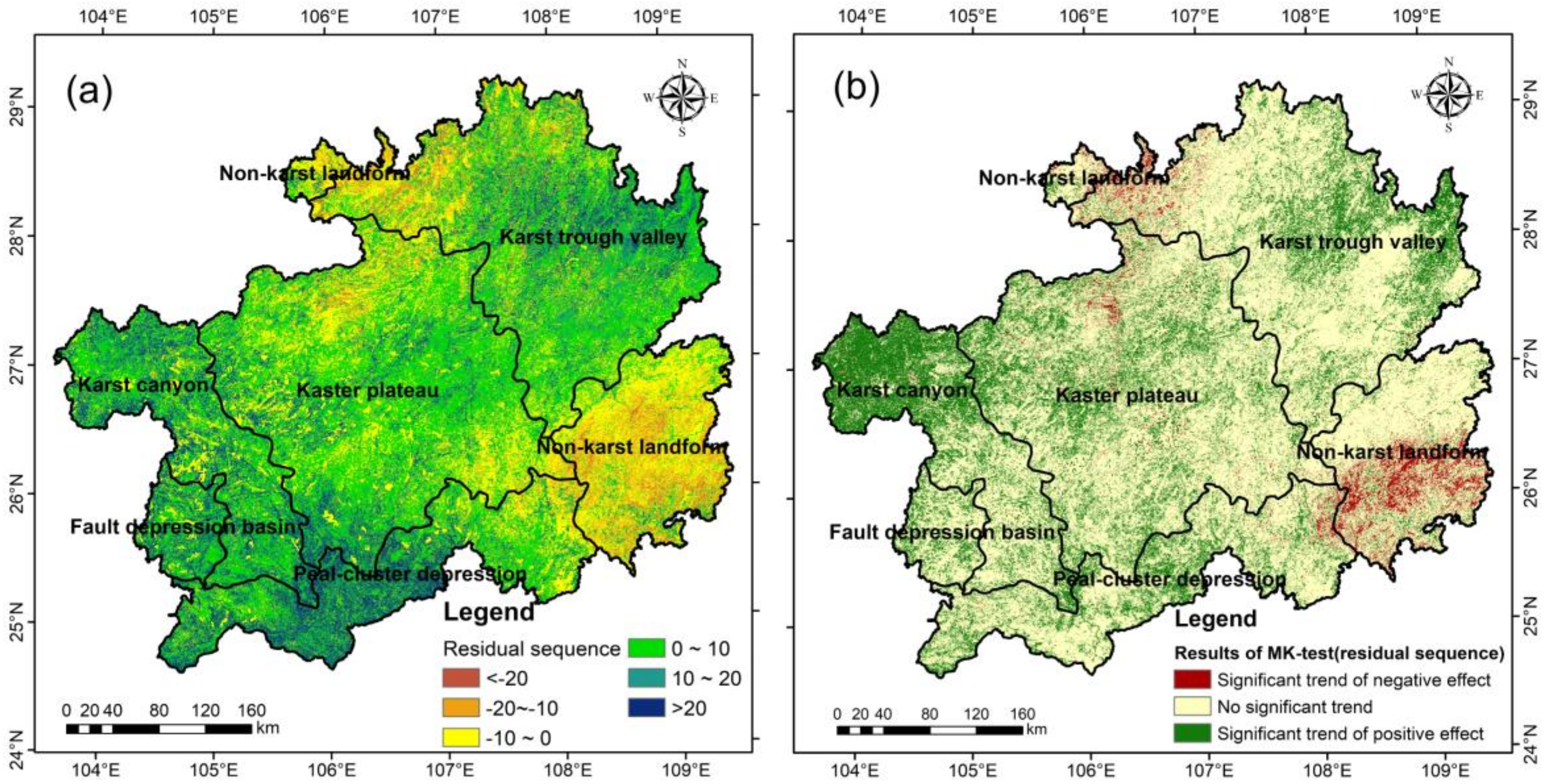
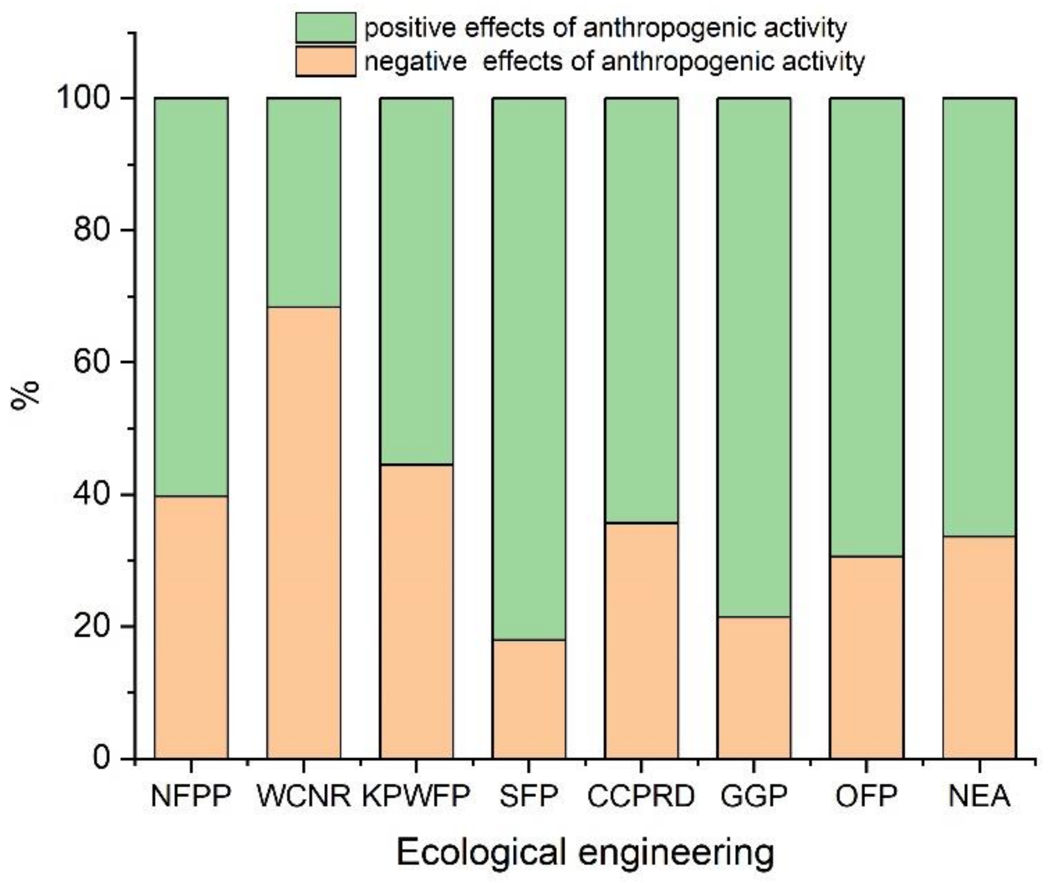
3.2.2. Driving Effect of Anthropogenic Activities on SCS

We predicted the NDVI based on temperature and precipitation data without the effect of ecological engineering implementation, and then used it to simulate the predicted value of SCS. This could exclude the impact of vegetation change caused by ecological engineering implementation. The effect of anthropogenic activities was obtained through residual sequence analysis. The average R2 of the modeled SCS was 0.61, and 16.1% of pixels passed the 0.05 significance level test. In addition, SCS predicted by the regression models and the real SCS exhibited high correlation (0.80) in terms of the spatial distribution, reaching significant correlation at the p < 0.05 level. Given that the time series used for the regression was short and that the study area has very complex terrain and climatic conditions, it was considered suitable for achieving the purposes of this study.
In this study, the average annual residual value of the study area was 5.71 during 2000–2018. According to the spatial distribution of the average annual residual value during 2000–2018 (Figure 14a), it can be seen that anthropogenic activities have had a primarily positive effect on SCS. The high-value regions of this positive effect were located in northeastern and western parts of the study area, i.e., primarily in karst trough valley, karst canyon, fault depression basin, and peak-cluster depression regions. Conversely, the areas of negative effect were distributed mostly in southeastern and northern parts of the study area, i.e., mainly non-karst landform regions. According to the Mann–Kendall significance trend test (Figure 14b), the areas in which the trend of the effect of anthropogenic activities was significantly positive (negative) accounted for 26.43% (3.97%) of the entire study area (p < 0.05). Overall, the positive effect of anthropogenic activities on SCS has been stronger than the negative effect. It can be concluded that anthropogenic activities such as ecological engineering construction have had positive effects in karst landform areas and negative effects in non-karst landform areas.
The distribution of ecological engineering projects in the study area (Figure 15) shows that the NFP is distributed widely in various ecological engineering areas, the GGP is distributed mainly in karst landform areas, and the WCNR is distributed primarily in non-karst landform areas. It can be seen from the spatial distribution of ecological engineering areas that the areas in which the effect of anthropogenic activity is positive (i.e., where the residual sequence is >0) were generally distributed in areas in which ecological engineering projects are implemented, especially in the karst landform regions. Conversely, in non-karst landform regions, even if certain ecological engineering projects were implemented (e.g., the WCNR), the effect of anthropogenic activities was negative, whereas in areas without implementation of ecological engineering projects, the effect of anthropogenic activities had a significant negative trend. It can be concluded that particular attention should be paid to soil and water losses as well as to the implementation of ecological engineering projects in non-karst landform regions.
The average residuals of the different ecological engineering projects during 2000–2018 are listed in Table 5. The SFP has the highest value (10.21) because this ecological engineering project has the greatest positive effect on the SCS function. The WCNR is the only ecological engineering project to have a negative residual value (−3.11). It can be concluded that ecological engineering construction has generally had positive effect on the SCS function, although certain anthropogenic activities in the WCNR could have had negative impact on the ecosystem that might have led to soil and water losses.
For the different ecological engineering projects, the areas of positive and negative effects of anthropogenic activities have different proportions. The ecological engineering project with the highest proportion of positive effects associated with anthropogenic activities is the SFP (82.06%). Moreover, the areas with positive effects associated with anthropogenic activities accounted for >60% of the total area for the GGP, CCPRD, and NFPP. Conversely, the area of the WCNR that exhibited negative effects associated with anthropogenic activities accounted for 68.44% of the total area. The WCNR was the only ecological engineering project to have a negative area that accounted for >50% of its total area (Figure 16).
Comparison of the change in VFC during 2000–2018 reveals that vegetation has generally improved, especially in karst canyon, fault depression basin, and karst trough valley regions (Figure 17). In considering the impact of anthropogenic activities on SCS, the most important factor is the coupling relationship between vegetation change and anthropogenic activity. Ecological engineering construction changes the vegetation coverage and affects SCS indirectly. Following the implementation of the various ecological engineering projects in the study area, vegetation coverage increased considerably in all karst landform regions, e.g., the VFC in the karst canyon region was 0.72 in 2000 and 0.80 in 2018 (Table 6). Conversely, vegetation coverage increased only slightly in the non-karst landform regions (0.81 in 2000; 0.84 in 2018). In addition, it is evident that VFC increased markedly following the implementation of all the ecological engineering projects except the WCNR. The VFC associated with the GGP was 0.76 in 2000 and 0.84 in 2018, which indicates that the implementation of GGP is more appropriate in specific areas. In contrast, VFC in the WCNR was 0.84 in 2000 and 0.83 in 2018, i.e., a slight reduction.

4. Discussion

4.1. Model Simulations of Soil Erosion Modules and SCS

In this study, the R, K, LS, C, and P factors used in the RUSLE model were simulated using local rainfall data, RS data, and regional ecological engineering data. All factors were processed into raster data with 250-m resolution and used to simulate the soil erosion modulus as well as SCS through parameter localization. The simulation of the R factor in this study was based on interpolation of rainfall data using ANUSPLIN (spatial resolution: 250 m). According to Yue et al. [65], the average absolute error of the interpolation results in each grid is changed only slightly when the size of the grid is increased from 50 to 1000 m. This is mainly related to the scale of the spatial distribution of rainfall, which usually varies little within the range of 1 km2. The factor values of L and S obtained from DEMs with different spatial resolution are notably different [66], Generally, topography tends to be flattened in small-scale DEM data and the slope decreased, which means the intensity of soil erosion could be underestimated [67], whereas the slope value of a real surface cannot be reflected directly by large-scale DEM data [68]. Given the difficulty in obtaining high-resolution DEM data and recognizing the complex topography of our study area, we chose 90-m resolution DEM data. Such data, which are considered suitable for large-scale spatial analysis, made the calculation of the topographical factor more accurate and were appropriate for the karst landform and terrain fragmentation in the study area. The value of the P factor reflects the characteristics of different soils and water conservation measures, e.g., crop rotation, ground cover, and contour tillage. Generally, values of the P factor are obtained based on RS imagery and assigned according to land use type on the large scale [69]. We used land use data of 2000–2015 to assign the values of the P factor, which could well reflect the impact of land use and land cover changes on soil erosion. The original 1-km resolution data were changed to 250-m resolution by resampling because of the difficulty associated with obtaining high-resolution land use data. To improve the accuracy of the results, water bodies and construction land were directly assigned a value of zero. Despite the many uncertainties involved in the acquisition and determination of the R, K, L, S, C, and P factors, and the difficulty in assessing their accuracy [68], we consider that the selected data had sufficient precision to ensure the validity of the final result.
During our study, the annual average actual soil erosion modulus on the Guizhou Plateau during 2000–2018 was 10.51 t·ha−1·yr−1, and the soil erosion modulus calculated using the RUSLE model in 2000 was 18.84 t·ha−1·yr−1. This is in reasonable agreement with the average annual soil modulus of the Proclamation of Soil and Water Loss in Guizhou Province in 2000 (14.32 t·ha−1·yr−1 issued by the Water Resources Department of Guizhou, China [70]. In addition, using the RUSLE model, both Gao et al. [71] and Zeng et al. [72] calculated the soil erosion modulus of certain areas of the Guizhou Plateau as 15.08 and 14.40 t·ha−1·yr−1, respectively. Thus, given this level of accord, we believe that our evaluation of SCS using the RUSLE model and the data described in Section 2.2 had satisfactory accuracy.
In this study, we used the RUSLE model to investigate the sensitivity of SCS on the annual timescale. However, soil erosion has strong seasonal variation owing to the influence of natural conditions [73]. Based on a study in Danjiangkou (China), Feng et al. [74] reported that soil erosion in summer and autumn was higher than in spring and winter, the main reason for which was the uneven distribution of rainfall throughout the year. The plant canopy is another important factor influencing soil and water conservation. Wu et al. [75] found that crops with marked seasonal changes of characteristics throughout the year had notable influence on soil loss on the Loess Plateau (China). If monthly scale data could be obtained, the relative impacts of vegetation and precipitation could be reflected more clearly.

4.2. Characteristics of SCS

In the Guizhou Plateau region, SCS has generally improved during 2000–2018 with an upward trend of 1.39 t·ha−1·yr−1. Analysis of the change of VFC during 2000–2018 revealed an upward trend of VFC in the Guizhou Plateau region. The average annual VFC during 2000–2004 (2014–2018) was 0.77 (0.82). Moreover, the average VFC was >0.8 in each year during 2014–2018. According to Gao et al. [71], when vegetation coverage is >0.5–0.6, soil erosion decreases with a further increase in vegetation coverage. It is widely believed that vegetation restoration could improve the SCS capacity substantially [76]. The findings of this study corroborate the results of previous related research. In Guizhou Province, the experimental work of the GGP and NFPP began in 2000. In 2001, the SFP, WCNR, and KPWFP were initiated in the Yangtze River Basin. Since 2004, large-scale implementation of the CCPRD has been undertaken, and various other ecological engineering projects have been performed. The ecological engineering measures such as the GGP have been shown to increase vegetation coverage and enhance the soil and water conservation capacity [77].
On the Guizhou Plateau, SCS was found to show high spatial heterogeneity. Geomorphology is known to affect the soil erosion rate [78]. Areas with high SCS were found mainly in southeastern parts of the Guizhou Plateau, i.e., in non-karst landform and peak-cluster depression regions. Areas with lower SCS were found primarily in central and western areas, i.e., the karst plateau and karst canyon regions. Comparison of non-karst landform and karst landform areas revealed that the underlying surface of the former is more suitable for vegetation growth [44] and more conducive to vegetation recovery. In contrast, the decline in the rate of soil erosion is faster in non-karst landform regions than in karst regions that have terrain fragmentation and a fragile ecological environment [72]. Moreover, the central karst plateau region is mainly an urban ecosystem with notable urban construction activities, high population density, and considerable anthropogenic interference [79]. In the western karst region of the Guizhou Plateau, soil erosion has a complex relationship with topography, lithology, and the degree of rocky desertification [80,81].
The areas with increased SCS were found mainly in the western karst canyon and the southern peak-cluster depression regions, of which the latter exhibit the most obvious improvement. In comparison with other areas of the Guizhou Plateau, the hydrothermal conditions of southern parts are more advantageous for vegetation growth and recovery [39]. Following the implementation of many ecological engineering projects, especially the GGP that has returned areas of steep farmland to forest, SCS on the Guizhou Plateau has improved significantly. The karst canyon region in the west of the study area has a history of intense tectonic activity that has led to widespread distribution of highly eroded carbonate rocks. The regional topography is complex and the ecological environment fragile [82]. Following the implementation of ecological engineering projects such as the KPWFP and NFPP in these areas, which expanded the area of forest to protect the existing vegetation, the SCS function was improved. However, improvement of the SCS function in non-karst landform regions was not obvious; in some cases, it actually exhibited a downward trend. Historically, the ecological background of non-karst landform regions is better than that of other areas and the forest coverage rate is always high. Forest coverage can improve the soil structure and regulate runoff, which reduces the influence of rainfall [83]. Thus, the better underlying ecological conditions of non-karst landform areas meant that there was little scope for improvement in the SCS function by the implementation of ecological engineering projects. However, with continued socioeconomic development, it will become increasingly difficult to maintain the ecological environment of such areas.

4.3. Driving Mechanism of SCS Under the Effects of Ecological Engineering

The mechanism of soil erosion, which is highly complex and influenced by many factors such as rainfall, soil type, terrain, and vegetation, results in different erosion characteristics in different regions [84]. Often, SCS is influenced by the coupling of multiple factors that are difficult to distinguish. In this study, the highest (lowest) value of SCS during 2000–2018 was in 2017 (2013). Calculation using the RUSLE model showed that the actual soil erosion modulus was similar in 2013 and 2017, i.e., 6.32 and 7.04 t·ha−1·yr−1, respectively. However, the average annual rainfall in 2013 was less than in the other years, and the value of the rainfall erosivity factor was only 2828.87 MJ·mm·ha−1·h−1·yr−1, resulting in less potential soil erosion that led to the lower SCS. In contrast, the average annual rainfall in 2017 was the highest of the 19 years (1248 mm) and the value of the rainfall erosivity factor was as high as 7266.64 MJ·mm·ha−1·h−1·yr−1. These results showed that rainfall also has considerable impact on SCS. However, the vegetation coverage in 2017 (average VFC: 0.83) was also better than in 2013 (average VFC: 0.79). Thus, although the substantial rainfall increased the potential soil erosion, the higher vegetation coverage resulted in the higher SCS. These results are similar to those reported by Xiao et al. [52] in relation to the Three Gorges region (China).
In this study, precipitation and VFC were found mainly correlated positively with SCS on the Guizhou Plateau. The average VFC on the Guizhou Plateau was 0.76 in 2000 and 0.81 in 2018. Vegetation plays an important role in SCS in the Guizhou Plateau area. Of the different ecological engineering projects, the WCNR exhibited the highest proportion of significant positive correlation between precipitation and SCS. Although rainfall can increase the potential soil erosion, adequate precipitation also promotes vegetation growth, leading to strengthening of the SCS function. Ecological policies and projects such as the GGP, which aim to regulate anthropogenic activity and influence land use, will ultimately affect the condition of regional vegetation [85].
Our study showed that anthropogenic activities on the Guizhou Plateau have generally had positive effect on SCS, and that the areas in which the positive effect has been greatest are distributed primarily in northeastern and western parts of the study area. The original ecological environmental quality is poor in karst landform areas that have complex physiognomy such as peak-cluster depressions, karst canyons, and fault depression basins, and almost all these areas reflect the positive effect of anthropogenic activities. Generally, it is in such areas that many ecological engineering projects have been implemented, e.g., the SFP and GGP. Thus, the anthropogenic activities associated with the implementation of ecological engineering constructions in karst areas could account for the positive effect on SCS. In addition, following the implementation of ecological engineering projects, vegetation coverage in all karst landform areas has been increased markedly. However, in southeastern parts of the Guizhou Plateau, which have a better historical ecological background and less regional ecological engineering construction, anthropogenic activities showed significant negative effects on SCS. As shown in Table 6, vegetation coverage has increased only slightly in non-karst landform areas, which might reflect overexploitation in terms of tourism and forestry resources in areas with a robust ecological environment [39].
The area exhibiting positive effect of anthropogenic activities in relation to ecological engineering projects was highest for the SFP. In the Guizhou Plateau region, the SFP comprises mainly the Yangtze River protection forest system and the Pearl River protection forest system, the aim of which is to maintain the core area of the mountains around the basins, protect the main natural forest resource, and improve soil and water conservation. This project, which can improve the hydrological condition of a watershed by slowing surface runoff and preventing soil erosion, relies on anthropogenic activity to improve the SCS function. It can be seen from Table 6 that vegetation increased markedly following the implementation of the SFP. Conversely, in some areas with a better historical ecological environment (e.g., the WCNR), vegetation was not maintained or was even destroyed by anthropogenic activity. Therefore, it would be better to give priority to natural development and recovery in such areas and to reduce anthropogenic interference to a minimum. These results will be useful in relation to controlling soil loss and increasing awareness of ecological environmental issues.

4.4. Deficiencies and Prospects

The objective of this study was to investigate the impact of ecological engineering on the SCS function of the Guizhou Plateau during 2000–2018. Although the RUSLE model is a mature model used widely in studies on soil erosion, it tends to overestimate the magnitude of soil erosion in karst areas [86]. There has been insufficient study of the topography of karst regions and therefore the complexity of the internal characteristics of each karst landform region should be investigated in detail [87]. Moreover, the model used requires further improvement in terms of its accuracy. In our future work, different equation coefficients could be modified to reflect different landform regions to ensure scientific validity and to improve precision.
Precipitation on the Guizhou Plateau showed no significant trend of change during 2000–2018. However, some studies have shown that precipitation could affect soil and water losses [88]. The length of the time series data used in this study might be too short to reflect the effects of climate change, and the span of the time series could make it difficult to estimate the driving effects of precipitation. Furthermore, owing to the limitations of data acquisition, only five year-length datasets were used for the climate simulation prior to the implementation of the ecological engineering projects. In future research, data from before 2000 should be incorporated to increase the length of the time series and to make the conclusions more persuasive. Thus, future study on the impacts of climate change and vegetation restoration on SCS could be improved. In addition, the use of the two regression equations could have increased the error of the simulation, and the short time series could have caused the model to become unstable. We did not consider that the NDVI might present a certain temporal lag with respect to precipitation, temperature, and soil moisture [89]. Using annual precipitation as a variable with which to analyze the relationship between precipitation and the NDVI meant that the statistical results would be affected adversely by invalid precipitation data.
Vegetation contributes greatly to the ecosystem services of the Guizhou Plateau, and anthropogenic activities such as ecological engineering play an important role in SCS. Hence, obvious changes in vegetation restoration in certain areas could be attributed to the effects of ecological engineering constructions. However, in areas with insignificant changes in vegetation, especially over long periods, the role of anthropogenic activities in relation to SCS requires further investigation. In future research, the contributions of the effects of climate change and anthropogenic activities should be examined further.

5. Conclusions

This study evaluated SCS using the RUSLE model and analyzed the spatial and temporal variations of SCS in the Guizhou Plateau region (2000–2018) based on multiyear meteorological and RS data. During 2000–2018, the average annual SCS of the Guizhou Plateau showed an obvious upward trend at a rate of 1.39 t·ha−1·yr−1. Areas with high (low) SCS values were located mainly in southeastern non-karst landform and southern peak-cluster depression (central karst plateau and western karst canyon) regions. Moreover, the area with the most obvious improvement of SCS (2.34 t·ha−1·yr−1) was in the karst canyon region, whereas the areas with the worst improvement (0.64 t·ha−1·yr−1) were in the non-karst landform regions. Ecological engineering construction has had evident positive effect on SCS, especially in the karst area, whereas the effect is not obvious in non-karst landform regions.
This study also found that precipitation and VFC were largely correlated positively with SCS on the Guizhou Plateau, and that the areas with significant positive correlation accounted for 59.43% and 47.26%, respectively; areas with negative correlation had almost no distribution. The WCNR had the highest proportion of significant positive correlation between precipitation and SCS, i.e., up to 76.59%, and the GGP had the highest proportion of significant positive correlation between VFC and SCS, i.e., up to 53.02%. According to the Mann–Kendall test, the areas in which the trend of the effect of anthropogenic activities was significantly positive (negative) accounted for 26.43% (3.97%) of the entire study area. As for the different ecological engineering projects, the greatest area of the positive effect of anthropogenic activities was associated with the SFP, i.e., 82.06% of the total construction area. Moreover, the proportion of the positive effect of anthropogenic activities of the GGP, CCPRD, and NFPP were all >60%. Overall, the implementation of ecological engineering projects has markedly improved the SCS function on the Guizhou Plateau. However, the negative effect of anthropogenic activities in the WCNR accounts for >50% of the total construction area. For nature reserves with a historically better ecological background, the adverse effects of anthropogenic activities should be identified and then corrected and improved. In such areas, to prevent soil and water losses, the focus should be on natural evolution and restoration, reduced tourism development, and minimal anthropogenic interference.

Author Contributions

Conceptualization, Q.S. and L.N.; methodology, Q.S.; software, L.N.; validation, Q.S. and L.N.; formal analysis, L.N.; investigation, L.N.; resources, Q.S.; data curation, L.N.; writing—original draft preparation, L.N.; writing—review and editing, L.N.; visualization, L.N.; supervision, Q.S.; project administration, Q.S.; funding acquisition, Q.S. All authors have read and agreed to the published version of the manuscript.

Funding

This research was funded by the “‘Beautiful China’ Ecological Civilization Construction Science and Technology Project, grant number XDA23100203” and “National Key R&D Program of China, grant number 2017YFC0506501”.

Acknowledgments

For data calculation, we received guidance from Jiyuan Liu, researcher at the Institute of Geographic Science and Natural Resources Research, CAS, and assist from Dapeng Liu for data processing. We would like to express our heartfelt thanks to them.

Conflicts of Interest

The authors declare no conflict of interest. The funders had no role in the design of the study; in the collection, analyses, or interpretation of data; in the writing of the manuscript, or in the decision to publish the results.

References

  1. Daily, G.; Alexander, S.; Ehrlich, P.; Goulder, L.; Lubchenco, J.; Matson, P.A.; Mooney, H.; Postel, S.; Schneider, S.H.; Tilman, D. Ecosystem Services: Benefits Supplied to Human Societies by Natural Ecosystems. Ecological 1997, 1, 1. [Google Scholar]
  2. GaoDi, X.I.E.; Yu, X.; ChunXia, L.U. Study On Ecosystem Services: Progress, Limitation And Basic Paradigm. Acta Phytoecol. Sin. 2006, 30, 191–199. [Google Scholar]
  3. Heping, H.; Jie, Y.; Yingbiao, Z.H.I. Assessment for Soil Conserv. Functions and Service Values of Afforested Vegetation by Enclosure in Huangfuchuan Watershed. Bull. Soil Water Conserv. 2008, 28, 173–177. [Google Scholar]
  4. Wu, D.; Zou, C.; Lin, N.; Cao, W. Temporal and Spatial Variations of Soil Conserv. Service Function in Yangtze River Economic Belt. Bull. Soil Water Conserv. 2018, 38, 144–148. [Google Scholar]
  5. Chen, N.; Chen, M.; Li, J.; He, N.; Deng, M.; Tanoli, J.I.; Cai, M. Effects of human activity on erosion, sedimentation and debris flow activity—A case study of the Qionghai Lake watershed, southeastern Tibetan Plateau, China. Holocene 2015, 25, 973–988. [Google Scholar] [CrossRef]
  6. Liu, Y.; Zhao, W.; Jia, L. Soil conservation service: Concept, assessment, and outlook. Acta Ecol. Sin. 2019, 39, 432–440. [Google Scholar]
  7. Kottagoda, S.D.; Abeysingha, N.S. Morphometric analysis of watersheds in Kelani river basin for soil and water conservation. J. Natl. Sci. Found. Sri Lanka 2017, 45, 273–285. [Google Scholar] [CrossRef] [Green Version]
  8. Fu, B.J.; Liu, Y.; Lu, Y.H.; He, C.S.; Zeng, Y.; Wu, B.F. Assessing the soil erosion control service of ecosystems change in the Loess Plateau of China. Ecol. Complex. 2011, 8, 284–293. [Google Scholar] [CrossRef]
  9. Bai, Y.; Ouyang, Z.Y.; Zheng, H.; Li, X.M.; Zhuang, C.W.; Jiang, B. Modeling soil conservation, water Conserv. and their tradeoffs: A case study in Beijing. J. Environ. Sci. 2012, 24, 419–426. [Google Scholar] [CrossRef]
  10. Chiang, L.C.; Lin, Y.P.; Huang, T.; Schmeller, D.S.; Verburg, P.H.; Liu, Y.L.; Ding, T.S. Simulation of ecosystem service responses to multiple disturbances from an earthquake and several typhoons. Landsc. Urban Plan. 2014, 122, 41–55. [Google Scholar] [CrossRef]
  11. Renard, K.G.; Foster, G.R.; Weesies, G.A.; Mccool, D.K.; Yoder, D.C. Predicting Soil Erosion by Water: A Guide to Conserv. Planning with the Revised Universal Soil Loss Equation (RUSLE); US Government Printing Office: Washington, DC, USA, 1997.
  12. Morgan, R.P.C.; Quinton, J.N.; Smith, R.E.; Govers, G.; Styczen, M.E. The European Soil Erosion Model (EUROSEM): A Dynamic Approach for Predicting Sediment Transport from Fields and Small Catchments. Earth Surf. Process. Landf. 1998, 23, 527–544. [Google Scholar] [CrossRef]
  13. De Roo, A.P.J. The Lisem Project: An Introduction. Hydrol. ProcHydrological Process. 1996, 10, 1–5. [Google Scholar] [CrossRef]
  14. Toy, T.J.; Osterkamp, W.R. The Applicability Of Rusle To Geomorphic studies. J. Soil Water Conserv. 1995, 50, 498–503. [Google Scholar]
  15. Ganasri, P.B.; Ramesh, H. Assessment of soil erosion by RUSLE model using remote Sens. and GIS—A case study of Nethravathi Basin. Geosci. Front. 2016, 7, 953–961. [Google Scholar] [CrossRef] [Green Version]
  16. Wu, F.; Zhu, Y.; Xu, D.; Shi, J.; Jiang, Y. Assessment of soil erosion and prioritization for treatment at the catchment level in the Mekong basin. Acta Ecol. Sin. 2019, 39, 4761–4772. [Google Scholar]
  17. Wang, X.; Chang, J.; Yu, Z.; Zhang, H.; Wang, X. Research on water district of soil erosion based on RUSLE: Take the South-North Diversion Middle Route Project in Shaanxi for example. J. Northwest Univ. Nat. Sci. Ed. 2010, 40, 545–549. [Google Scholar]
  18. Wu, G.; Lin, H.; Zeng, H. Responses of soil conservation function to ecosystem changes: An assessment based on RS and GIS in Changting County, Fujian Province. Acta Ecol. Sin. 2017, 37, 321–330. [Google Scholar]
  19. Li, T.; Zheng, L. Soil Erosion Changes in the Yanhe Watershed from 2001 to 2010 Based on RUSLE Model. J. Nat. Resour. 2012, 27, 1164–1175. [Google Scholar]
  20. Wang, M.; Liu, Y.; Song, C.; Li, C.; Xiao, W. Evaluating Soil Erosion Based on RUSLE Model in Three Gorges Reservoir Area During 2000 2010. Bull. Soil Water Conserv. 2018, 38, 12–17. [Google Scholar]
  21. Olorunfemi, I.E.; Komolafe, A.A.; Fasinmirin, J.T.; Olufayo, A.A.; Akande, S.O. A GIS-based assessment of the potential soil erosion and flood hazard zones in Ekiti State, Southwestern Nigeria using integrated RUSLE and HAND models. CATENA 2020, 194, 104725. [Google Scholar] [CrossRef]
  22. Chen, Y.; Liu, G.; Zheng, F.; Zhang, W. Proceeding and Application on Soil Erosion Model of RUSLE. Res. Soil Water Conserv. 2004, 11, 80–83. [Google Scholar]
  23. Fu, S.H.; Liu, B.Y.; Liu, H.P.; Xu, L. The effect of slope on interrill erosion at short slopes. Catena 2011, 84, 29–34. [Google Scholar] [CrossRef]
  24. El Kateb, H.; Zhang, H.; Zhang, P.; Mosandl, R. Soil erosion and surface runoff on different vegetation covers and slope gradients: A field experiment in Southern Shaanxi Province, China. Catena 2013, 105, 1–10. [Google Scholar] [CrossRef]
  25. Miller, M.F. 2F. Waste through Soil Erosion 1. Agron. J. 1926, 18, 153–160. [Google Scholar] [CrossRef]
  26. Armstrong, R.N.; Martz, L.W. Topographic parameterization in continental hydrology: A study in scale. Hydrol. Process. 2003, 17, 3763–3781. [Google Scholar] [CrossRef]
  27. Li, M.; Zhao, Y.; Gao, G.; Ding, G.; Yu, N. Effects of DEM resolution on the accuracy of topographic factor derived from DEM. Sci. Soil Water Conserv. 2016, 14, 15–22. [Google Scholar]
  28. Bi, H.; Zhu, J. A review of soil erosion and sediment yield models in foreign countries. J. Beijing For. Univ. 1995, 017, 79–85. [Google Scholar]
  29. Pineux, N.; Lisein, J.; Swerts, G.; Bielders, C.L.; Lejeune, P.; Colinet, G.; Degre, A. Can DEM time series produced by UAV be used to quantify diffuse erosion in an agricultural watershed? Geomorphology 2017, 280, 122–136. [Google Scholar] [CrossRef]
  30. Wall, D.H.; Six, J. Give soils their due. Science 2015, 347, 695. [Google Scholar] [CrossRef] [Green Version]
  31. Guo, X.J.; Shao, Q.Q. Spatial Pattern of Soil Erosion Drivers and the Contribution Rate of Human Activities on the Loess Plateau from 2000 to 2015: A Boundary Line from Northeast to Southwest. Remote Sens. 2019, 11, 2429. [Google Scholar] [CrossRef] [Green Version]
  32. Wu, Y.; Bai, H.; Shi, H.; Li, X.; Gao, C.; Song, H. Assessing the Influence of Weather Conditions on the Change of Air Quality in Hohhot. Arid Zone Res. 2016, 33, 292–298. [Google Scholar]
  33. Luo, H.; Dai, S.; Li, M.; Li, Y.; Zheng, Q.; Hu, Y. Relative roles of climate changes and human activities in vegetation variables in Hainan Island. Remote Sens. Land Resour. 2020, 32, 154–161. [Google Scholar]
  34. Bennet, H.H. Some comparisons of the properties of humid-tropical and humid-temperate american soils; with special reference to indicated relations between chemical composition and physical properties. Soil Sci. 1926, 21, 349–376. [Google Scholar] [CrossRef]
  35. Shao, Q.; Fan, J.; Liu, J.; Yang, F.; Liu, H.; Yang, X.; Xu, M.; Hou, P.; Guo, X.; Huang, L.; et al. Approaches for Monitoring and Assessment of Ecological Benefits of National Key Ecological Projects. Adv. Earth Sci. 2017, 32, 1174–1182. [Google Scholar]
  36. Wang, S.; Wang, H.; Xie, Y.; Luo, H. Evaluation of Ecological Service Function of Soil Conserv. Before and After Grain for Green Project in Yan’an City. Res. Soil Water Conserv. 2019, 26, 280–286. [Google Scholar]
  37. Teng bing, H.E. The development of the study on the characteristics of soil and water loss and its conserv. In guizhou kast mountain area. Guizhou Sci. 2006. [Google Scholar]
  38. Tang, Y.; Shao, Q. Water Conservation Capacity of Forest Ecosystem and Its Spatial Variation in the Upper Reaches of Wujiang River. J. Geo Inf. Sci. 2016, 18, 987–999. [Google Scholar]
  39. Zhang, J.; Zhou, X.; Jiang, X.; Yang, J.; Niu, Q. Analysis of Vegetation Variation and Its Influencing Factors in Guizhou Plateau Under the Background of Ecological Engineering Construction. Resour. Environ. Yangtze Basin 2019, 28, 1623–1633. [Google Scholar]
  40. Liu, W.; Liu, J.; Kuang, W. Spatiotemporal patterns of soil protection effect of the Grain for Green Project in northern Shaanxi. Acta Geogr. Sin. 2019, 74, 1835–1852. [Google Scholar]
  41. Sun, D.; Zhao, W.; Li, W.; Wu, J.; Yang, Z.; Lyu, S. Research on Soil Erosion in Karst Area Based on GIS and RUSLE Model—A Case Study in Guizhou Province. Bull. Soil Water Conserv. 2016, 36, 271–276, 283. [Google Scholar]
  42. Techniques Standard for Comprehensive Control of Soil Erosion and Water Loss in Karst Region, in SL 461-2009, 2009−12-25; Ministry of Water Resources of the People’s Republic of China: Beijing, China, 2009.
  43. Wang, S.; Zhang, X.; Bai, X. Discussion on Nomenclature of the Karst Desertification Regions and Illustration for Their Environment Characteristics in Southwest China. J. Mt. Sci. 2013, 31, 18–24. [Google Scholar]
  44. Zhang, J.; Zhou, X.; Jiang, X.; Yang, J.; Luo, X. Spatial and Temporal Variability Characteristics of Water Use Efficiency in Different Landform Regions and Vegetation Types of Guizhou Plateau, China. Mt. Res. 2019, 37, 173–185. [Google Scholar]
  45. Daily Data Sets of Chinese Surface Climatological Data. National Meteorological Information Center. Available online: http://data.cma.cn (accessed on 7 April 2019).
  46. Liu, Z.; Li, L.; Tim, R.M.; van Niel, T.G.; Yang, Q.; Li, R. Introduction of the Professional Interpolation Software for Meteorology Data: ANUSPLINN. Meteorol. Mon. 2008, 34, 92–100. [Google Scholar]
  47. Soil Database. Resource and Environment Data Cloud Platform. Available online: http://www.resdc.cn (accessed on 21 August 2019).
  48. DEM Digital Elevation Data. Geospatial Data Cloud. Computer Network Information Center, Chinese Academy of Sciences. Available online: http://www.gscloud.cn (accessed on 10 October 2019).
  49. Hong-Ming, Z.; Qin-Ke, Y.; Qing-Rui, L.I.U.; Wei-Ling, G.U.O.; Chun-Mei, W. Regional Slope Length and Slope Steepness Factor Extraction Algorithm Based on GIS. Comput. Eng. 2010, 36, 246–248. [Google Scholar]
  50. Zhang, X.; Liu, X.; Zhao, Z.; Zhao, Y.; Ma, Y.; Liu, H. Spatial—Temporal pattern analysis of the vegetation coverage and geological hazards in Yanchi County based on dimidiate pixel model. Remote Sens. Land Resour. 2018, 30, 195–201. [Google Scholar]
  51. Ji-Yuan, L.; Watanabe, M.; Tian-Xiang, Y.; Hua, O.; Xiang-Zheng, D. Integrated ecosystem assessment for western development of China. J. Geogr. Sci. 2002, 12, 127–134. [Google Scholar] [CrossRef]
  52. Xiao, Q.; Hu, D.; Xiao, Y. Assessing changes in soil Conserv. ecosystem services and causal factors in the Three Gorges Reservoir region of China. J. Clean. Prod. 2017, 163, S172–S180. [Google Scholar] [CrossRef]
  53. Wischmeier, W.H.; Smith, D.D. Predicting Rainfall Erosion Losses. A guide to Conservation Planning; U.S. Department of Agriculture: Washington, DC, USA, 1978.
  54. Wang, W.Z.; Jiao, J.Y.; He, X.P. Study on rainfall erosivity in China. J. Soil Erosion. Soil Water Conserv. 1995, 9, 5–18. [Google Scholar]
  55. Arnoldus, H.M.J. An Approximation of the Rainfall Factor in the Universal Soil Loss Equation; John Wiley and Sons Ltd.: Hoboken, NJ, USA, 1980; pp. 127–132. [Google Scholar]
  56. Williams, J.R.; Greenwood, D.J.; Nye, P.H.; Walker, A. The erosion-productivity impact calculator (EPIC) model: A case history. Philosophical Transactions of the Royal Society of London. Ser. B Biol. Sci. 1990, 329, 421–428. [Google Scholar]
  57. Zhang, K.L.; Shu, A.P.; Xu, X.L.; Yang, Q.K.; Yu, B. Soil erodibility and its estimation for agricultural soils in China. J. Arid Environ. 2008, 72, 1002–1011. [Google Scholar] [CrossRef]
  58. Cai, C. Study of applying USLE and geographical information system IDRISI to predict soil erosion in small watershed. J. Soil Water Conserv. 2000, 14, 19–24. [Google Scholar]
  59. Wang, Y.; Cai, Y.; Pan, M. Soil erosion simulation of the Wujiang River Basin in Guizhou Province Based on GIS, RUSLE and ANN. Geol. China 2014, 41, 1735–1747. [Google Scholar]
  60. Pearson, K. Notes On The History Of Correlation. Biometrika 1920, 13, 25–45. [Google Scholar] [CrossRef]
  61. Wang, J.; Wang, K.; Zhang, M.; Zhang, C. Impacts of climate change and human activities on vegetation cover in hilly southern China. Ecol. Eng. 2015, 81, 451–461. [Google Scholar] [CrossRef]
  62. Yuan, L.; Jiang, W.; Shen, W.; Liu, Y. Spatio-temporal changes of vegetation cover in the Yellow River Basin from 2000 to 2010. Acta Ecol. Sin. 2013, 33, 7798–7806. [Google Scholar]
  63. Hamed, K.H.; Rao, A.R. A modified Mann-Kendall trend test for autocorrelated data. J. Hydrol. 1998, 204, 182–196. [Google Scholar] [CrossRef]
  64. Nearing, M.A.; Jetten, V.; Baffaut, C.; Cerdan, O.; Couturier, A.; Hernandez, M.; le Bissonnais, Y.; Nichols, M.H.; Nunes, J.P.; Renschler, C.S.; et al. Modeling response of soil erosion and runoff to changes in precipitation and cover. CATENA 2005, 61, 131–154. [Google Scholar] [CrossRef]
  65. Yue, S.; Yan, Y.; Wang, D.; Wang, M. Uncertainty in interpolation of rainfall erosivity data and its effects on the results of soil erosion modeling. J. Beijing For. Univ. 2013, 35, 30–35. [Google Scholar]
  66. Yin, S.; Zhu, Z.; Wang, L.; Liu, B.; Xie, Y.; Wang, G.; Li, Y. Regional soil erosion assessment based on a sample survey and geostatistics. Hydrol. Earth Syst. Sci. 2018, 22, 1695–1712. [Google Scholar] [CrossRef] [Green Version]
  67. Gao, Y.; Lv, N.; Xue, C.; Ma, H. Influence of different scale digital elevation model on soil erosion intensity classification. Soil Water Conserv. China 2007, 26–28. [Google Scholar]
  68. Qinke, Y.; Rui, L.I.; Wei, L. Cartographic Analysis on Terrain Factors for Regional Soil Erosion Modeling. Res. Soil Water Conserv. 2006, 13, 56–58, 99. [Google Scholar]
  69. Zhu, H.; Tang, T.; Cai, Y. Research progress of soil and water Conserv. measures factor in soil erosion prediction model. Technol. Outlook 2015, 222, 224. [Google Scholar]
  70. The Proclamation of Soil and Water Loss in Guizhou Province; Water Resources Department of Guizhou Province: Guiyang city, China, 2006.
  71. Gao, J.; Wang, H.; Zuo, L. Spatial gradient and quantitative attribution of karst soil erosion in Southwest China. Environ. Monit. Assess. 2018, 190. [Google Scholar] [CrossRef]
  72. Zeng, C.; Wang, S.; Bai, X.; Li, Y.; Tian, Y.; Li, Y.; Wu, L.; Luo, G. Soil erosion evolution and spatial correlation analysis in a typical karst geomorphology using RUSLE with GIS. Solid Earth 2017, 8, 721–736. [Google Scholar] [CrossRef] [Green Version]
  73. Li, D.; Yang, J.; Li, W.; Zhu, C. Evaluating the sensitivity of soil erosion in the Yili River valley based on GIS and USLE. Chin. J. Ecol. 2016, 35, 942–951. [Google Scholar]
  74. Feng, Q.; Xiao, F.; Du, Y.; Wang, L. Evaluation of Seasonal Soil Erosion Distribution in Typical Area of Danjiangkou. Environ. Sci. Technol. 2018, 41, 168–174. [Google Scholar]
  75. Wu, Y.; Zhang, Q.; Zhang, Y.; Liu, B.; Zhao, D. Crop Characteristics and Their Temporal Change on Loess Plateau of China. J. Soil Water Conserv. 2002, 16, 104–107. [Google Scholar] [CrossRef]
  76. Zhu, M.; He, W.; Zhang, Q.; Xiong, Y.; Tan, S.; He, H. Spatial and temporal characteristics of soil Conserv. service in the area of the upper and middle of the Yellow River, China. Heliyon 2019, 5, e02985. [Google Scholar] [CrossRef] [Green Version]
  77. Wu, L.; He, Y.; Ma, X. Can soil conservation practices reshape the relationship between sediment yield and slope gradient? Ecol. Eng. 2020, 142, 105630. [Google Scholar] [CrossRef]
  78. Zhao, Y.; Li, X. Spatial Correlation between Type of Mountain Area and Land Use Degree in Guizhou Province, China. Sustainability 2016, 8, 849. [Google Scholar] [CrossRef] [Green Version]
  79. Xudong, L.I.; Shanyua, Z. Study on the Natural Environmental Factors Affecting Population Distribution in the Guizhou Karst Plateau: Analysis on the Main Factors. Arid Zone Res. 2007, 24, 120–125. [Google Scholar]
  80. Zhang, X.Q.; Hu, M.C.; Guo, X.Y.; Yang, H.; Zhang, Z.K.; Zhang, K.L. Effects of topographic factors on runoff and soil loss in Southwest China. Catena 2018, 160, 394–402. [Google Scholar] [CrossRef]
  81. Wang, S.J.; Li, R.L.; Sun, C.X.; Zhang, D.F.; Li, F.Q.; Zhou, D.Q.; Xiong, K.N.; Zhou, Z.F. How types of carbonate rock assemblages constrain the distribution of karst rocky desertified land in Guizhou Province, PR China: Phenomena and mechanisms. Land Degrad. Dev. 2004, 15, 123–131. [Google Scholar] [CrossRef]
  82. Su Wei, Z.W. The eco-environmental fraglity in karst mountain regions of Guizhou Province. J. Mt. Res. 2000, 18, 429–434. [Google Scholar]
  83. Zhang, X.; Yu, G.Q.; Li, Z.B.; Li, P. Experimental Study on Slope Runoff, Erosion and Sediment under Different Vegetation Types. Water Resour. Manag. 2014, 28, 2415–2433. [Google Scholar] [CrossRef]
  84. Pan, X. The Coupling Relationship between Soil Erosion and LUCCin Karst Region in Chongqing—A Case Study of Jinfo Mountain; Southwest University: Chongqing, China, 2014. [Google Scholar]
  85. Zhang, D.; Jia, Q.; Xu, X.; Yao, S.; Chen, H.; Hou, X. Contribution of ecological policies to vegetation restoration: A case study from Wuqi County in Shaanxi Province, China. Land Use Policy 2018, 73, 400–411. [Google Scholar] [CrossRef]
  86. Qian, Q.; Wang, S.; Bai, X.; Zhou, D.; Tian, Y.; Li, Q.; Wu, L.; Xiao, J.; Zeng, C.; Chen, F. Assessment of soil erosion in karst critical zone based on soil loss tolerance and source-sink theory of positive and negative terrains. Acta Geogr. Sin. 2018, 73, 2135–2149. [Google Scholar]
  87. Gao, J.; Wang, H. Temporal analysis on quantitative attribution of karst soil erosion: A case study of a peak-cluster depression basin in Southwest China. Catena 2019, 172, 369–377. [Google Scholar] [CrossRef]
  88. Wang, S.A.; Fu, B.J.; Piao, S.L.; Lu, Y.H.; Ciais, P.; Feng, X.M.; Wang, Y.F. Reduced sediment transport in the Yellow River due to anthropogenic changes. Nat. Geosci. 2016, 9, 38. [Google Scholar] [CrossRef]
  89. Shuting, L.; Yi, Z.; Shixin, W.; Ming, S.; Baolin, Y. Spatial-temporal variation of NDVI and its responses to precipitation and temperature in Inner Mongolia from 2001 to 2015. J. Univ. Chin. Acad. Sci. 2019, 36, 48–55. [Google Scholar]
Figure 1. Location of the study area in China (left) and the landform regions on the Guizhou Plateau (right).
Remotesensing 12 02187 g001
Figure 2. Methodological workflow chart adopted for evaluation of SCS.
Remotesensing 12 02187 g002
Figure 3. Distribution of the meteorological stations of the Chinese National Meteorological Information Center.
Remotesensing 12 02187 g003
Figure 4. Spatial distribution of meteorological data-temperature (a) and precipitation (b)—on the Guizhou Plateau.
Remotesensing 12 02187 g004
Figure 5. Spatial distribution of K (a) and LS (b) factors on the Guizhou Plateau.
Remotesensing 12 02187 g005
Figure 6. Interannual temporal variation trend of average SCS on the Guizhou Plateau (2000–2018).
Remotesensing 12 02187 g006
Figure 7. SCS on the Guizhou Plateau in (a) 2000, (b) 2018, and (c) the interannual variation of SCS during 2000–2018.
Remotesensing 12 02187 g007
Figure 8. Interannual trend of temporal variation of SCS in different landform regions on the Guizhou Plateau (2000–2018).
Remotesensing 12 02187 g008
Figure 9. Distribution of SCS (a) and total amount of SCS (b) of 2000 and 2018 in different landform regions on the Guizhou Plateau.
Remotesensing 12 02187 g009
Figure 10. SCS and the total amount of SCS of the different ecological engineering projects on the Guizhou Plateau.
Remotesensing 12 02187 g010
Figure 11. Interannual trend of temporal variation of SCS in different landform regions with different ecological engineering projects on the Guizhou Plateau.
Remotesensing 12 02187 g011
Figure 12. Correlation and t-test statistic of changes in (a) precipitation and SCS and (b) VFC and SCS on the Guizhou Plateau.
Remotesensing 12 02187 g012
Figure 13. Proportion of positive and negative correlation between (a) precipitation and SCS and (b) VFC and SCS on the Guizhou Plateau under the effect of different ecological engineering projects.
Remotesensing 12 02187 g013
Figure 14. Spatial distribution of (a) average annual residual sequence and (b) its significant change trend (results of Mann–Kendall (MK) test) on the Guizhou Plateau (2000–2018).
Remotesensing 12 02187 g014
Figure 15. Spatial distribution of areas of ecological engineering projects on the Guizhou Plateau.
Remotesensing 12 02187 g015
Figure 16. Proportion of areas of different ecological engineering projects with positive and negative effects associated with anthropogenic activities.
Remotesensing 12 02187 g016
Figure 17. The VFC on the Guizhou Plateau in (a) 2000 and (b) 2018.
Remotesensing 12 02187 g017
Table 1. Data type, resolution, and source.
Data TypeResolution or Spatial DistributionData Source
Meteorological data (precipitation and temperature)40 pointsNational Meteorological Information Center
Soil data1:1,000,000Resource and Environment Data Cloud Platform
SRTM-DEM90 mComputer Network Information Center, CAS
MODIS-NDVI250 mComputer Network Information Center, CAS
Land use dataset1 kmInstitute of Geographic Sciences and Natural Resources Research, CAS
The boundary of Eco-engineeringshapefileDepartment of Forestry of Guizhou Province
Note: CAS—Chinese Academy of Sciences.
Table 2. P-factor values assigned for different land use types on the Guizhou Plateau.
Land UsePaddylandDrylandWoodlandGrasslandWatersConstruction LandUnused Land
P0.150.511000
Table 3. Average SCS in different landform regions on the Guizhou Plateau.
SCS
t·ha−1·yr−1
Karst CanyonPeak-Cluster DepressionFault Depression BasinKarst PlateauKarst Trough ValleyNon-Karst Landform
Value49.5973.1259.1940.2249.3859.69
Table 4. Area and SCS of different ecological engineering projects on the Guizhou Plateau.
Eco-EngineeringArea
km2
Proportion of the Total Area
%
SCS
t·ha−1·yr−1
Total Amount of SCS
104 t
NFPP12,688.507.2042.665412.82
WCNR1246.310.7177.44965.17
KPWFP932.000.5361.74575.37
SFP2634.941.5053.71414.87
CCPRD3964.752.2552.652087.34
GGP5296.383.0145.372402.94
Table 5. Average residuals of the different ecological engineering projects during 2000–2018 on the Guizhou Plateau.
Eco-EngineeringNFPPWCNRKPWFPSFPCCPRDGGPOFP
Average annual residual3.4−3.114.4610.216.059.457.04
Table 6. The VFC associated with different landform regions and different ecological engineering projects in 2000 and 2018.
LandformKarst PlateauKarst CanyonFault Depression BasinPeak-Cluster DepressionKarst Trough ValleyNon-Karst Landform
20000.750.720.740.770.770.81
20180.800.790.800.820.810.84
Eco-EngineeringNFPPWCNRGGPSFPCCPRDKPWFP
20000.780.840.760.780.780.79
20180.830.830.840.830.830.82

