An Algorithm to Estimate Suspended Particulate Matter Concentrations and Associated Uncertainties from Remote Sensing Reflectance in Coastal Environments


Abstract
1. Introduction
2. Methods
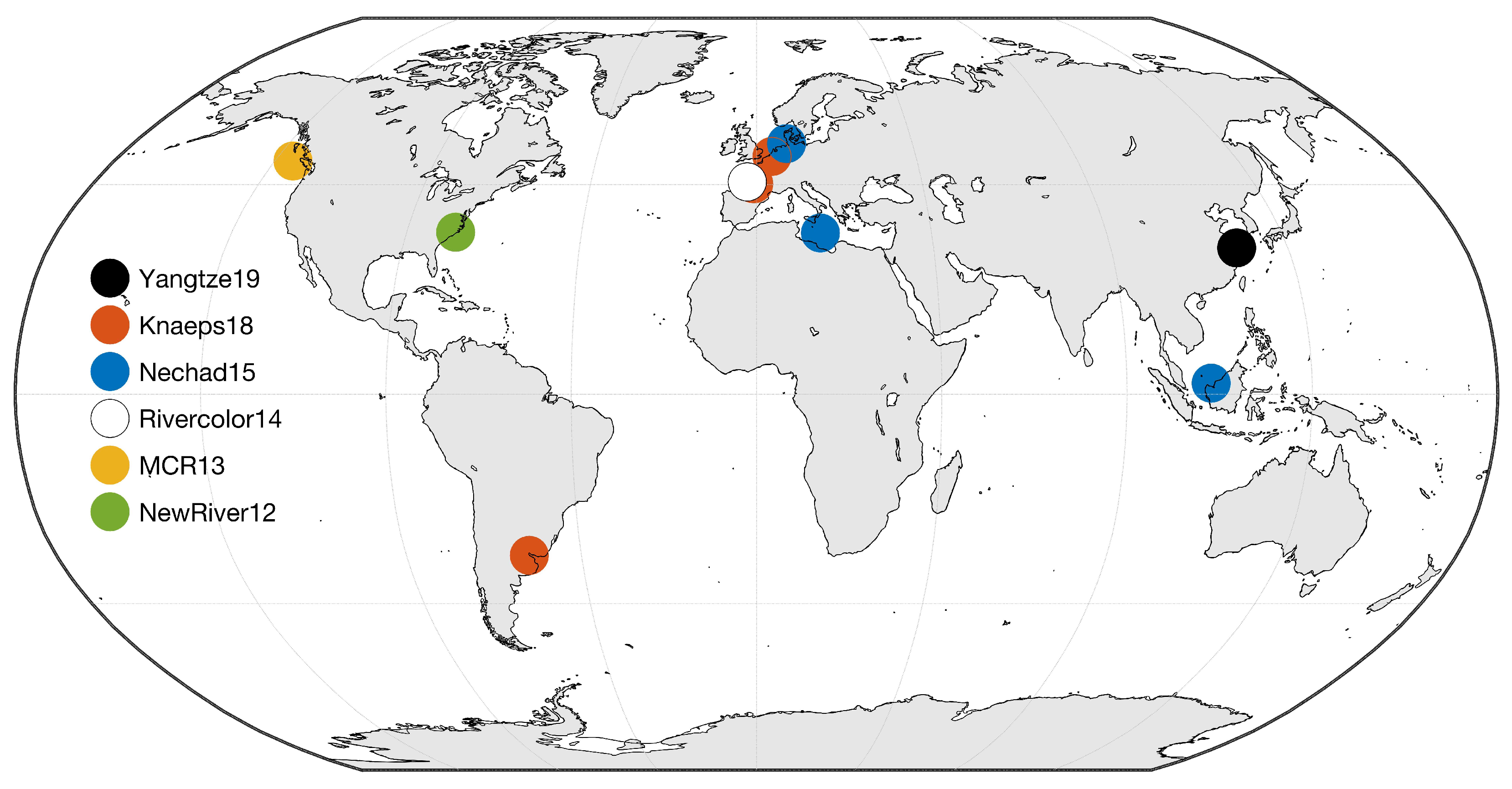
2.1. Data Sources
Field Data
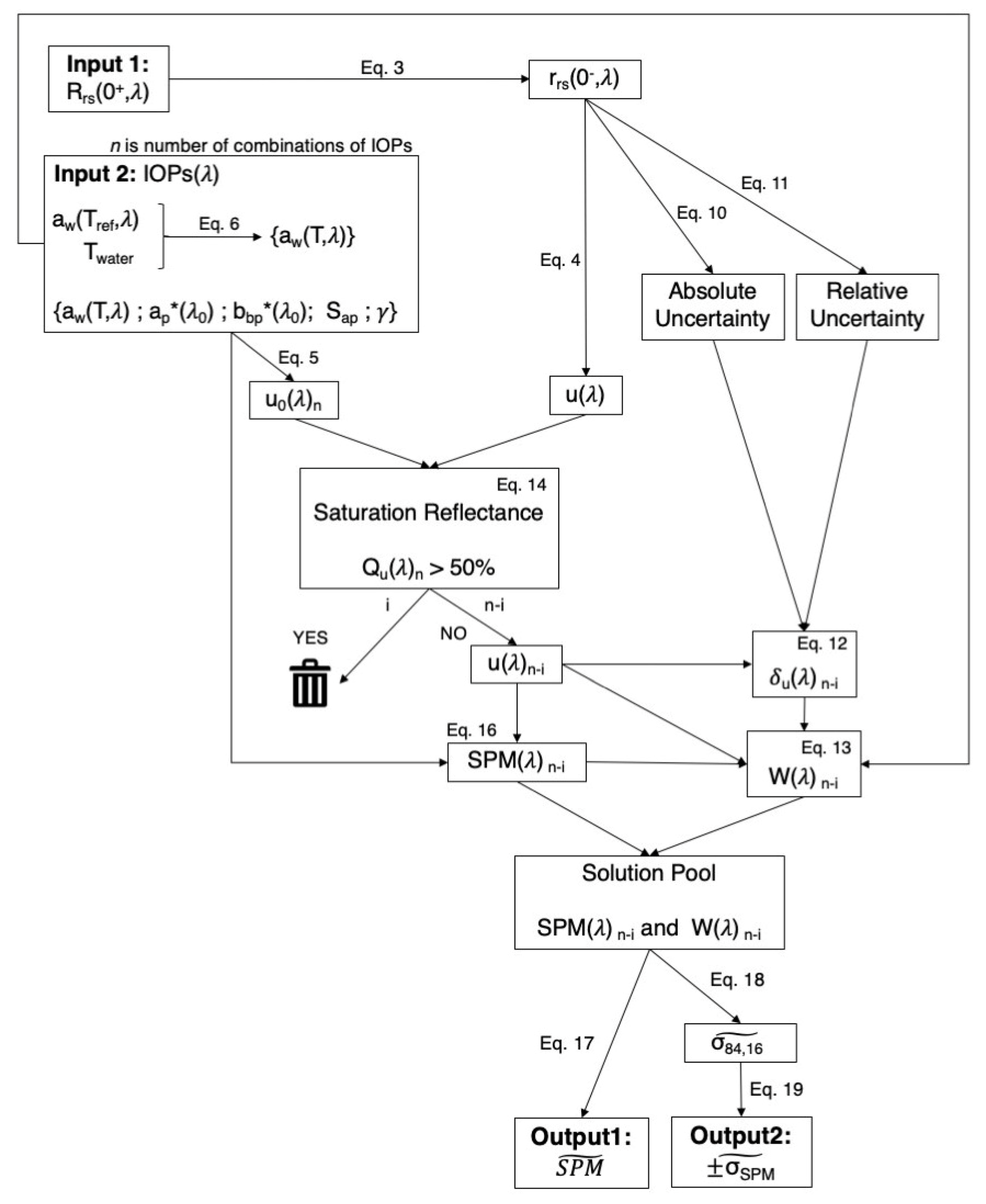
2.2. The MW algorithm
2.2.1. Approach
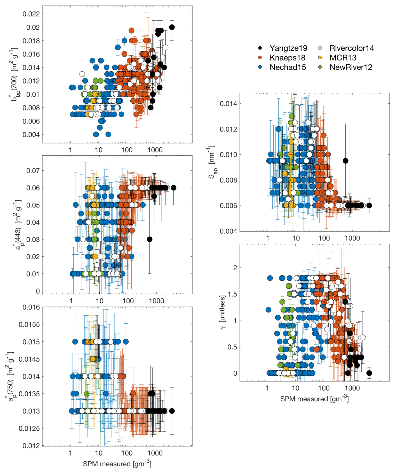
2.2.2. Parameterization of Inherent Optical Properties
2.2.3. Sensitivity of Solution to the Assumed Spectral Shape of Particulate IOPs
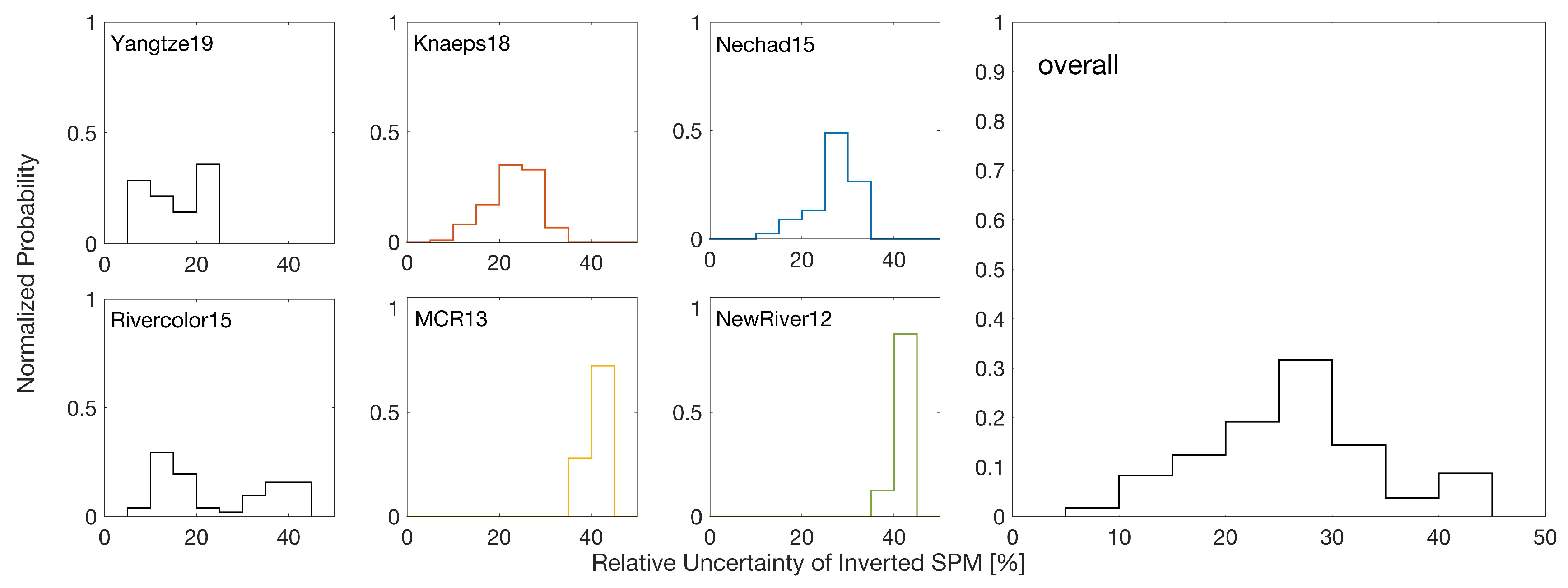
2.2.4. Uncertainties
2.2.5. The SPM Retrieval Approach
2.2.6. The IOP Retrieval Approach
2.3. Comparison to State-of-the-Art Algorithms
2.3.1. Nechad et al., 2010 Algorithm
2.3.2. Novoa et al., 2017 Algorithm
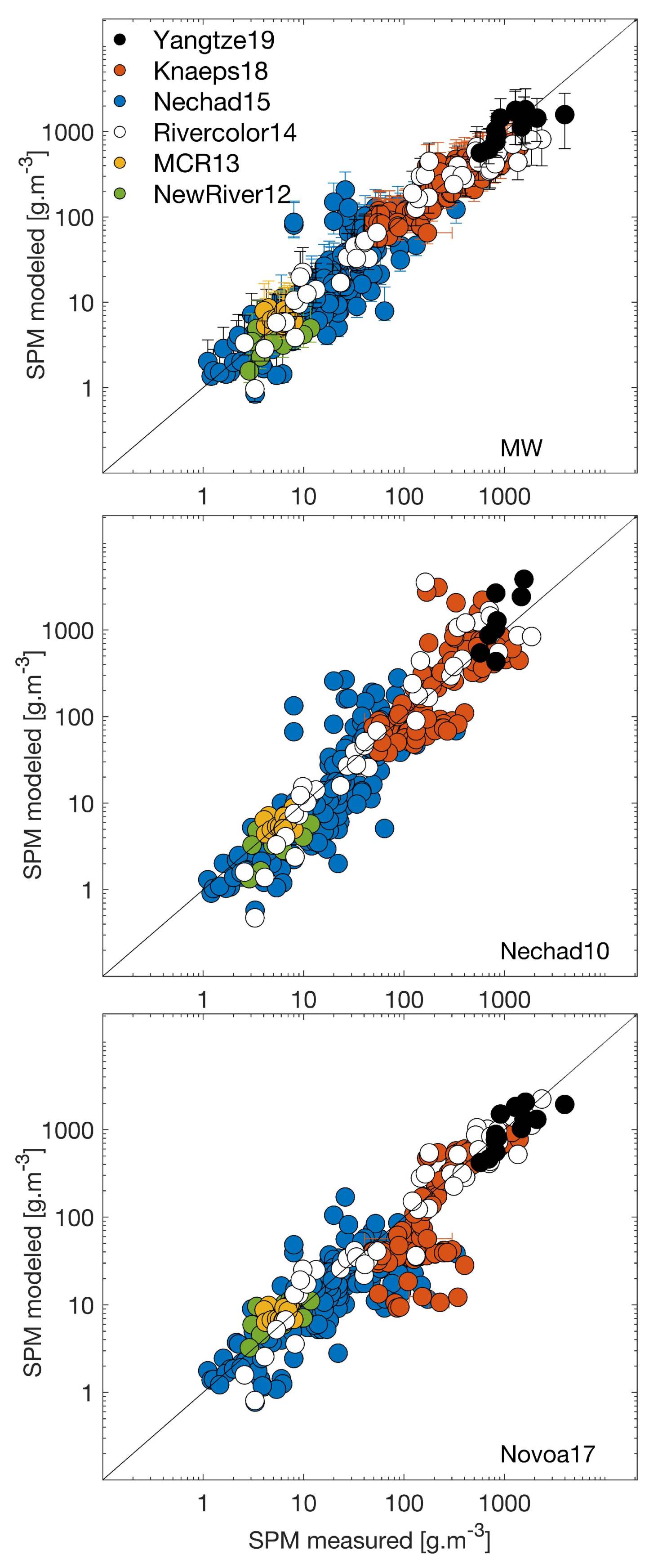
3. Results
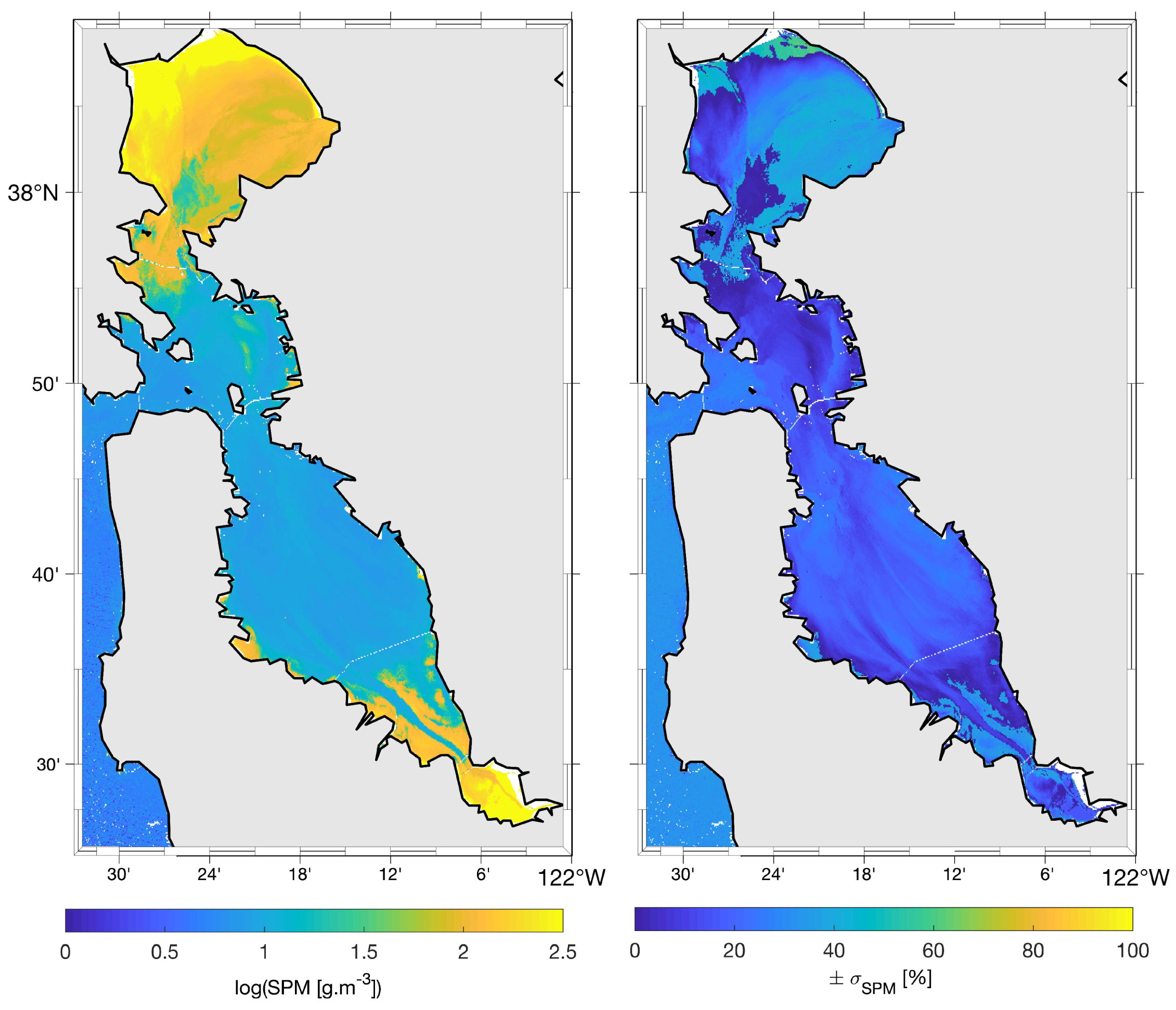
3.1. SPM Estimates
3.2. Estimates of IOP Parameters
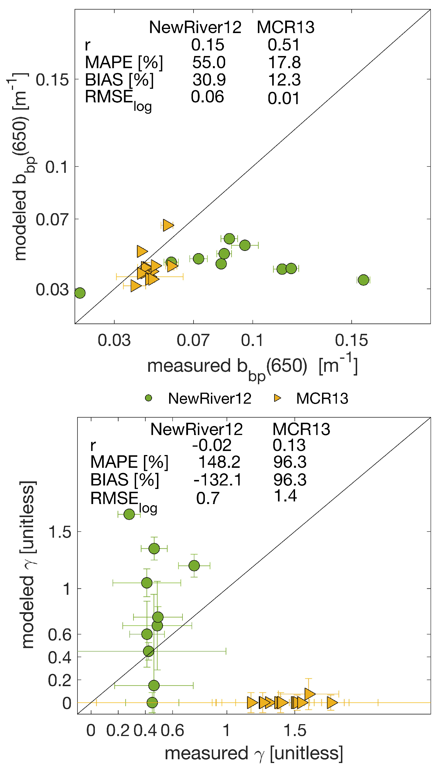
Validation of IOP Estimates
4. Discussion
4.1. Implications and Limitations of the MW Algorithm
4.2. Performance of the SPM Algorithms
5. Conclusions
Supplementary Materials
Author Contributions
Funding
Acknowledgments
Conflicts of Interest
References
- Tao, J.; Hill, P.S. Correlation of Remotely Sensed Surface Reflectance With Forcing Variables in Six Different Estuaries. JGR Ocean. 2019, 123, 9439–9461. [Google Scholar] [CrossRef]
- Stumpf, R.P. Sediment Transport in Chesapeake Bay During Floods: Analysis Using Satellite and Surface Observations. J. Coast. Res. 1988, 4, 1–15. [Google Scholar]
- Doxaran, D.; Froidefond, J.M.; Lavender, S.; Castaing, P. Spectral signature of highly turbid waters Application with SPOT data to quantify suspended particulate matter concentrations. Remote Sens. Environ. 2002, 81, 149–161. [Google Scholar] [CrossRef]
- Yu, X.; Lee, Z.; Shen, F.; Wang, M.; Wei, J.; Jiang, L.; Shang, Z. An empirical algorithm to seamlessly retrieve the concentration of suspended particulate matter from water color across ocean to turbid river mouths. Remote Sens. Environ. 2019, 235, 111491. [Google Scholar] [CrossRef]
- Tanaka, A.; Kishino, M.; Doerffer, R.; Schiller, H.; Oishi, T.; Kubota, T. Development of a Neural Network Algorithm for Retrieving Concentrations of Chlorophyll, Suspended Matter and Yellow Substance from Radiance Data of the Ocean Color and Temperature Scanner. Remote Sens. Environ. 2004, 60, 519–530. [Google Scholar] [CrossRef]
- Balasubramaniana, S.V.; Pahlevana, N.; Smitha, B.; Bindinge, C.; Schallesf, J.; Loiselg, H.; Gurlinh, D.; Grebi, S.; Alikasj, K.; Randlaj, M.; et al. Robust Algorithm for Estimating Total Suspended Solids (TSS) in Inland and Nearshore Coastal Waters. J. Coast. Res. 2020, in press. [Google Scholar] [CrossRef]
- Nechad, B.; Ruddick, K.G.; Park, Y. Calibration and validation of a generic multisensor algorithm for mapping of total suspended matter in turbid waters. Remote Sens. Environ. 2010, 114, 854–866. [Google Scholar] [CrossRef]
- Dogliotti, A.I.; Ruddick, K.G.; Nechad, B.; Doxaran, D.; Knaeps, E. A single algorithm to retrieve turbidity from remotely-sensed data in all coastal and estuarine waters. Remote Sens. Environ. 2015, 156, 157–168. [Google Scholar] [CrossRef]
- Han, B.; Loisel, H.; Vantrepotte, V.; Meriaux, X.; Bryere, P.; Ouillon, S.; Dessailly, D.; Xing, Q.; Zhu, J. Development of a semi-analytical algorithm for the retrieval of suspended particulate matter from remote sensing over clear to very turbid waters. Remote Sens. 2016, 8, 211. [Google Scholar] [CrossRef]
- Novoa, S.; Doxaran, D.; Ody, A.; Vanhellemont, Q.; Lafon, V.; Lubac, B.; Gernez, P. Atmospheric corrections and multi-conditional algorithm for multi-sensor remote sensing of suspended particulate matter in low-to-high turbidity levels coastal waters. Remote Sens. 2017, 9, 61. [Google Scholar] [CrossRef]
- Stumpf, R.P.; Pennock, J.R. Calibration of a General Optical Equation for Remote Sensing of Suspended Sedimentis in a Moderately Turbid Estuary. J. Geophys. Res. 1989, 94, 363–371. [Google Scholar] [CrossRef]
- Brando, V.E.; Dekker, A.G. Satellite Hyperspectral Remote Sensing for Estimating Estuarine and Coastal Water Quality. IEEE Trans. Geosci. Remote Sens. 2003, 41, 1378–1388. [Google Scholar] [CrossRef]
- Luo, Y.; Doxaran, D.; Ruddick, K.; Shen, F.; Gentili, B.; Yan, L.; Huang, H. Saturation of water reflectance in extremely turbid media based on field measurements, satellite data and bio-optical modelling. Opt. Express 2018, 26, 10435. [Google Scholar] [CrossRef] [PubMed]
- Knaeps, E.; Ruddick, K.G.; Doxaran, D.; Dogliotti, A.I.; Nechad, B.; Raymaekers, D.; Sterckx, S. A SWIR based algorithm to retrieve total suspended matter in extremely turbid waters. Remote Sens. Environ. 2015, 168, 66–79. [Google Scholar] [CrossRef]
- Babin, M.; Stramski, D.; Ferrari, G.M.; Claustre, H.; Bricaud, A.; Obolensky, G.; Hoepffner, N. Variations in the light absorption coefficients of phytoplankton, nonalgal particles, and dissolved organic matter in coastal waters around Europe. J. Geophys. Res. 2003, 108, 3211. [Google Scholar] [CrossRef]
- Zheng, G.; DiGiacomo, P. Uncertainties and applications of satellite-derived coastal water quality products. Prog. Oceanogr. 2017, 159, 45–72. [Google Scholar] [CrossRef]
- Shi, W.; Wang, M. Characterization of Suspended Particle Size Distribution in Global Highly Turbid Waters From VIIRS Measurements. J. Geophys. Res. Ocean. 2019, 124, 3796–3817. [Google Scholar] [CrossRef]
- Volpe, V.; Silvestri, S.; Marani, M. Remote sensing retrieval of suspended sediment concentration in shallow waters. Int. J. Remote Sens. 2011, 115, 44–54. [Google Scholar] [CrossRef]
- Melin, F.; Sclep, G.; Jackson, T.; Sathyendranath, S. Uncertainty estimates of remote sensing reflectance derived from comparison of ocean color satellite data sets. Remote Sens. Environ. 2016, 177, 107–124. [Google Scholar] [CrossRef]
- Melin, F. Uncertainties in Ocean Colour Remote Sensing; IOCCG Report Series; International Ocean Colour Coordinating Group: Hanover, NH, Canada, 2019. [Google Scholar]
- Boss, E.; Maritorena, S. Uncertainties in the Products of Ocean-Colour Remote. In Remote Sensing of Inherent Optical Properties; Lee, Z.-P., Ed.; Reports of the International Ocean-Colour Coordinating Group (IOCCG): Dartmouth, NS, Canada, 2006; Volume 5, Chapter 3; pp. 19–25. [Google Scholar]
- Nechad, B.; Ruddick, K.; Schroeder, T.; Blondeau-Patissier, D.; Cherukuru, N.; Brando, V.E.; Dekker, A.G.; Clementson, L.; Banks, A.; Maritorena, S.; et al. The CoastColour Round Robin datasets: A database to evaluate the performance of algorithms for the retrieval of water quality parameters in coastal waters. PANGEA 2015. [Google Scholar] [CrossRef]
- Knaeps, E.; Doxaran, D.; Dogliotti, A.; Nechad, B.; Ruddick, K.; Raymaekers, D.; Sterckx, S. The SeaSWIR dataset. Earth Syst. Sci. Data Discuss. 2018, 10, 1–15. [Google Scholar] [CrossRef]
- Jiang, B.; Fan, D.; Nguyen, D.V.; Ji, Q.; Ren, F.; Sun, F.; Li, J.; Qi, Y. Periodically decreasing of total Suspended Matter using satellites 1984–2017 in Yangtze river Estuary. In prep.
- Ruddick, K.G.; Cauwer, V.D.; Park, Y.J. Seaborne measurements of near infrared water-leaving reflectance: The similarity spectrum for turbid waters. Limnol. Ocean. 2006, 51, 1167–1179. [Google Scholar] [CrossRef]
- Werdell, P.J.; McKinna, L.I.; Boss, E.; Ackleson, S.G.; Craig, S.E.; Gregg, W.W.; Lee, Z.; Maritorena, S.; Roesler, C.S.; Rousseaux, C.S.; et al. An overview of approaches and challenges for retrieving marine inherent optical properties from ocean color remote sensing. Prog. Oceanogr. 2018, 160, 186–212. [Google Scholar] [CrossRef] [PubMed]
- Lee, T.N.; Smith, N. Volume transport variability through the Florida Keys tidal channels. Cont. Shelf Res. 2002, 22, 1361–1377. [Google Scholar] [CrossRef]
- Gordon, H.; Brown, J.W.; Brown, O.; Evans, R.H.; Smith, C.R.; Baker, K.; Clark, D.K. A semi-analytic radiance model of ocean color. J. Geophys. Res. Atmos. 1988, 93, 10909–10924. [Google Scholar] [CrossRef]
- Babin, M.; Morel, A.; Fournier-Sicre, V.; Fell, F.; Stramski, D. Light scattering properties of marine particles in coastal and open ocean waters as related to the particle mass concentration. Limnol. Oceanogr. 2003, 48, 843–859. [Google Scholar] [CrossRef]
- Jerlov, N.G. Optical Oceanography; Elsevier Oceanography Series; Elsevier Science: Amsterdam, The Netherlands, 2014; p. 193. [Google Scholar]
- Sullivan, S.A. Experimental Study of the Absorption in Distilled Water, Artificial Sea Water, and Heavy Water in the Visible Region of the Spectrum. J. Opt. Soc. Am. 1963, 53, 962. [Google Scholar] [CrossRef]
- Hale, G.M.; Querry, M.R. Optical Constants of Water in the 200 nm to 200 μm Wavelength Region. Appl. Opt. 1973, 12, 555. [Google Scholar] [CrossRef]
- Querry, M.R.; Cary, P.G.; Waring, R.C. Split-pulse laser method for measuring attenuation coefficients of transparent liquids: Application to deionized filtered water in the visible region. Appl. Opt. 1978, 17, 3587–3592. [Google Scholar] [CrossRef]
- Kou, L.; Labrie, D.; Chylek, P. Refractive indices of water and ice in the 0.65–2.5m spectral range. Appl. Opt. 1993, 32, 3531–3540. [Google Scholar] [CrossRef] [PubMed]
- Buiteveld, H.; Hakvoort, J.M.H.; Donze, M. The optical properties of pure water. SPIE Proc. Ocean Optics XII 1994, 2258, 174–183. [Google Scholar]
- Pope, R.M.; Fry, E.S. Absorption spectrum (380–700 nm) of pure water. Integrating cavity measurements. Appl. Opt. 1997, 36, 8710–8723. [Google Scholar] [CrossRef]
- Sullivan, J.M.; Twardowski, M.S.; Zaneveld, J.R.V.; Moore, C.M.; Barnard, A.H.; Donaghay, P.L.; Rhoades, B. Hyperspectral temperature and salt dependencies of absorption by water and heavy water in the 400–750 nm spectral range. Appl. Opt. 2006, 45, 5294–5309. [Google Scholar] [CrossRef] [PubMed]
- Rottgers, R.; McKee, D.; Utschig, C. Temperature and salinity correction coefficients for light absorption by water in the visible to infrared spectral region. Opt. Express 2014, 22, 25093. [Google Scholar] [CrossRef] [PubMed]
- Wang, P.; Boss, E.; Roesler, C. Uncertainties of inherent optical properties obtained from semi-analytical inversions of ocean color. Appl. Opt. 2005, 44, 4074–4085. [Google Scholar] [CrossRef]
- Boss, E.; Roesler, C. Over Constrained Linear Matrix Inversion with Statistical Selection. In Remote Sensing of Inherent Optical Properties; Lee, Z.-P., Ed.; Reports of the International Ocean-Colour Coordinating Group (IOCCG): Dartmouth, NS, Canada, 2006; Volume 5, Chapter 8; pp. 57–62. [Google Scholar]
- Qin, Y.; Brando, V.E.; Dekker, A.G.; Blondeau-Patissier, D. Validity of SeaDAS water constituents retrieval algorithms in Australian tropical coastal waters. Geophys. Res. Lett. 2007, 34, 1–4. [Google Scholar] [CrossRef]
- Blondeau-Patissier, D.; Tilstone, G.H.; Martinez-Vicente, V.; Moore, G.F. Comparison of bio-physical marine products from SeaWiFS, MODIS and a bio-optical model with in situ measurements from Northern European waters. J. Opt. A Pure Appl. Opt. 2004, 6, 875–889. [Google Scholar] [CrossRef]
- Slade, W.H.; Boss, E. Spectral attenuation and backscattering as indicators of average particle size. Appl. Opt. 2015, 54, 7264–7277. [Google Scholar] [CrossRef]
- Blondeau-Patissier, D.; Brando, V.E.; Oubelkheir, K.; Dekker, A.G.; Clementson, L.A.; Daniel, P. Bio-optical variability of the absorption and scattering properties of the Queensland inshore and reef waters, Australia. J. Geophys. Res. Ocean. 2009, 114. [Google Scholar] [CrossRef]
- Estapa, M.L. Photochemical Reactions of Particulate Organic Matter. Ph.D. Thesis, University of Maine, Orono, ME, USA, 2011. [Google Scholar]
- Burggraaff, O. Biases from incorrect reflectance convolution. Opt. Express 2020, 28, 13801–13816. [Google Scholar] [CrossRef] [PubMed]
- Cael, B.B.; Chase, A.; Boss, E. Information content of absorption spectra and implications for ocean color inversion. Appl. Opt. 2020, 59, 3971–3984. [Google Scholar] [CrossRef]
- Jackson, D.A. Stopping rules in principal components analysis: A comparison of heuristical and statistical approaches. Ecology 1993, 74, 2204–2214. [Google Scholar] [CrossRef]
- Loisel, H.; Vantrepotte, V.; Jamet, C.; Dat, D.N. Challenges and New Advances in Ocean Color Remote Sensing of Coastal Waters. Oceanogr. Res. 2013, 1–38. [Google Scholar] [CrossRef]
- Freeman, L.A.; Ackleson, S.G.; Rhea, W.J. Comparison of remote sensing algorithms for retrieval of suspended particulate matter concentration from reflectance in coastal waters. J. Appl. Remote Sens. 2017, 2, 046028. [Google Scholar] [CrossRef]
- Mason, J.D.; Cone, M.T.; Fry, E.S. Ultraviolet (250–550 nm) absorption spectrum of pure water. Appl. Opt. 2016, 55, 7163–7172. [Google Scholar] [CrossRef]
- Aly, K.M.; Esmail, E. Refractive index of salt water: Effect of temperature. Opt. Mater. 1993, 2, 195–199. [Google Scholar] [CrossRef]
- Austin, R.; Halikas, G. The Index of Refraction of Seawater; Technical Report; University of California: Oakland, CA, USA, 1976. [Google Scholar]
- Baker, K.; Smith, R.C. Bio-optical classification and model of natural waters. Limnol. Oceanogr. 1982, 27, 500–509. [Google Scholar] [CrossRef]
- Becquerel, J.; Rossignol, J. Spectral Absorption of Light and Heat by Pure Inorganic Substance and Miscellaneous Materials (Nonmetals). Int. Crit. Tables 1929, 5, 268–271. [Google Scholar]
- Bricaud, A.; Babin, M.; Morel, A.; Claustre, H. Variability in the chlorophyll-specific absorption coefficients of natural phytoplankton: Analysis and parameterization. J. Geophys. Res. 1995, 100, 13321–13332. [Google Scholar] [CrossRef]
- Fry, E.S.; Kattawar, G.W.; Pope, R.M. Integrating cavity absorption meter. Appl. Opt. 1992, 31, 2055–2065. [Google Scholar] [CrossRef] [PubMed]
- Irvine, W.M.; Pollack, J.B. Infrared optical properties of water and ice spheres. Icarus 1968, 8, 324–360. [Google Scholar] [CrossRef]
- Kopelevich, O.V. Optical properties of pure water in the 250–600 nm range. Opt. Spectrosc. 1976, 41, 391–392. [Google Scholar]
- Palmer, K.F.; Williams, D. Optical properties of water in the near infrared. J. Opt. Soc. Am. 1974, 64, 1107–1110. [Google Scholar] [CrossRef]
- Pope, R.M. Optical Absorption of Pure Water and Sea Water Using the Integrating Cavity Absorption Meter. Ph.D. Thesis, Texas A & M University, College Station, TX, USA, 1993. [Google Scholar]
- Segelstein, D.J. The Complex Refractive Index of Water. Ph.D. Thesis, University of Missouri–Kansas City, Kansas City, MO, USA, 1981. [Google Scholar]
- Smith, R.C.; Baker, K.S. Optical properties of the clearest natural waters (200–800 nm). Appl. Opt. 1981, 20, 177–184. [Google Scholar] [CrossRef]
- Sogandares, F.M. The Spectral Absorption of Pure Water. Ph.D. Thesis, Texas A & M University, College Station, TX, USA, 1991. [Google Scholar]
- Sogandares, F.M.; Fry, E.S. Absorption spectrum (340–640 nm) of pure water. Photothermal Measurements. Appl. Opt. 1997, 36, 8699–8709. [Google Scholar] [CrossRef]
- Zolotarev, V.M.; Mikhilov, B.A.; Alperovich, L.L.; Popov, S.I. Dispersion and absorption of liquid water in the infrared and radio regions of the spectrum. Opt. Spectrosc. 1969, 27, 430–432. [Google Scholar]
- Neeley, A.R.; Mannino, A. Inherent Optical Property Measurements and Protocols: Absorption Coefficient; IOCCG Ocean Optics and Biogeochemistry Protocols for Satellite Ocean Colour Sensor Validation, International Ocean Colour Coordinating Group: Hanover, NH, Canada, 2018. [Google Scholar]
- Neukermans, G.; Ruddick, K.; Bernard, E.; Ramon, D.; Nechad, B.; Deschamps, P.Y. Mapping total suspended matter from geostationary satellites: A feasibility study with SEVIRI in the Southern North Sea. Opt. Express 2009, 17, 14029–14052. [Google Scholar] [CrossRef]
- Neukermans, G.; Ruddick, K.; Loisel, H.; Roose, P. Optimization and quality control of suspended particulate matter concentration measurement using turbidity measurements. Limnol. Ocean. Methods 2012, 10, 1011–1023. [Google Scholar] [CrossRef]


| Dataset | SPM [g.m] | Temperature [C] | N | Site Location |
|---|---|---|---|---|
| Yangtze19 | 574–3981 | 21.2–25.6 | 16 | Yangtze River, CHI |
| Knaeps18 | 86.3–1400.5 | 17.5–21.5 | 72 | Gironde Estuary, FRA |
| 49.6–402.0 | 20 | 32 | Scheldt Estuary, BEL | |
| 48.3–110.0 | 17.4 | 33 | Rio del Plata, URY | |
| Nechad15 | 6.0–330.0 | 29 | 119 | Indonesia, IDN |
| 0.4–31.2 | 14 | 48 | North Sea | |
| Rivercolor14 | 2.58–2355.4 | 20 | 51 | Gironde Estuary, FRA |
| MCR13 | 1.5–4.9 | 15 | 33 | Columbia River, OR, USA |
| NewRiver12 | 2.9–11.8 | 21 | 16 | New River, NC, USA |
| Dataset | Instrument | Spectral Range [nm] | Method |
|---|---|---|---|
| Yangtze19 | ASD spectrometer | 400–1075 | L, L, L, , |
| Knaeps18 | ASD spectrometer | 355–1300 | L, L, L, , |
| Nechad15 | Trios RAMSES | 318.2–950.9 | L, L, E, , |
| Trios RAMSES | 350–850 | L, L, E, , | |
| Rivercolor14 | Trios RAMSES | 350–950 | L, L, E, , |
| MCR13 | WISP 3 | 400–800 | L, L, E, , ; |
| HyperSAS based calibration | |||
| NewRiver12 | HyperPro in buoy mode | 349–801.4 | L, E |
| Symbol | Description | Unit |
|---|---|---|
| a | Total absorption coefficient | m |
| Absorption by dissolved substances | m | |
| Absorption by non-algal particles | m | |
| Mass-specific non-algal particulate absorption coefficient | m.g | |
| Absorption of phytoplankton | m | |
| Absorption by water molecules | m | |
| Total backscattering coefficient | m | |
| Particulate backscattering coefficient | m | |
| Mass-specific particulate backscattering coefficient | m.g | |
| Backscattering by water molecules | m | |
| Downwelling irradiance | W.m | |
| Downwelling radiance reflected by Spectralon plaque | W.m.sr | |
| Downwelling sky radiance | W.m.sr | |
| Upwelling radiance | W m sr | |
| Water-leaving radiance | W.m.sr | |
| Above, below water surface | − | |
| band, band width | nm | |
| Q | Estimated saturation reflectance | − |
| Estimated uncertainty | sr | |
| Estimated uncertainty | − | |
| uncertainty range | g.m | |
| Weighted uncertainty range | g.m | |
| Weighted uncertainty | g.m | |
| Spectral weights | m.g | |
| weighted-median | g.m | |
| Exponent of exponential spectral shapes | nm | |
| T, | Temperature, reference temperature | C |
| Exponent of power-law spectral shape | − | |
| Temperature correction coefficient for absorption of water | mK | |
| Wavelength, reference wavelength | nm | |
| Nadir viewing angle | rad | |
| Azimuth angle | rad | |
| water-leaving reflectance | − |
| Parameter | Range | Reference |
|---|---|---|
| 0.01–0.06 | [15,22,41] | |
| 0.013–0.015 | [38] | |
| 0.002–0.021 | [29]; NewRiver12; MCR13 | |
| 0.006–0.014 | [22,29] | |
| 0–1.8 | [22,41,42,43,44]; NewRiver12; MCR13 |
| Switching Criteria | SPM Algorithm | Weighting Equation |
|---|---|---|
| < 0.007 | 130.1 | − |
| 0.016 < < 0.007 | + | |
| 0.08 < < 0.016 | 531.5 | − |
| 0.12 < < 0.08 | + | |
| > 0.12 | 3750 + 1751 | − |
| Dataset | N | Algorithm | r | MAPE [%] | BIAS [%] | RMSE |
|---|---|---|---|---|---|---|
| Yangtze19 | 14 | MW | 0.56 | 22.63 | −2.51 | 0.14 |
| Nechad10 | 0.18 | 174.40 | −46.83 | 0.16 | ||
| Novoa17 | 0.63 | 29.94 | 3.68 | 0.16 | ||
| Knaeps18 | 137 | MW | 0.88 | 27.40 | −2.95 | 0.16 |
| Nechad10 | 0.38 | 85.05 | −24.56 | 0.32 | ||
| Novoa17 | 0.88 | 45.17 | 23.93 | 0.41 | ||
| Nechad15 | 166 | MW | 0.66 | 65.60 | −24.71 | 0.30 |
| Nechad10 | 0.41 | 83.39 | −21.27 | 0.39 | ||
| Novoa17 | 0.34 | 52.90 | 0.51 | 0.35 | ||
| Rivercolor14 | 51 | MW | 0.87 | 37.45 | −1.43 | 0.22 |
| Nechad10 | −0.20 | 163.71 | 27.73 | 0.16 | ||
| Novoa17 | 0.91 | 41.89 | −11.92 | 0.22 | ||
| MCR13 | 18 | MW | 0.16 | 23.42 | −16.46 | 0.12 |
| Nechad10 | 0.30 | 18.11 | 1.31 | 0.10 | ||
| Novoa17 | 0.32 | 36.66 | −34.97 | 0.16 | ||
| NewRiver12 | 16 | MW | 0.46 | 34.96 | 26.39 | 0.22 |
| Nechad10 | 0.55 | 35.15 | 27.40 | 0.23 | ||
| Novoa17 | 0.61 | 41.57 | −36.64 | 0.17 |
| SPM Range [g.m] | N | Algorithm | r | MAPE [%] | BIAS [%] | RMSE |
|---|---|---|---|---|---|---|
| Overall | 402 | MW | 0.88 | 44.41 | −11.16 | 0.24 |
| Nechad10 | 0.23 | 92.47 | −14.12 | 0.23 | ||
| Novoa17 | 0.90 | 46.89 | 3.96 | 0.34 | ||
| SPM < 50 | 193 | MW | 0.60 | 59.47 | −22.54 | 0.28 |
| Nechad10 | 0.49 | 70.62 | −14.38 | 0.35 | ||
| Novoa17 | 0.60 | 48.00 | −15.96 | 0.26 | ||
| SPM > 50 | 209 | MW | 0.84 | 30.49 | −0.65 | 0.20 |
| Nechad10 | 0.20 | 112.65 | −13.87 | 0.11 | ||
| Novoa17 | 0.88 | 45.87 | 22.35 | 0.40 |
| Dataset | S | (443) | (750) | (700) | Site Location | |
|---|---|---|---|---|---|---|
| Yangtze19 | 0.006 [0.006–0.010] | 0.3 [0–1.8] | 0.06 [0.02–0.06] | 0.013 [0.013–0.015] | 0.014 [0.008–0.021] | Yangtze River, CHI |
| Knaeps18 | 0.006 [0.006–0.014] | 0.78 [0–1.8] | 0.060 [0.01–0.06] | 0.013 [0.013–0.015] | 0.012 [0.006–0.021] | Gironde Estuary, FRA (2012) |
| 0.006 [0.006–0.014] | 1.35 [0–1.8] | 0.060 [0.01–0.06] | 0.013 [0.013–0.015] | 0.014 [0.007–0.021] | Gironde Estuary, FRA (2013) | |
| 0.007 [0.006–0.014] | 1.61 [0.45–1.8] | 0.055 [0.01–0.06] | 0.013 [0.013–0.015] | 0.012 [0.009–0.017] | Scheldt Estuary, BEL | |
| 0.008 [0.006–0.014] | 1.8 [0–1.8] | 0.050 [0.01–0.06] | 0.013 [0.013–0.015] | 0.013 [0.009–0.017] | Rio del Plata, URY | |
| Nechad15 | 0.009 [0.006–0.014] | 1.3 [0–1.8] | 0.03 [0.01–0.06] | 0.013 [0.013–0.015] | 0.009 [0.004–0.020] | Indonesia, IDN |
| 0.009 [0.006–0.014] | 0.6 [0–1.8] | 0.028 [0.01–0.06] | 0.014 [0.013–0.015] | 0.008 [0.007-0.012] | North Sea | |
| Rivercolor14 | 0.006 [0.006–0.014] | 1.1 [0–1.8] | 0.06 [0.01–0.06] | 0.013 [0.013–0.015] | 0.012 [0.006–0.021] | Gironde Estuary, FRA |
| MCR13 | 0.007 [0.006–0.014] | 0 [0–0.5] | 0.058 [0.01–0.06] | 0.0145 [0.013–0.015] | 0.008 [0.007–0.010] | Columbia River, OR, USA |
| NewRiver12 | 0.009 [0.006–0.014] | 0.9 [0–1.8] | 0.01 [0.01–0.06] | 0.0132 [0.013–0.015] | 0.010 [0.008–0.012] | New River, NC, USA |
© 2020 by the authors. Licensee MDPI, Basel, Switzerland. This article is an open access article distributed under the terms and conditions of the Creative Commons Attribution (CC BY) license (http://creativecommons.org/licenses/by/4.0/).
Share and Cite
Tavora, J.; Boss, E.; Doxaran, D.; Hill, P. An Algorithm to Estimate Suspended Particulate Matter Concentrations and Associated Uncertainties from Remote Sensing Reflectance in Coastal Environments. Remote Sens. 2020, 12, 2172. https://doi.org/10.3390/rs12132172
Tavora J, Boss E, Doxaran D, Hill P. An Algorithm to Estimate Suspended Particulate Matter Concentrations and Associated Uncertainties from Remote Sensing Reflectance in Coastal Environments. Remote Sensing. 2020; 12(13):2172. https://doi.org/10.3390/rs12132172
Chicago/Turabian StyleTavora, Juliana, Emmanuel Boss, David Doxaran, and Paul Hill. 2020. "An Algorithm to Estimate Suspended Particulate Matter Concentrations and Associated Uncertainties from Remote Sensing Reflectance in Coastal Environments" Remote Sensing 12, no. 13: 2172. https://doi.org/10.3390/rs12132172
APA StyleTavora, J., Boss, E., Doxaran, D., & Hill, P. (2020). An Algorithm to Estimate Suspended Particulate Matter Concentrations and Associated Uncertainties from Remote Sensing Reflectance in Coastal Environments. Remote Sensing, 12(13), 2172. https://doi.org/10.3390/rs12132172