Abstract
In high-precision GPS precise point positioning (PPP) time transfer, errors caused by the effect of ionosphere delay have to be corrected. Usually the ionosphere-free combinations of the pseudo code and the carrier phase is used in GPS PPP data processing, and it effectively eliminates the effect of the first-order ionospheric delay. This study quantitatively analyzes the errors caused by higher-order ionospheric (Ion2+) delays in precise PPP time transfer. Data of two 7-day test periods, including low and moderate ionospheric conditions, from 20 stations located in middle- and low-latitude, were analyzed. The difference in clock solution with and without the Ion2+ correction, including the receiver clock solution and time-link clock solution, was deeply analyzed and discussed. The difference sequence shows a constant bias plus some variations with a diurnal variation. For the difference of the receiver clock solutions, the mean standard deviation of the variations is 3.92 ps in low-latitude, which is much larger than that of 2.59 ps in mid-latitude due to the influence of the larger ionospheric electron density on the low-latitude. The maximum constant bias reached more than 15 ps and was negative at most stations in the northern hemisphere, while it was positive at most stations located in the southern hemisphere. The difference in the time-link solutions correlates not only with time and region, but also with the length of the time-links. The largest difference in the long time-link SYDN-PTBB, BJNM-SYDN, AMC2-SYDN, etc., reaches more than 25 ps, while that of the short time-link IENG-PTBB, BRUX-PTBB, etc., is less than 3.5 ps. Therefore, the Ion2+ correction is necessary for high-precision PPP time transfer over long time-links, especially time-links made by one station located in the northern hemisphere and another located in the south hemisphere; however, it could be ignored for short time-links.
1. Introduction
Time transfer is based on the processing of transmitted time signals from one station to another. Dual-frequency Global Positioning System (GPS) signals have been successfully used for precise positioning and timing. The main methods of precise time transfer using GPS are common view (CV), all-in-view (AV), and precise point positioning (PPP). Compared to CV and AV, a 2–3 orders higher frequency stability can be obtained by the PPP, and it has a better reach than E-15–E-16 [1,2,3,4,5,6]. The current GPS PPP is used as a routine method for precise time and frequency transfer in many time laboratories around the world [1,2].
GPS PPP is a joint analysis of dual-frequency pseudo code and carrier phase observation from a single GPS station. It calculates a high-precision receiver coordinate and clock and tropospheric delay, among others. Ionospheric delay is an important error in GPS PPP positioning and timing application [7,8,9]. The first order ionospheric delay is usually removed almost completely (99%) by forming an dual-frequency ionosphere-free (IF) combination in PPP processing. However, the remaining ionospheric errors, that is the 2nd-order (Ion2) and 3rd-order (Ion3) delay terms, may cause centimeter-level errors in GPS measurements [9,10,11,12,13,14,15]. The goal of this paper is to evaluate the effect of the Ion2 and Ion3 (Ion2+) delay terms on GPS PPP time transfer.
In recent years, a large number of research results have focused on Ion2+ modeling and its impact on GPS global network processing. Hernandez-Pajares et al. (2007, 2014) and Hadas et al. (2017) conducted a systematic study of the Ion2 effect on the precise GPS satellite orbit and clock, receiver position and clock, tropospheric delay, etc. They concluded that the error caused by Ion2+ terms is under 5 mm for the orbit radial components, with a reach of about 2 cm for satellite clocks [12,15,16]. In other studies, Ion2+ terms were seen to cause a latitudinal shift of about 1 ~ 5 mm in static PPP coordinates under normal ionosphere conditions, and reaching up to −11 mm during high ionosphere conditions in low-latitude regions (<30°) [12,13,14,15,16,17,18,19,20,21]. For the kinematic PPP coordinates, the maximum effect is 0.8 cm for horizontal and more than 2.4 cm for vertical [22]. Meanwhile, Hernandez-Pajares et al. (2007, 2014) reported that the effect of Ion2+ on the receiver clock was at the level of 10 ps, and the effect of Ion2+ perturbations was significant [12,16]. Hoque et al. (2017) investigated the effect of overall Ion2+ terms on trans-ionospheric microwave propagation up to 100 GHz, which shows that the time delay due to the Ion2+ term is in the range of 1 × 10⁻¹³ s ~ 2 × 10⁻¹⁶ s at frequency 30 ~ 60 GHz.
In particular, the IERS Conventions 2010 recommends that the influence of Ion2+ terms should be taken into account for sub-centimeter (about 30 ps) level positioning; in addition, Section 9.4 describes the mathematical expression of the Ion2+ delay in GNSS [23]. In the second full reanalysis of all International GNSS Service (IGS) GPS observations collected since 1994, the calculation and application of Ion2 terms has been identified as one an important issue to be resolved [24].
Typically, Pireaux et al. (2009, 2010) reported that the effect of Ion2+ terms on the clock solution in CV time transfer reaches 10 ps under high ionospheric activity condition and around 15 ps under ionospheric stormy condition [25,26]. However, there is no set of coherent precise satellite orbits and clocks with Ion2+ correction to study the focus of the PPP time transfer at that specific time. On the basis of the above research results, higher-order ionospheric error must be corrected for the subnanosecond time and frequency transfer using microwave links [27].
The second full reanalysis of IGS (in 2017) provided precise satellite orbit and clocks with Ion2 correction by February 2015, which allowed us to implement a study on the error caused by Ion2+ in precise PPP time transfer. In view of this, the effect of the Ion2+ delay terms on PPP time transfer globally is investigated by comparing the clock solutions with and without Ion2+ terms correction. The methodology of PPP time transfer containing the Ion2+ terms is presented in Section 2. Section 3 describes the used data and the detailed processing strategy. Section 4 briefly analyzes the effect of Ion2+ on the global ionospheric map. Following that, a detailed analysis of the solutions with and without the Ion2+ terms corrections are made in Section 5. Finally, the conclusions are presented in Section 6.
2. Methodology
Starting from the basic observation equations of the pseudo code and carrier phase, this section presents the PPP model containing the Ion2 and Ion3 delay terms. The calculation method of the Ion2 and Ion3 delay terms is given as well.
Considering the ionospheric effect of the Ion2 and Ion3 delay terms, the observation equation of the pseudo code () and the carrier phase () can be expressed as [23]:
where is the geometrical distance of the receiver-satellite, is the speed of light, is the receiver clock offset, is the satellite clock offset, is the tropospheric delay, and is the wavelength and integer ambiguity of the carrier phase observation. is the frequency of the GPS signal in Hz, Hz, Hz. and is the combination of the multipath effect and measurement noise of the pseudo code and carrier phase observations, respectively. , , and identify the first-, second-, and third-order ionospheric delay, respectively, which can be written as [23]:
where is the number density of free electrons. is the total electron content (TEC) along the slant path from the satellite to station (expressed in TECU, 1 TECU = electrons/m2). B is a vector of the geomagnetic field at the ionospheric pierce point (IPP), which can be calculated using the International Geomagnetic Reference Field (IGRF) model [28]. is the angle between the satellite signal propagation direction and the vector B at IPP. is the maximum electron density at the altitude of the ionospheric.
In the actual processing, the second integral in formula (5) is neglected because it is usually two orders of magnitude smaller than the first integral for the GPS carrier frequency [23].
The STEC (slant TEC) can be generated by interpolation from the global ionosphere map of TEC (GIM-TEC). It may also be calculated by the smoothed dual-frequency code observations:
where and is the smoothed code observations of the GPS frequency L1 and L2, respectively. and is the DCB of the receiver and the satellite, respectively, which is the code bias caused by the hardware delay difference of different signals in satellite and receiver.
The can be expressed as a function of and the altitude of the ionospheric [23]:
where VTEC is the short for vertical TEC, is the mean radius of the Earth (6371 km), is correction factor, and is the zenith distance at the station [29]. Note that some empirical parameters are introduced in the numerical calculation, but the resulting errors are almost negligible.
Considering the Ion2 and Ion3 delay terms, IF combination of the pseudo code and carrier phase can be written as:
It can be seen that only the first-order ionospheric delay is removed, and the IF function still contains the Ion2 and Ion3 delay terms. Formulae (1), (2), (9), and (10) show that the Ion2 and Ion3 delay term of the pseudo code is two and three times that on the carrier phase, respectively.
According to the principle of classical least square method, the unknown vector to be estimated can be written as:
where is the vector of the estimated parameters, including receiver three-dimensional coordinate and clock, and tropospheric delay. is the coefficient matrix of the linear equation, is the weight matrix, and is the residual vectors. is the Ion2+ delay terms of the IF combination. is the effect of the Ion2+ delay terms on the receiver coordinate and clock, and the tropospheric delay, which can be considered as the effect transmitted by the error of the observation caused by the Ion2+ delay terms.
3. Data and Processing Strategy
3.1. Data
In order to show the response of the receiver clock to ionospheric spatial and temporal variations, it is necessary to select a number of GPS stations distributed reasonably. We selected 20 stations from the IGS tracking network (http://www.igs.org/network) according to the following criteria: (a) equipped with high-performance receivers and choke-ring antennas; (b) high-performance atomic clocks as frequency reference; and (c) distributed in middle- and low-latitude. This information is queried from the log files of each of the stations [24]. Figure 1 presents the detailed distribution of the 20 selected stations.
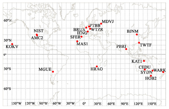
Figure 1.
Distribution of the 20 selected stations.
Regarding temporal variations, two 7-day test periods with different ionosphere activity characteristics were selected. The detailed information is as follows:
- ⚬
- The first test period: July 20–26, Day-of-year (Doy) 201–207, 2014, low ionospheric condition.
- ⚬
- The second test period: December 9–15, Doy 343–349, 2014, moderate ionospheric condition.
Figure 2 shows ionospheric conditions during the two test periods. The VTEC at the IPP (11.64°N, 92.71°E) above the PBRI station is extracted from the calculated GIM. The GIM processing strategy and results will be given in the next section. The cubic spline interpolation function is used to advance the sampling rate of 2 h to 15 min. Data on the disturbance storm time (DST) index and the solar radio flux at 10.7 cm (F10.7 index) were downloaded from the European Space Agency (ESA) website (http://space-env.esa.int/index.php), and the sampling rate is 1 h and 1 day, respectively. The F10.7 index represents a major parameter to describe the solar radiation intensity, which reflects the solar activity, expressed in solar flux units (sfu, 1 sfu =10−22 W·m−2·Hz−1). The DST index is used to assess the intensity of magnetic storm in middle- and low-latitude, expressed in nanoteslas (nT). We can see that the DST index in the first test period is the same with some small variation, but there is a weak geomagnetic disturbance event on Doy 346–347 in the second test period. The test periods cover low and moderate ionospheric conditions. The maximum VTEC of the second test period is almost two times larger than that of the first test period, which is the result of the stronger solar flux and geomagnetic activities in the second test period.
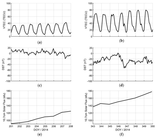
Figure 2.
Ionospheric conditions during the first test period (a), (c), (e) and the second test period (b), (d), (f). Vertical total electron content (VTEC) extracted from the final IGS global ionosphere map (IGS-GIM) at the ionospheric pierce point (IPP) above the station PBRI (11.64°N, 92.71°E) (a) and (b); the disturbance storm time index (c) and (d); the solar radio flux at 10.7 cm (e) and (f).
3.2. Processing Strategy
The raw data in Rinex-format (receiver independent exchange format) [30] preprocessing is the first step in our data processing, including gross error detection, cycle slip detection, and smoothing pseudo code with carrier phase observation. In the second step, the magnitudes of the Ion2+ delay terms effects on the range measurements is computed using the open program RINEX_HO, and generate the new Rinex files with the Ion2+ correction [10]. In order to be compatible with the updated data format, the IGRF model in the program has been upgraded from version 11 to version 12. The IGRF12 contains the post-process IGRF coefficients for 2014, not the predicted values in IGRF11 [28]. The precise STEC is extracted from the computed GIM in the next section. In the third step, RINEX files with and without the Ion2+ correction is processed in the daily static PPP mode, respectively, with the improved Bernese GNSS software Version 5.2 by National Time Service Center, Chinese Academy of Sciences (NTSC, CAS) for the international GNSS Monitoring and Assessment System (iGMAS) analysis center [31]. The detailed summary of the PPP processing strategy is given in Table 1.

Table 1.
Detailed summary of the PPP processing strategy.
The satellite clocks provided by IGS are referenced to an internal time scale, IGS Time scale (IGST), generated using a weighted algorithm based on the performance of the clock frequency in the GPS satellites and IGS stations [32]. As a matter of course, the PPP receiver clock solutions calculated using the IGS satellite clocks is also referenced to IGST. After getting all receiver clock solutions referenced to IGST, time transfer between receiver A and receiver B can be computed using the following equation:
where and is the clock solution of receiver A and receiver B, respectively.
Finally, on comparison, the difference sequence of the clock solution with and without Ion2+ delay terms, including receiver clock solution and time-link clock solution, is analyzed.
The most important thing to notice here is that we processed the observations with and without Ion2+ delay terms corrections using a consistent set of precise satellite orbits and clocks with the Ion2 delay terms correction provided by the second full reanalysis of IGS. It can avoid the effect caused by different orbit and clock of satellites.
4. GIM Determination
When calculating the Ion2+ delay terms in Section 3.2, the GIM-TEC at the IPP was used. In this section, we calculate and analyze the GIM using GPS dual-frequency observations from 220 IGS stations distributed globally. Figure 3 presents the distribution of all stations used to calculate GIM. We can see that there are fewer stations in the southern hemisphere and marine areas due to fewer selectable stations. The ionospheric model data processing is carried out by the Bernese GNSS software version 5.2 [29]; a detailed processing strategy is shown in Table 2. In addition, three days of data are processed as a combination period, and the solution of the middle day as the final GIM results. To separate the satellite DCB and receiver DCB, zero mean conditions for all satellite were introduced as a constraint [29,33]. Here, the cut-off elevation angle is set to 10°, which is different from that set to 7.5° in the PPP processing strategy. This is done to mitigate the influence of low-elevation ionospheric spatial anomalies. The calculated results include the GIM in IONEX (IONosphere map EXchange) format [34] with a spatial resolution of 2.5° × 5° (latitude × longitude) and a temporal resolution of 2 h, and the satellite DCB and receiver DCB.
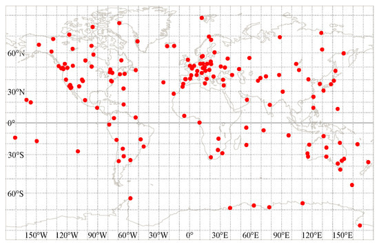
Figure 3.
Distribution of the stations for global ionospheric modeling.
Table 2.
Detailed summary of global ionospheric modeling.
The comparison with the IGS-GIM final products verifies the computed GIM using the raw observations, and the average difference in the second test period is shown in Figure 4. To save space, the difference plot for each day is not shown here. Table 3 gives the standard deviation (STD) of the difference between the computed GIM and the IGS GIM. It can be clearly seen that the difference in low latitude is much larger than that in middle and high latitudes. According to the statistical values, the global average difference is 2.78 TECU, and the STD of all satellites DCB is less than 0.05 ns. Through the above analysis, the results indicated that the precision of the computed GIM is close to that of the final IGS GIM.
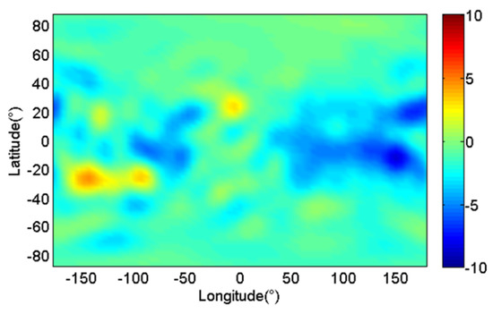
Figure 4.
Average difference between the IGS-GIM and the computed global ionosphere map (GIM) during doy 344–349 in 2014.
Table 3.
Standard deviation (STD) between IGS-GIM and the computed GIM during the doy 344–349 in 2014.
Furthermore, we evaluate the effect of the Ion2+ delay terms on the precision of the GIM. A specific approach is to first use the above-mentioned method to generate the Rinex files with the Ion2+ correction of all stations, then calculate the GIM with the raw Rinex files and the Ion2+ correction Rinex files, respectively, and finally the solutions of two experiments are compared. In this calculation, the same stations and processing strategy are used to exclude the influence of other factors.
Figure 5 shows the average difference between the GIM with and without Ion2+ correction in the second test period. The latitude range in the figure is set to 60° S ~ 60° N, which is consistent with the distribution of the stations (Figure 1) applied to time transfer research. We can observe that the difference is below 0.4 TECU in most regions. From each set of solution in the second test period, the average difference is about 0.4 TECU–0.7 TECU, and the maximum difference is less than 1.4 TECU. IGS official data show that the precision of IGS GIM is 2 ~ 8 TECU [33]. Therefore, the effect of the Ion2+ terms on the current GIM precision is limited. It is feasible to use the GIM calculated by the raw observations to calculate Ion2+ terms.
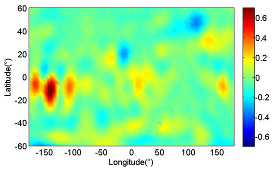
Figure 5.
Average difference between the GIM with and without Ion2+ correction during doy 344–349 in 2014.
5. Results Comparison and Analysis
A comparative analysis was performed for the computed results of the observations with and without Ion2+ correction, first, in terms of the effects of Ion2+ on the L1 and L2 observations, then in terms of their impact on receiver clocks solution and time transfer.
5.1. Effect on Observations
The computed Ion2 and Ion3 correction on carrier phase observations for the L1 and L2 frequency at station PBRI (11.64°N, 92.71°E) in the two test periods are shown in Figure 6. The Ion2_L1 and Ion3_L1 represents the Ion2 and Ion3 correction for the carrier phase on L1 signal, respectively, and the Ion2_L2 and Ion3_L3 are also similar. The sequence on doy 201 is interrupted due to missing data. The diurnal variation of the Ion2 and Ion3 terms with time appear clearly, which are similar to that of VTEC shown in Figure 2. The daily peak value of Ion2 and Ion3 delay terms appeared in the late afternoon (local time) and the minimum appeared before sunrise.
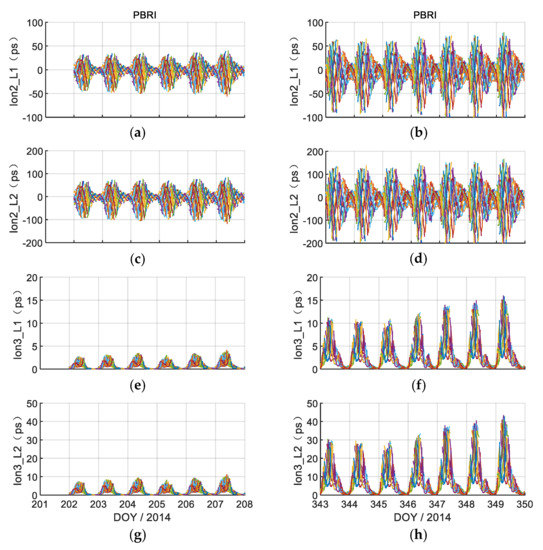
Figure 6.
Correction of the Ion2 and Ion3 terms on L1 and L2 carrier phase observations at PBRI station (11.64°N, 92.71°E) in two test periods. The first test period: (a), (c), (e), and (g); the second test period: (b), (d), (f), and (h). The Ion2 correction: (a)–(d), and the Ion3 correction: (e)–(h).
According to Equation (2), the effect of the Ion2 terms on L2 observation is 2.11 times that on L1, and that of the Ion3 terms on L2 observation is 2.71 times that on L1. The results of the station PBRI shown in Figure 6 coincides well with the above theoretical calculation values. The effect of Ion2 term on observation is almost 10 times higher than that of Ion3 term. In the second test period, for the PBRI station, the variation range of Ion2 terms effect reaches about −100 ps ~ 70 ps and −200 ps ~150 ps for L1 and L2 observations, while those of Ion3 are about 0 ps ~ 15 ps and 0 ps ~ 40 ps, respectively. There is a slight fluctuation in the Ion2 and Ion3 delay terms’ sequence during the magnetic storm on Doy 346–347, 2014.
From the comparison of the first and second test periods, the effect of Ion2+ on observations under moderate ionospheric condition is much larger than that under low ionosphere condition. Specifically, the correction of the Ion2 terms in the second test period is about three times larger than that in the first test period. With Figure 2 analysis, it was mainly due to the larger TEC and the stronger geomagnetic activity in the second test period than that in the first test period.
A comprehensive analysis of all stations shows that the effect of the Ion2+ terms on the observation is time- and latitude-dependent. The Ion2+ effects on the observation from the station KAT1 and PBRI located in low latitude is more serious than that from other stations located in the middle latitude. Affected by the magnetic induction intensity, the Ion2 terms sequences of the stations near the equator are basically symmetrical, but it becomes positive or negative in the middle latitude. The sign in the Ion2 delay terms depends crucially on the geometry between the satellite and receiver, more specifically, it depends on the in Formula (4). The Ion3 terms sequence of all stations is always positive. As the I3 term is very small and the magnitude is basically equivalent to the I2 term noise, the follow-up analysis will not be separated.
5.2. Effects on Receiver Clock Solutions
The receiver clocks were estimated in daily batches using PPP processing strategy introduced in Section 3.2, for all test stations and all test periods, with and without corrections of the Ion2+ terms. As the receiver clock with and without Ion2+ correction refer to the IGST, the effect of the Ion2+ terms on the receiver clocks can be evaluated by comparing the solutions with and without the Ion2+ terms correction.
Figure 7 shows the difference between receiver clock solutions with and without Ion2+ terms correction for the PTBB, IENG, AMC2, and PBRI stations on the doy 345 in 2014. As you can see by the curves of each station, there is significant variation trend in one day, but these are not entirely consistent. This is largely because the horizontal in each subplot is GPS Time (GPST), not Local Time (LT). For example, the longitude difference of PTBB and IENG station is less than 3°, their LT is close, and the variation trend of their curves looks pretty much the same. The peak value of the difference curves of all stations appear in late afternoon LT, which is the response of ionospheric VTEC.
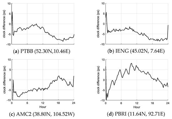
Figure 7.
Difference between the receiver clock with and without Ion2+ terms correction for the PTBB (a), IENG (b), AMC2 (c), and PBRI (d) stations on the doy 345 in 2014.
Figure 8 shows the difference between the receiver clock solutions with and without the Ion2+ terms correction over the two test periods at seven stations located at different latitudes. In the figure, the left column (subplot (a)~(g)) and the right column (subplot (h)~(n)) represent the first test period and the second test period, respectively. We can see that there are some discontinuities in the difference series due to the missed data in the Rinex files. Two obvious phenomena of a long convergence process in the daily PPP clocks and discontinuities at the day boundaries were observed. These phenomena remain difficult, which affects the application of PPP in time transfer [2,4].
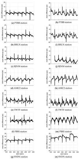
Figure 8.
Difference between receiver clock solutions with and without Ion2+ terms correction at the station PTBB (a) and (h), BRUX PTBB (b) and (i), BJNM PTBB (c) and (j), AMC2 PTBB (d) and (k), TWTF PTBB (e) and (l), PBRI PTBB (f) and (m), and SYDN PTBB (g) and (k) over the first test period (left column, (a)–(g)) and the second test period (right column, (h)–(n)).
For each station, the daily variation showed very good repeatability, which is very similar to the diurnal variation of the Ion2+ terms described in Figure 6. In the first test period with low ionosphere conditions, the difference series and its variation range of all stations are far smaller than that in the second test period with moderate ionospheric condition. Here, taking station TWTF (24.95 N, 121.16 E)) as an example (subplot (e) and (l) in Figure 8), the difference range is from about 0 ps to less than 10 ps in the first test period, but its reach is from about 0 ps to greater than 15 ps in the second test period. It is worth noting that the effect of the Ion2+ disturbances on the Doy 346–347 on the PPP clock is not significant.
The difference series for all stations show a constant bias plus some variations. Figure 9 presents the STD and biases of the difference series between the receiver clock solutions with and without Ion2+ terms correction in the second test period. In the subplot (a), the red bar represents the STD of the difference, and the black dot represents the latitude of the stations. The black bar in the subplot (b) represents the magnitude of difference bias. As a convergence exists when calculating the receiver clocks, the first 30 min of each day are not used in the STD and bias calculation.
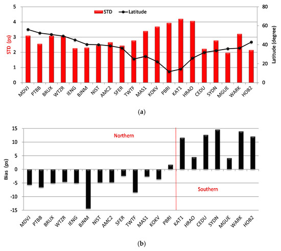
Figure 9.
STD (a) and bias (b) of differences series between the receiver clock solutions with and without Ion2+ terms correction for all stations during the second test period. The red line in the subplot (b) is the dividing line between the northern and southern hemisphere.
The STD of the difference series based on all stations is found to be closely related to the latitude of the station, and increases with decrease in latitude. The mean STD of six stations located in the low latitudes (<30°) is about 3.92 ps and that of 14 stations located in the mid-latitudes (30°–60°) is about 2.59 ps.
The constant biases of most stations located in the northern hemisphere are negative (clock increase), and those of most stations located in the southern hemisphere are positive (clock decrease). This is consistent with the obvious positive or negative of the Ion2 terms correction at each station, but its magnitude has no obvious change rules.
In Figure 8 and Figure 9, the peak of the difference reaches more than 15 ps for the BJNM, KAT1, and SYDN stations, and the statistical value is −14.40 ± 2.31 ps, −11.63 ± 4.21 ps, and 14.61 ± 2.78 ps (bias ± STD), respectively. However, the statistical value of the three stations in the first test period is −8.10 ± 1.65 ps, 2.46 ± 2.24 ps, and 6.36 ± 2.06 ps, respectively, which is much smaller than that in the second test period. This corresponds to the moderate and low ionospheric condition given in Figure 2.
5.3. Effects on Time Transfer
Choose the PTBB station as a central node to form 19 time-links with other stations. Figure 10 shows the difference between clock solutions with and without Ion2+ terms correction for the time-links IENG-PTBB, AMC2-PTBB, PBRI-PTBB, and SYDN-PTBB on doy 345 in 2014. Figure 11 presents a comparison of the clock solution of the six time-links with and without Ion2+ terms correction over the two test periods. The difference curve is a combination of the clock difference curve of two receivers, which shows more complex change trend in one day, but the diurnal variation is obvious in the whole test process. It can be seen that the effect of the Ion2+ terms on the solution of time-links IENG-PTBB and BRUX-PTBB is the least and less than 2 ps, while that of time-link SYDN-PTBB is the largest and up to more than 26 ps. The reasonable explanation of this phenomenon will be given in the follow-up analysis.
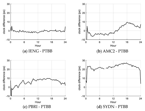
Figure 10.
Differences between clock solutions for time-link IENG-PTBB (a), AMC2-PTBB (b), PBRI-PTBB (c), and SYDN-PTBB (d) with and without Ion2+ corrections on doy 345 in 2014.
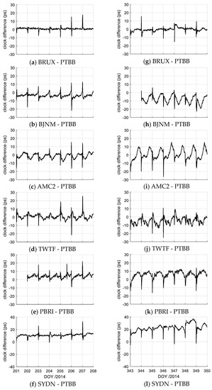
Figure 11.
Differences between clock solutions for time-link BRUX-PTBB (a) and (g), BJNM-PTBB (b) and (h), AMC2-PTBB (c) and (i), TWTF-PTBB (d) and (j), PBRI-PTBB (e) and (k), SYDN-PTBB (f) and (l) with and without Ion2+ terms correction during the first test period (left column, (a)–(f)) and the second test period (right column, (g)–(l)).
The difference in the time-links clock solution with and without Ion2+ terms correction also shows a constant bias plus some variations. Figure 12 presents the difference STD (a) and bias (b) of 19 time-links station (k)—PTBB in the second test period, where k represents one of the other 19 stations. In subplot (a), the red bar represents the STD of the difference, the blue bar represents the length of the time-links, and the black dot represents the latitude of the stations. The black bar in the subplot(b) represents the bias of the difference. We can see that the effect of the Ion2+ on the time-links solution correlates not only temporally and spatially, but also with the length of the time-links.
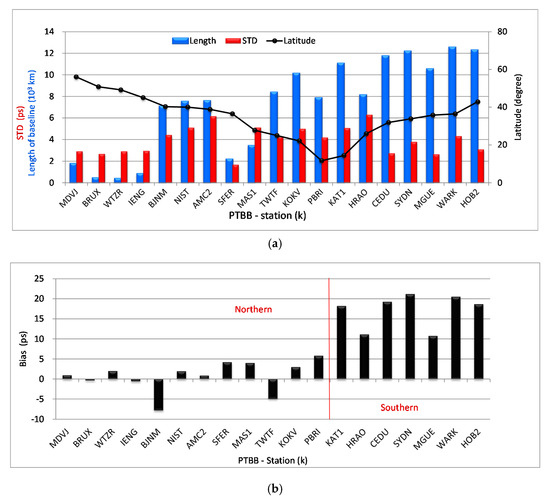
Figure 12.
STD (a) and bias (b) of the differences between the clock solutions of the time-link station (k)-PTBB with and without the Ion2+ corrections during the second test period. k refers to 19 selected stations. The red line in the subplot (b) is the dividing line between the northern and southern hemisphere.
The mean STD of 6 time-links of PTBB—another station located in the low latitudes (<30°)—is about 4.98 ps and that of 13 time-links of PTBB—another station located in the mid-latitudes (30°–60°)—is about 3.48 ps.
The STD of the short time-links IENG-PTBB, BRUX-PTBB, WTZR-PTBB, SFER-PTBB, and MDVJ-PTBB is less than 2.95 ps, which is much smaller than that of the long time-links BJNM-PTBB (4.71 ps), AMC2-PTBB (6.33 ps), and NIST-PTBB (6.34ps). However, in Figure 9a, the STD of PPP clocks’ difference for stations BJNM, AMC2, and NIST were similar to those of stations IENG, BRUX, WTZR, SFER, and MDVJ. This is mainly because these stations are located in middle latitudes, but the length of the time-link IENG-PTBB, BRUX-PTBB, WTZR-PTBB, SFER-PTBB, and MDVJ-PTBB is less than 2180 km, which is much shorter than that of BJNM-PTBB (7089km), AMC2-PTBB (7589km), and NIST-PTBB (7532km). The shorter the time-links, the stronger the spatial and temporal correlation of the Ion2+ delay terms at two stations, and the smaller the effect of the Ion2+ terms on time transfer.
Figure 12b shows that the constant bias of the time link made by PTBB and another station located in the northern hemisphere is relatively small, while that of PTBB and another station located in the southern hemisphere is relatively large. This resulted from the opposite sign of the receiver clock solutions in the southern and northern hemisphere shown in Figure 9b. Here, taking the SYDN and BJNM stations with the largest difference in the receiver clock as an example, the constant bias of the time-link SYDN-PTBB reached 21.21 ps, while that of the time-link BJNM-PTBB is only −7.79 ps.
To clarify this further, we added the analysis of the time-links BJNM-SYDN (8224.9 km) and AMC2-SYDN (11059.6 km); the difference of the two time-links clock solution with and without the Ion2+ correction is shown in Figure 13. Table 4 gives the average and STD of the time-links clock solution difference with and without Ion2+ correction. We can see that the peak of the difference is over 35 ps for the link BJNM-SYDN and over 25 ps for the link AMC2-SYDN in the second test period, which is much more than that of the links BJNM-PTBB, AMC2-PTBB, and so on. Compared with the results in Figure 12, the average value and STD of the time-link BJNM-SYDN and AMC2-SYDN are also larger.
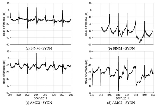
Figure 13.
Differences between clock solutions for time-link BJNM–SYDN (a) and (b), AMC2-SYDN (c) and (d) with and without Ion2+ corrections in the first (left column, (a) and (c)) and second test periods (right column, (b) and (d)).
Table 4.
Statistics of the difference between the time-links clock solution with and without the Ion2+ correction.
According to the comprehensive analysis of the two test period, the difference variation rule of the difference between the time-links clock solution with and without the Ion2+ correction in the first test period is consistent with that in the second test period. From Table 4, we can also see that the constant bias and STD of the time-links in the first test period is much smaller than that in the second test period.
Based on the above analysis, the Ion2+ terms’ correction was necessary for high-precision PPP time transfer over a long time-link, especially as the time-link is made by one station located in the northern hemisphere and another in the southern hemisphere, and it could be ignored for short time-links. The spatial and temporal variation (diurnal, seasonal, sunspot activity, etc.) of the ionosphere is quite complicated, requiring meticulous follow-up research.
6. Conclusions
In this study, the errors caused by Ion2+ delay terms in PPP time transfer was investigated. We selected 20 IGS stations equipped with high performance receivers, antennas, and H-maser atomic clocks. In addition, two 7-day test periods with different ionosphere conditions was considered. The clock solutions with and without the Ion2+ corrections were compared and thoroughly analyzed.
Overall, the effects of the Ion2+ terms on the receiver clocks and time-links clock solutions are time- and region-dependent. The difference in clock solutions, including receiver clock and time-links clock solution, with and without the Ion2+ terms correction show a constant bias plus some variations with a diurnal variation. The effect of the Ion2+ terms on the current GIM-TEC precision is limited and can be ignored.
For the difference of the receiver clocks in the moderate ionospheric condition, the STD of the variations is 3.92 ps and 2.59 ps in the low-latitudes and mid-latitudes, respectively. The constant bias of most stations in the northern hemisphere was negative, while that of most stations in the southern hemisphere was positive. The largest effect of Ion2+ on the receiver clocks reached more than 15 ps at the BJNM, SYDN, and KAT1 station.
The difference in the time-links clock solution correlates not only with time and region but also with the length of the time-links. In moderate ionospheric condition, the largest difference in the long time-link SYDN-PTBB, BJNM-SYDN, AMC2-SYDN, etc., reaches more than 25 ps, while that of the short time-link IENG-PTBB, BRUX-PTBB, etc., is less than 3.5 ps.
Therefore, the Ion2+ correction is necessary for subnanosecond PPP time transfer over long links, especially those made by one station located in the northern hemisphere and another in the south hemisphere, but it could be ignored for short links.
Author Contributions
H.Y. put forward the research ideas, conducted the experiments, and wrote the manuscript. Z.Z. conducted some data collection and analysis. X.Y., B.S., and W.Q. contributed to the discussions and revised the manuscript. All authors have read and agreed to the published version of the manuscript.
Funding
This research was funded by the CAS “Light of West China” Program (XAB2017B11, Y915YR1801) and the National Natural Science Foundation of China (No.11703033).
Acknowledgments
The authors sincerely thank IGS, CODE, ESA and National Space Science Data Center, National Science & Technology Infrastructure of China for providing the available data and precise products, as well as the Astronomical Institute of the University of Bern (AIUB) and NTSC iGMAS Analysis Center for making the processing software available.
Conflicts of Interest
The authors declare no conflict of interest.
References
- Petit, G.; Harmegnies, A.; Mercier, F.; Perosanz, F.; Loyer, S. The time stability of PPP links for TAI. In Proceedings of the Joint Meeting European Frequency and Time Forum and IEEE International Frequency Control Symposium, San Francisco, CA, USA, 2–5 May 2011; pp. 1041–1045. [Google Scholar]
- Petit, G.; Kanj, A.; Loyer, S.; Delporte, J.; Mercier, F.; Perosanz, F. 1 × 10⁻¹⁶ frequency transfer by GPS PPP with integer ambiguity resolution. Metrologia 2015, 52, 301–309. [Google Scholar] [CrossRef]
- Defraigne, P.; Guyennon, N.; Bruyn, C. GPS time and frequency transfer: PPP and phase-only analysis. Int. J. Navig. Obs. 2008, 175468. [Google Scholar] [CrossRef]
- Defraigne, P.; Aerts, W.; Pottiaux, E. Monitoring of UTC(k)’s using PPP and IGS real-time products. GPS Solut. 2015, 19, 165–172. [Google Scholar] [CrossRef]
- Zhang, P.; Tu, R.; Zhang, R.; Gao, Y.; Cai, H. Combining GPS, BeiDou, and Galileo Satellite Systems for Time and Frequency Transfer Based on Carrier Phase Observations. Remote Sens. 2018, 10, 324. [Google Scholar] [CrossRef]
- Ge, Y.; Dai, P.; Qin, W.; Yang, X.; Zhou, F.; Wang, S.; Zhao, X. Performance of Multi-GNSS Precise Point Positioning Time and Frequency Transfer with Clock Modeling. Remote Sens. 2019, 11, 347. [Google Scholar] [CrossRef]
- Su, K.; Jin, S.; Hoque, M. Evaluation of Ionospheric Delay Effects on Multi-GNSS Positioning Performance. Remote Sens. 2019, 11, 171. [Google Scholar] [CrossRef]
- Rose, J.; Watson, R.; Allain, D.; Mitchell, C. Ionospheric corrections for GPS time transfer. Radio Sci. 2014, 49, 196–206. [Google Scholar] [CrossRef]
- Zhang, J.; Gao, J.; Yu, B.; Sheng, C.; Gan, X. Research on Remote GPS Common-View Precise Time Transfer Based on Different Ionosphere Disturbances. Sensors 2020, 20, 2290. [Google Scholar] [CrossRef]
- Marques, H.; Monico, J.; Aquino, M. RINEX_HO: Second-and third-order ionospheric corrections for RINEX observation files. GPS Solut. 2011, 15, 305–314. [Google Scholar] [CrossRef]
- Petrie, E.; Hernandez-Pajares, M.; Spalla, P.; Moore, P.; King, M. A review of higher order ionospheric refraction effects on dual frequency GPS. Surv. Geophys. 2011, 32, 197–253. [Google Scholar] [CrossRef]
- Hernandez-Pajares, M.; Aragon-Angel, A.; Defraigne, P.; Bergeot, N.; Prieto-Cerdeira, R.; Garcia-Rigo, A. Distribution and mitigation of higher-order ionospheric effects on precise GNSS processing. J. Geophys. Res. Solid Earth 2014, 119, 3823–3837. [Google Scholar] [CrossRef]
- Zhang, X.; Ren, X.; Guo, F. Influence of higher-order ionospheric delay correction on static precise point positioning. Inf. Sci. Wuhan Univ. 2013, 38, 883–887. [Google Scholar]
- Cai, C.; Liu, G.; Yi, Z.; Cui, X.; Kuang, C. Effect analysis of higher-order ionospheric corrections on quad-constellation GNSS PPP. Meas. Sci. Technol. 2019, 30, 2. [Google Scholar] [CrossRef]
- Hadas, T.; Krypiak-Gregorczyk, A.; Hernández-Pajares, M.; Kaplon, J.; Paziewski, J.; Wielgosz, P.; Garcia-Rigo, A.; Kazmierski, K.; Sosnica, K.; Kwasniak, D.; et al. Impact and implementation of higher-order ionospheric effects on precise GNSS applications. J. Geophys. Res. B Solid Earth 2017, 122, 9420–9436. [Google Scholar] [CrossRef]
- Hernandez-Pajares, M.; Juan, J.; Sanz, J.; Orus, R. Correction to “second-order ionospheric term in GPS: Implementation and impact on geodetic estimates”. J. Geophys. Res. Atmos. 2007, 112, B08417. [Google Scholar] [CrossRef]
- Liu, Z.; Li, Y.; Guo, J.; Li, F. Influence of higher-order ionospheric delay correction on GPS precise orbit determination and precise positioning. Geod. Geodyn. 2016, 7, 369–376. [Google Scholar] [CrossRef]
- Hoque, M.; Jakowski, N. Higher order ionospheric effects in precise GNSS positioning. J. Geod. 2007, 81, 259–268. [Google Scholar] [CrossRef]
- Elsobeiey, M.; El-Rabbany, A. On Modelling of Second-Order Ionospheric Delay for GPS Precise Point Positioning. J. Navig. 2012, 65, 59–72. [Google Scholar] [CrossRef]
- Jiang, W.; Deng, L.; Li, Z.; Zhou, X.; Liu, H. Effects on noise properties of GPS time series caused by higher-order ionospheric corrections. Adv. Space Res. 2014, 53, 1035–1046. [Google Scholar] [CrossRef]
- Banville, S.; Sieradzki, R.; Hoque, M.; Wezka, K.; Hadas, T. On the estimation of higher-order ionospheric effects in precise point positioning. GPS Solut. 2017, 21, 1817–1828. [Google Scholar] [CrossRef]
- Zhang, S.; Wang, X.; Huang, L.; Yin, F. Impact of Second Order Ionosphere Delays for GPS Kinematic Precise Point Positioning Applications. Acta Geodaetica et Cartographica Sinica. 2018, 47, 45–53. [Google Scholar]
- Boehm, J.; Hernandez-Pajares, M.; Hugentobler, U.; Hulley, G.; Mercier, F.; Niell, A.; Pavlis, E. Chapter 9: Models for Atmospheric Propagation Delays. In IERS Technical Note No. 36; IERS Conventions; IERS: Washington, DC, USA, 2010. [Google Scholar]
- Johnston, G.; Riddell, A.; Hausler, G. The international GNSS Service. In Springer Handbook of Global Navigation Satellite Systems; Teunissen, P.J., Montenbruck, O., Eds.; Springer International Publishing: Cham, Switzerland, 2017; pp. 967–982. [Google Scholar]
- Pireaux, S.; Defraigne, P.; Wauters, L.; Bergeot, N.; Baire, Q.; Bruyninx, C. Influence of ionospheric perturbations in GPS time and frequency transfer. Adv. Space Res. 2009, 45, 1101–1112. [Google Scholar] [CrossRef]
- Pireaux, S.; Defraigne, P.; Wauters, L.; Bergeot, N.; Baire, Q.; Bruyninx, C. Higher-order ionospheric effects in GPS time and frequency transfer. GPS Solut. 2010, 14, 267–277. [Google Scholar] [CrossRef]
- Hoque, M.; Jakowski, N.; Berdermann, J. Transionospheric Microwave Propagation: Higher-Order Effects up to 100 GHz; Intech Open Science Open Minds: London, UK, 2017; pp. 15–38. [Google Scholar]
- Thébault, E.; Finlay, C.C.; Beggan, C.D.; Alken, P.; Aubert, J.; Barrois, O.; Bertrand, F.; Bondar, T.; Boness, A.; Brocco, L.; et al. International Geomagnetic Reference Field: The 12th generation. Earth Planet Space 2015, 67, 79. [Google Scholar] [CrossRef]
- Dach, R.; Lutz, S.; Walser, P.; Fridez, P. Bernese GNSS Software Version 5.2; User Manual; Astronomical Institute, Universtiy of Bern: Bern, Switzerland, 2015. [Google Scholar]
- Gurtner, W.; Estey, L. RINEX: The Receiver Independent Exchange Format Version 2.11; Astronomical Institute, University of Bern: Bern, Switzerland, 2007. [Google Scholar]
- Yang, H.; Yang, X.; Zhang, Z.; Zhao, K. High-Precision Ionosphere Monitoring Using Continuous Measurements from BDS GEO Satellites. Sensors 2018, 18, 714. [Google Scholar] [CrossRef] [PubMed]
- Senior, K.; Koppang, P.; Ray, J. Developing an IGS time scale. IEEE Trans. Ultrason. Ferroelectr. Freq. Control 2003, 50, 585–593. [Google Scholar] [CrossRef] [PubMed]
- Zhang, Q.; Zhao, Q. Analysis of the data processing strategies of spherical harmonic expansion model on global ionosphere mapping for moderate solar activity. Adv. Space Res. 2019, 63, 1214–1226. [Google Scholar] [CrossRef]
- Schaer, S.; Gurtner, W.; Feltens, J. IONEX: The IONosphere Map EXchange format version 1. In Proceedings of the IGS Analysis Center Workshop, Darmstadt, Germany, 9–11 February 1998; pp. 233–247. [Google Scholar]


© 2020 by the authors. Licensee MDPI, Basel, Switzerland. This article is an open access article distributed under the terms and conditions of the Creative Commons Attribution (CC BY) license (http://creativecommons.org/licenses/by/4.0/).