Article

Rapid Flood Mapping and Evaluation with a Supervised Classifier and Change Detection in Shouguang Using Sentinel-1 SAR and Sentinel-2 Optical Data

1
School of Remote Sensing and Geomatics Engineering, Nanjing University of Information Science and Technology, Nanjing 210044, China
2
Jiangsu Engineering Center for Collaborative Navigation/Positioning and Smart Applications, Nanjing 210044, China
3
Shanghai Astronomical Observatory, Chinese Academy of Science, Shanghai 200030, China
*
Author to whom correspondence should be addressed.
Remote Sens. 2020, 12(13), 2073; https://doi.org/10.3390/rs12132073
Submission received: 15 May 2020 / Revised: 17 June 2020 / Accepted: 25 June 2020 / Published: 27 June 2020
(This article belongs to the Special Issue Land Use/Cover Change Detection with Geospatial Technologies)

Abstract

:
Rapid flood mapping is crucial in hazard evaluation and forecasting, especially in the early stage of hazards. Synthetic aperture radar (SAR) images are able to penetrate clouds and heavy rainfall, which is of special importance for flood mapping. However, change detection is a key part and the threshold selection is very complex in flood mapping with SAR. In this paper, a novel approach is proposed to rapidly map flood regions and estimate the flood degree, avoiding the critical step of thresholding. It converts the change detection of thresholds to land cover backscatter classifications. Sentinel-1 SAR images are used to get the land cover backscatter classifications with the help of Sentinel-2 optical images using a supervised classifier. A pixel-based change detection is used for change detection. Backscatter characteristics and variation rules of different ground objects are essential prior knowledge for flood analysis. SAR image classifications of pre-flood and flooding periods both take the same input to make sense of the change detection between them. This method avoids the inaccuracy caused by a single threshold. A case study in Shouguang is tested by this new method, which is compared with the flood map extracted by Otsu thresholding and normalized difference water index (NDWI) methods. The results show that our approach can identify the flood beneath vegetation well. Moreover, all required data and data processing are simple, so it can be popularized in rapid flooding mapping in early disaster relief.

Graphical Abstract

1. Introduction

Flooding is one of the most frequent and destructive natural hazards, which often causes property and life loss [1,2]. Satellite remote sensing plays an important role in all phases of hazard monitoring and management [3]. The traditional remote sensing of flood monitoring is still difficult due to the lack of data with sufficient acquisition frequency and timeliness [4], while synthetic aperture radar (SAR) systems offer the possibility to operate in day and night time [5]. Optical satellite images contain rich information in their bands [6], which have a preferable result in the classification of ground cover [7]. However, optical satellite images are vulnerable to weather conditions, and have poor quality during the period of disaster because it is always cloudy and rainy during that time. SAR images are independent of weather conditions, so they are the best choice under cloudy and rainy weather. The digital number (DN) values of SAR images show the backscatter characteristics of ground objects, but this has a bad result in the classification of ground cover due to its inadequacy of information [8]. However, the change in backscatter coefficients can sensitively reveal the change in backscatter properties and the state of ground objects. In particular, the backscatter coefficient increases due to flooding in all SAR bands over vegetated areas [9].
There were several studies on flood mapping using SAR images: (1) the threshold of SAR backscattering values; (2) RGB composition; and (3) classification techniques. The threshold selection of SAR backscattering values in flood mapping can be divided into two categories: (a) A single threshold value is used to separate flood and non-flood regions. The change detection of water bodies during pre-flood and flooding periods is normally used. Li et al. [7] proposed a two-step automatic change detection chain for rapid flood mapping based on Sentinel-1 SAR images, which only dealt with the negative change caused by open water in rural areas. This approach can only detect completely inundated areas, but cannot identify slightly inundated areas. A harmonic model-based approach and the alternative change detection were proposed to derive the flood extent and the Otsu thresholding method was applied in the change image to determine a threshold value [10]. However, a single threshold to distinguish flood and non-flood regions was not comprehensive enough to extract the changes caused by flooding because the backscatter values changed significantly; (b) Multiple threshold values are used to separate flood and non-flood regions with some proposed comprehensive models to select different thresholds for different land covers. Long et al. [11] proposed an approach for flood change detection and threshold selection to delineate the extent of flooding for the Chobe floodplain in the Caprivi region of Namibia, which can identify flooding in vegetation, but only two thresholds were used to extract inundated area and inundated vegetation. Pulvirenti et al. [12] used SAR data to map floods in agricultural and urban environments with interferometric coherence, a digital elevation model (DEM), and the land cover map as auxiliary data. A threshold selection is always complex and accompanied by algorithm innovation, which requires a good knowledge of mathematics.
A few researchers used classifiers with SAR images to extract inundated areas to avoid the critical step of thresholding. Amitrano et al. [8] exploited Sentinel-1 ground range detected (GRD) products with an unsupervised method for rapid flood mapping, and classic co-occurrence measurements combined with amplitude information were used for a fuzzy classification system without a threshold selection. Benoudjit et al. [13] proposed an approach to rapidly map the flood extent using a supervised classifier and both a pre-event SAR image and an optical Sentinel-2 image were used to train the supervised classifier to identify the inundation from the flooded SAR image. It can be processed in an automatic way, but only identified the completely inundated regions. Change detection using RGB composition is also a common approach. Dual polarized Sentinel-1 SAR images were used to map and monitor flooding in Kaziranga National Park [14]. Francisco et al. [15] used RGB composition and thresholding to monitor flooding with Sentinel-1 data in the Ebro River. The approach is based on the RGB color model, which processes the data to suit the model and get the best result, while this process is always subjective.
Although numerous efforts on flood mapping using SAR images were obtained, it was still challenging to use the Sentinel-1 SAR images as a powerful tool for flood mapping, especially for flood degree evaluation, which is an unsolved problem in current studies. SAR images show the backscatter characteristics of different ground objects. Each object has different backscatter characteristics in different inundated states, and the backscatter characteristics of one object in a certain flooding state is equal to another object’s backscatter characteristics in the normal state (not inundated). If the SAR images of pre-flood and flooding periods are both classified according to the same rule, the ground objects’ normal backscatter characteristics and the change of classes in the same position between two SAR images show the change in backscatter. Flood information can be extracted from the change with the variation rules of different ground objects, meaning that we can convert the change detection of ground objects’ backscatter to the change detection of land cover classification. In this paper, a novel approach is proposed to extract flooding regions and evaluate flooding extent from Sentinel-1 SAR images with the help of optical Sentinel-2 images, which converts the change detection of thresholding to backscatter classifications. The approach focuses on pixel-based change detection and a supervised classifier. A supervised classifier is used to ensure the SAR image classifications based on the same rule. Instead of other information, such as texture information, the optical Sentinel-2 images are used to improve the accuracy of land cover classification. In order to compare our approach with other traditional approaches, the Otsu thresholding method based on SAR images and the NDWI index method based on optical images are also applied in some cases. In Section 2, the study area and the data are described, the detailed methodology is described in Section 3, a case study and the results are presented in Section 4, and finally conclusions are given in Section 5.

2. Study Area and Data

2.1. Study Area

Shouguang City was selected as the study area (see Figure 1) because of its flooding history in summer over the past few years. It is famous and important as intensive vegetable cultivation areas located in Shandong Province, China. Its terrain is flat with many rivers, and Mihe River flows through the whole area. There are several reservoirs at its upstream. The average annual precipitation in Shouguang is about 593.8 mm, and the seasonal precipitation is highly concentrated in summer.
Shouguang suffered a severe rainstorm during Typhoon Rumbia in August 2018. The rainstorm started on 17 August 2018 and became heaviest on 20 August 2018 due to Typhoon Rumbia. The water discharge from upstream reservoirs made the flood heavier for a longer period. The water discharged along the Mihe River to the Bohai Sea, so riverbank villages were seriously damaged. The case study is tested in Kouzi Village in Shouguang City, which was one of the worst-hit areas. The village mainly consists of farmland and residential areas, and there is also a river and two intersecting major roads. The farmland can be broken down into farmland without plastic sheds and farmland with plastic sheds. There are mainly buildings and pathways in the residential areas. Therefore, there are five categories for classification: water bodies, roads, constructions, farmland without plastic sheds, and farmland with plastic sheds.

2.2. Data

Sentinel-1 data are free and have high resolution, which provide level 1 ground range detected (GRD) products. GRD products consist of focused SAR data that have been detected, multi-looked, and projected to ground range using an Earth ellipsoid model. GRD products are widely used in studying the backscattering of land cover and monitoring water bodies [16]. Different polarizations observed by Sentinel-1 show different detection sensitivities to the land surface [17,18]. Vertical-Horizontal polarization (VH) has a stronger return over areas with volume scattering and Vertical-Vertical polarization (VV) has stronger returns specular scattering. Therefore, both VV and VH are used to enrich the band information. A radar system with multiple polarizations provides more information on inundated vegetation areas than single-polarized SAR. Backscatter is generally lower for cross-polarization because the depolarization does not result from ideal corner reflectors.
The flood started on 17 August 2018 and became heaviest on 20 August 2018 and then receded gradually during the next week. The available GRD products on 20 August and 26 August 2018 were downloaded as the flooding period images. GRD products on 2 August 2018 were the nearest available images without rain during the 12 h before imaging. So the GRD products of Sentinel-1 on 2 August 2018 were downloaded as the pre-flood period images. To get the performances of rapid flooding mapping and evaluation during different rainfalls, the GRD products of Sentinel-1 on 21 July 2018 and 27 July 2018 were also downloaded for comparative tests. More detailed information about the images is shown in Table 1.
Sentinel-2 contributes to a variety of services that rely on multispectral high-spatial resolution optical observations over global terrestrial surfaces, which provides optical images with high resolution. Sentinel-2 provides 12 bands, including: coastal aerosol, blue, green, red, four vegetation red edge bands, near infrared (NIR), water vapor, and three short-wave infrared (SWIR) bands. Only blue, green, and red bands are used in this paper for land cover classification. Sentinel-2 images on 10 August 2018 are downloaded, which are of high quality in a non-flooding condition. Their full information is shown in Table 2.
Images from Planet are used here for comparison. Planet is also called Planet Labs, which is a satellite group consisting of many micro-satellites. Its products have high coverage rates, standard spectral resolution, high spatial resolution, and high time resolution. It provides four bands: red, green, blue, and NIR. The normalized difference water index (NDWI) is used here to extract the inundated area. Three Planet images were downloaded, which were the nearest to the SAR image date. Their full information is shown in Table 3.

3. Methodology

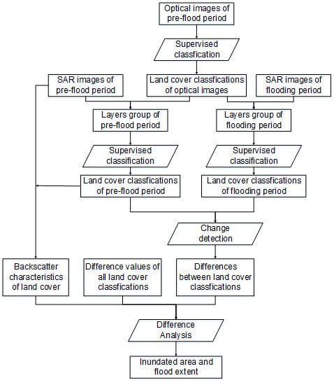
3.1. Method of Flood Mapping

The core idea of this methodology is the supervised classifier and change detection. The same supervised classifier and classification rules are applied in both SAR images of pre-flood and flooding periods, so the variations of backscatter can be extracted from the change detection results of the two SAR image classifications. Taking the variation rule of different objects as a criterion, the flood extent can be obtained from the change detection results. The detailed steps are shown below and the flowchart of the entire processing chain is presented in Figure 2.
(1)
Determine the land cover categories in the study area;
(2)
Download high-quality optical images and GRD images of the pre-flood and flooding period whose date is closest to the flood event. The dates of these two images may be different but must contain a flood;
(3)
Get the land cover classification based on the optical images with a supervised classification method, which is called normal optical classification;
(4)
Combine the GRD images of the pre-flood period with the normal optical classification into a layer group, and get the backscatter classification of the pre-flood period with a supervised method based on the layer group;
(5)
Combine the GRD images of the flooding period with the normal optical classification into a layer group, and get the backscatter classification of the flooding period with a supervised method based on the layer group;
(6)
Compute the average backscatter coefficient of each category based on the backscatter classification of the pre-flood period and arrange them in ascending order, which is one of the pieces of prior knowledge for flood mapping and evaluation;
(7)
The number of each category is the nth power of two and the two backscatter classification results are remarked in number according to the order of their average backscatter;
(8)
The other piece of prior knowledge is the backscatter variation rules of different classes;
(9)
Detect change information between the two backscatter classification results with the pixel-based method;
(10)
Determine the flood extent according to the prior knowledge in steps (6) and (8).

3.1.1. SAR Image Processing

GRD products provide amplitude and intensity bands with both VV and VH. The images are processed into sigma bands during radiometric, calibration, geometric, and speckle filtering. Because the change detection requires that all the layers are normalized, GRD products are finally processed into Gamma bands. Xin et al. [19] established several statistical models about the power transformation of SAR images to get some certain distributions, which was independent of image distribution. The Gamma index is processed in Equation (1) to show the backscatter better and avoid noise information caused by a negative number, and the processed Gamma index is named S_Gamma.
S _ Gamma = 100 × G a m m a ,
where Gamma refers to Gamma band.

3.1.2. Supervised Classification

There are three steps involving a classifier. The first is to get the land cover classification based on optical images, and the next two are SAR image classifications. The optical images are used to get the initial land cover classification, which is called normal optical image classification. Three bands (red, green and blue) of Sentinel-2 are three predictors for this classification. Sentinel-1 SAR images are used to get the backscatter classification of the pre-flood and flooding periods. The processed S_Gamma bands of both VV and VH and the normal optical classification are three predictors for classification. Samples of each category for the two classifications must be the pixels where each ground object is not in a flooding condition.
The random forest classifier is used here for classification, which is an ensemble learning method for classification, regression, and other tasks and operates by constructing a multitude of decision trees during the training time and outputting the class as the mode of the classes (classification) or mean prediction (regression) of the individual trees [20]. The random forest classification (RFC) has been applied successfully in ecological land cover studies [21]. The Random Forest Classification Toolbox in ENVI 5.3.1 is used in this study to train the model and get the classification results.

3.1.3. Backscatter Characteristics and Variation Rules of Ground Objects

The backscatter characteristics of each category are important prior knowledge for flood analysis, which are quantitatively shown as the backscatter coefficient. The backscatter coefficients of each ground object are different when they are in a normal state without a flood, which have a relationship in value. In general, a backscatter coefficient becomes bigger or smaller due to the flood [22], and the backscatter coefficient of one ground object in a certain flooding state is equal to the backscatter coefficient of another ground object in a non-flooding state. For example, a region becomes open water when it is completely inundated independent of the original land cover, and its backscatter coefficient is equal to the backscatter coefficient of open water. Therefore, the backscatter of one ground object during the process of being completely inundated can be indicated by the backscatter of some other objects in a normal state.
The average of each category is used here to study the numerical relationship of backscatter characteristics. The Sentinel-1 image on 2 August 2018 is used to compute the average backscatter, and the average backscatter of the five categories in the study area is shown in Table 4.
Ground objects show different rules in backscatter coefficient variations caused by the flood. The backscatter coefficient undergoes a sudden drop when the dry land surface is flooded [10]. The backscatter is increasing due to flooding in all SAR bands over vegetated areas [9]. Open areas covered by the flood (without wind) cause specular reflection, which could result in a lower backscatter coefficient, so the backscatter of roads decreases during the process of inundation. Standing water in built-up areas is generally represented by a brighter line structure because of the double bounce effect, so the backscatter of constructions increases during inundation before being completely inundated [22].

3.1.4. Change Detection and Flood Estimation Rules

Change detection is usually pixel-based, objected-based, or hybrid [23], and the pixel-based method is used in this study to get each pixel’s change. The pixel-based change detection method is used to get the difference value between two pixels in different layers on the same site. Because the category number is ranked according to their average S _Gamma, the category number can be treated as different flooding states. The number of each category is the nth power of two, according to the order of their average S_Gamma (shown in Table 4), so that the difference value between each category is unique, and from which we can deduce the numbers of pre-flood and flooding periods.
According to the backscatter variation rules in the previous section: For roads, it is inundated when the D-value is below zero [24]. For other categories, it is inundated when the D-value is above zero [10]. If the category of the flooding period is the water body and the category of the pre-flood period is not water body, it is considered completely inundated.
There are five flood degrees to evaluate the flood extent, and the number of flood degrees should be revised according to specific conditions. It is considered seriously inundated when the category changes by three levels, moderately inundated when the category changes by two levels, mildly inundated when the category changes by one level, and no flood when the category does not change. The flood degrees and their evaluation criteria in this study are shown in Table 5.

3.2. Flood Extraction with Otsu Thresholding and NDWI

In order to evaluate the advantages of our approach with other traditional approaches, the Otsu thresholding method and NDWI method are also applied in some cases to get the final flood maps. The Otsu method is most commonly used to get an optimal threshold. It is a nonparametric and unsupervised method of automatic threshold selection for image segmentation [25]. The Otsu method estimates a suitable threshold value from a bimodal image histogram. It relies on the image with a bi-modal histogram for proper separation, which means that the contrast in gray values between the flooded and non-flooded pixels should be as high as possible [10]. Lee et al. [26] found that Otsu had a good performance when the object area covered more than 30% of the whole image, and the performance got worse when the object area was reduced to 10% of the whole image.
The normalized difference water index (NDWI in Equation (2)) is used here to extract the inundated area. After the water index images were derived from the corresponding bands, a threshold was determined to segment the water index image into a binary water map. The water index images were derived using the corresponding bands and a threshold was determined by a self-adaptive threshold method based on Otsu [25] to segment the water index image into a binary water map.
NDWI = G r e e n N I R G r e e n + N I R
where Green refers to green band and NIR refers to near-infrared band [27].

4. Results and Discussion

4.1. Flood Extraction and Evaluation

There was no rain during the 24 h before the imaging on 21 July 2018 and 2 August 2018, and moderate rain during the 24 h before the imaging on 27 July 2018. The flood from 20 August 2018 to 27 August 2018 was caused by a rainstorm, along with Typhoon Rumbia and the erroneous flood relief of upstream reservoirs. The daily precipitation was around 120 mm on 20 August 2018 in Shouguang City. Although there was no rain during the 48 h before the imaging on 26 August 2018, the upstream reservoirs discharged continuously on 20 and 21 August 2018.
All GRD products were processed into Gamma bands and S_Gamma bands, which are shown in Figure 3. Sentinel-2 images on 10 August 2018 were downloaded as the optical image (Figure 1). Both Sentinel-1 and Sentinel-2 products were processed into 10-meter resolutions.
The normal optical classification of the study area using Sentinel-2 images on 10 August 2018 is shown in Figure 4a and the random forest classification results using S_Gamma bands and normal optical classification are shown in Figure 4b–f. There are some differences between Figure 4a,b, which are due to the different characteristics between optical images and SAR images. The most intuitive difference between Figure 4e,f is that the area of water bodies is larger in the flooding period, and the residential areas also show evidential changes, but accurate changes must be measured by pixel-based change detection in the next step.
To validate the accuracy of the RFC results, 4563 random points were created and their categories were determined by visual interpretation. In the training model, 3422 points were used as sample points, and 1141 points were used as verification points. User accuracy, producer accuracy, overall accuracy and kappa index were used to evaluate the accuracy, and the detailed results are shown in Table 6. The overall accuracy is 80.95% and the kappa index is 74.1%, so the classification shows a good accuracy.
The maps of D-value between category numbers were derived from the pixel-based change detection. The random forest classification result on 2 August 2018 was taken as the initial map, and other classification results were taken as changed maps. The change detection results are shown in Figure 5.
According to the flood evaluation criteria in Table 5, the final flood extent maps are shown in Figure 6a–d. The detailed flood conditions can be summarized as follows: On 21 July 2018, there were many scrappy and small flooded fragments, and no obvious flood in general. The flooded fragments may be due to image quality, which is analyzed in Section 4.2. On 27 July 2018, most of the farmland without plastic sheds was mildly inundated, and most of farmland with plastic sheds was moderately inundated. On 20 August 2018, the flood was in the most serious state (shown in Figure 6a), and the flood in the west region was more serious than that in the east region, which was probably surrounded by rivers in west region. The completely inundated areas were along the Mihe River, especially in the river bends. The farmland without plastic sheds in the west of the study area was moderately inundated, but the farmland with plastic sheds was completely inundated. There were many moderately inundated discrete small areas along the constructions. On 26 August 2018, the flood receded a lot in general (shown in Figure 6d), and the flood in the west region was also more serious than that in the east region. The completely inundated areas almost completely disappeared except for some minor areas along the Mihe River and the farmland without plastic sheds was still moderately inundated in a few areas.

4.2. Flood Extraction with Otsu Thresholding

The Otsu thresholding relies on image histograms and a bi-modal histogram is essential for proper separation. Because water bodies were more easily detected under VH, only GRD products of VH were used. The histograms of five images are shown in Figure 7.
An initial binary map was generated using the Otsu thresholding based on the global image feature. Only histograms of 27 July 2018 and 20 August 2018 are bi-modal histograms, and only the contrast in gray values between flooded and non-flooded pixels is distinct. Therefore, the initial results obtained by Otsu were not good. Because Otsu relies on the image with a bi-modal histogram for proper separation, so new thresholds were generated based on partial images whose histograms were bi-modal. The inundated areas were extracted from the binary maps by removing the standing water bodies and the new results are shown in Figure 8. Except for 20 August 2018, the binary maps were all new. Although the results were improved a lot, the errors were still large. Except for the image on July 21, 2018, the river was extracted well, but there was a lot of noise. The farmland was barely inundated on July 27, August 20, and August 26, 2018.

4.3. Flood Extraction with NDWI

Optical images from Planet are used here for comparison. According to the date of the SAR images, several available Planet images are used. In terms of time, the Planet image on 21 August 2018 is closer to the SAR images of August 20 than the Planet image of August 20, so the Planet image of August 21 is used to compare the flood result on August 20, 2018. The western part of the study area is seriously inundated by the flood on 20 August 2018, and the most serious is the regional center on the west side of the main road. After about 24 h, the flood recedes in most areas (Figure 9). There is no obvious flood on the image of 27 August 2018. The binary water maps based on water index images are derived using Otsu thresholding (Figure 10).
Because optical sensors cannot detect the standing water beneath vegetation [22], and are not exactly consistent with the SAR images in terms of imaging time, we did not find an appropriate way to validate the flood results, and only analyzed the spatial distribution of these results. From Figure 7 and Figure 10, we can see that the flooding along the river and in farmland with plastic sheds can be identified by both methods, but flooding in farmland without plastic sheds cannot be identified by optical images, probably because the water was beneath vegetation. According to statistics and news materials, farmlands in the western part of the study area were heavily damaged by the flood, so our flood mapping result is more reasonable.

4.4. Discussion

The extracted area from our approach was much larger than other two methods under a flood case, and much smaller under a non-flood case. The flood area and degree can be evaluated rapidly with our approach, but only the flooded regions can be extracted from the other two methods. However, the completely inundated areas were almost the same on 20 August 2018, which were presented as water bodies from Otsu thresholding and NDWI index methods and as completely inundated areas from our approach.
Although our method can extract the flood area and degree, there are some limitations: (1) it is vital to select appropriate typical land covers whose backscatter can reveal the backscatter variations precisely. If the differences between all categories are small, the change can reveal slight changes in the backscatter, but excessive classifications are also meaningless. If the differences between all categories are big, the change cannot reveal the slight changes in backscatter; (2) as important prior knowledge, each object’s backscatter characteristics in different flooding states and its change rules determine the accuracy of the results. The backscatter coefficient changed into only one trend when it was flooded, raising the question of whether there is a turning point during the change process; and (3) the approach can detect the change caused by “flood”, where the “flood” actually refers to the increase in surface water. However, it is unable to identify whether the “flood” is caused by natural disasters, such as rainstorms or artificial works, such as agricultural irrigation, while artificial works may result in false alarms.

5. Conclusions

In this paper, a methodology using Sentinel-1 and Sentinel-2 images is proposed to map the flood regions and estimate the flood degree rapidly. Backscatter characteristics and variation rules of different ground objects are essential prior knowledge for flood analysis. The backscatter of some ground objects in the normal state is treated as a certain flooding state for another objects. A supervised classifier was used to get optical and SAR image classifications. Our conclusions are summarized as follows:
(1)
The accuracy of the RFC results based on Sentinel-1 and Sentinel-2 images reaches 80.95%, which avoids the inaccuracy caused by a single threshold. Furthermore, the optical images from Planet are used to validate the results.
(2)
The final accuracy of rapid extent estimation using Sentinel-1 and Sentinel-2 images on 20 and 26 August 2018 are 85.22% and 95.45, respectively. Moreover, all required data and data processing are simple, so it can be popularized in rapid flood mapping in early disaster relief.
(3)
The flood area and degree can be evaluated rapidly by our approach, but only the flooded regions can be extracted with the other two methods. The completely inundated areas were almost the same from the three methods.
In the future, we will further study the backscatter characteristics of different objects to summarize some typical objects whose backscatter characteristics can cover all land cover and sensitively reveal the changes due to flooding. We will also focus on the quantitative study of the change rules of different objects’ backscatter, especially the turning points during the change process.

Author Contributions

Conceptualization, M.H. and S.J.; methodology, M.H. and S.J.; software, M.H.; validation, M.H. and S.J.; formal analysis, M.H.; investigation, M.H.; resources, M.H. and S.J.; data curation, M.H.; writing—original draft preparation, M.H. and S.J.; writing—review and editing, S.J.; visualization, M.H.; supervision, S.J.; project administration, S.J.; funding acquisition, S.J. All authors have read and agreed to the published version of the manuscript.

Funding

This research was funded by the Strategic Priority Research Program Project of the Chinese Academy of Sciences, grant number XDA23040100, Startup Foundation for Introducing Talent of NUIST, grant number 2243141801036, and Jiangsu Province Distinguished Professor Project, grant number R2018T20.

Acknowledgments

The authors would like to acknowledge the data provided by the European Space Agency and Planet Labs.

Conflicts of Interest

The authors declare no conflict of interest.

References

  1. Manavalan, R. SAR image analysis techniques for flood area mapping-literature survey. Earth Sci. Inform. 2017, 10, 1–14. [Google Scholar] [CrossRef]
  2. Huang, M.; Jin, S. A methodology for simple 2-D inundation analysis in urban area using SWMM and GIS. Nat. Hazards 2019, 97, 15–43. [Google Scholar] [CrossRef]
  3. Capolongo, D.; Refice, A.; Bocchiola, D.; D’Addabbo, A.; Vouvalidis, K.; Soncini, A.; Zingaro, M.; Bovenga, F.; Stamatopoulos, L. Coupling multitemporal remote sensing with geomorphology and hydrological modeling for post flood recovery in the Strymonas dammed river basin (Greece). Sci. Total Environ. 2019, 651, 1958–1968. [Google Scholar] [CrossRef] [PubMed]
  4. Shangguan, M.; Wang, W.; Jin, S.G. Variability of temperature and ozone in the upper troposphere and lower stratosphere from multi-satellite observations and reanalysis data. Atmos. Chem. Phys. 2019, 19, 6659–6679. [Google Scholar] [CrossRef] [Green Version]
  5. Shen, X.; Anagnostou, E.N.; Allen, G.H.; Robert Brakenridge, G.; Kettner, A.J. Near-real-time non-obstructed flood inundation mapping using synthetic aperture radar. Remote Sens. Environ. 2019, 221, 302–315. [Google Scholar] [CrossRef]
  6. Goffi, A.; Stroppiana, D.; Brivio, P.A.; Bordogna, G.; Boschetti, M. Towards an automated approach to map flooded areas from Sentinel-2 MSI data and soft integration of water spectral features. Int. J. Appl. Earth Obs. Geoinf. 2020, 84, 101951. [Google Scholar] [CrossRef]
  7. Li, Y.; Martinis, S.; Plank, S.; Ludwig, R. An automatic change detection approach for rapid flood mapping in Sentinel-1 SAR data. Int. J. Appl. Earth Obs. Geoinf. 2018, 73, 123–135. [Google Scholar] [CrossRef]
  8. Amitrano, D.; Di Martino, G.; Iodice, A.; Riccio, D.; Ruello, G. Unsupervised rapid flood mapping using sentinel-1 GRD SAR images. IEEE Trans. Geosci. Remote Sens. 2018, 56, 3290–3299. [Google Scholar] [CrossRef]
  9. Martinis, S.; Rieke, C. Backscatter Analysis Using Multi-Temporal and Multi-Frequency SAR Data in the Context of Flood Mapping at River Saale, Germany. Remote Sens. 2015, 7, 7732–7752. [Google Scholar] [CrossRef] [Green Version]
  10. Schlaffer, S.; Matgen, P.; Hollaus, M.; Wagner, W. Flood detection from multi-temporal SAR data using harmonic analysis and change detection. Int. J. Appl. Earth Obs. Geoinf. 2015, 38, 15–24. [Google Scholar] [CrossRef]
  11. Long, S.; Fatoyinbo, T.E.; Policelli, F. Flood extent mapping for Namibia using change detection and thresholding with SAR. Environ. Res. Lett. 2014, 9, 035002. [Google Scholar] [CrossRef]
  12. Pulvirenti, L.; Chini, M.; Pierdicca, N.; Boni, G. Integration of SAR intensity and coherence data to improve flood mapping. In Proceedings of the IGARSS 2015—2015 IEEE International Geoscience and Remote Sensing Symposium, Milan, Italy, 26–31 July 2015. [Google Scholar]
  13. Benoudjit, A.; Guida, R. A Novel Fully Automated Mapping of the Flood Extent on SAR Images Using a Supervised Classifier. Remote Sens. 2019, 11, 779. [Google Scholar] [CrossRef] [Green Version]
  14. Borah, S.B.; Sivasankar, T.; Ramya, M.N.S.; Raju, P.L.N. Flood inundation mapping and monitoring in Kaziranga National Park, Assam using Sentinel-1 SAR data. Environ. Monit. Assess. 2018, 190, 520. [Google Scholar] [CrossRef] [PubMed]
  15. Carreño Conde, F.; De Mata Muñoz, M. Flood Monitoring Based on the Study of Sentinel-1 SAR Images: The Ebro River Case Study. Water 2019, 11, 2454. [Google Scholar] [CrossRef] [Green Version]
  16. Li, N.; Niu, S.; Guo, Z.; Wu, L.; Zhao, J.; Min, L.; Ge, D.; Chen, J. Dynamic Waterline Mapping of Inland Great Lakes Using Time-Series SAR Data From GF-3 and S-1A Satellites: A Case Study of DJK Reservoir, China. IEEE J. Sel. Top. Appl. Earth Obs. Remote Sens. 2019, 12, 4297–4314. [Google Scholar] [CrossRef]
  17. Ezzine, A.; Darragi, F.; Rajhi, H.; Ghatassi, A. Evaluation of Sentinel-1 data for flood mapping in the upstream of Sidi Salem dam (Northern Tunisia). Arab. J. Geosci. 2018, 11, 170. [Google Scholar] [CrossRef]
  18. Twele, A.; Cao, W.; Plank, S.; Martinis, S. Sentinel-1-based flood mapping: A fully automated processing chain. Int. J. Remote Sens. 2016, 37, 2990–3004. [Google Scholar] [CrossRef]
  19. Xin, N.; Zhang, J.; Wang, G.; Liu, Q. Research on Normality of Power Transform in Radar Target Recognition. Mod. Radar 2007, 7, 48–51. [Google Scholar]
  20. Cao, H.; Zhang, H.; Wang, C.; Zhang, B. Operational Flood Detection Using Sentinel-1 SAR Data over Large Areas. Water 2019, 11, 786. [Google Scholar] [CrossRef] [Green Version]
  21. Cai, Y.; Lin, H.; Zhang, M. Mapping paddy rice by the object-based random forest method using time series Sentinel-1/ Sentinel-2 data. Adv. Space Res. 2019, 64, 2233–2244. [Google Scholar] [CrossRef]
  22. Grimaldi, S.; Xu, J.; Li, Y.; Pauwels, V.R.N.; Walker, J.P. Flood mapping under vegetation using single SAR acquisitions. Remote Sens. Environ. 2020, 237, 111582. [Google Scholar] [CrossRef]
  23. Hussain, M.; Chen, D.; Cheng, A.; Wei, H.; Stanley, D. Change detection from remotely sensed images: From pixel-based to object-based approaches. ISPRS J. Photogramm. Remote Sens. 2013, 80, 91–106. [Google Scholar] [CrossRef]
  24. Kundu, S.; Aggarwal, S.P.; Kingma, N.; Mondal, A.; Khare, D. Flood monitoring using microwave remote sensing in a part of Nuna river basin, Odisha, India. Nat. Hazards 2015, 76, 123–138. [Google Scholar] [CrossRef]
  25. Otsu, N. A Threshold Selection Method from Gray-Level Histograms. IEEE Trans. Syst. Man Cybern. 1979, 9, 62–66. [Google Scholar] [CrossRef] [Green Version]
  26. Chung, S.Y.; Park, R.H.J.C.V.G.; Processing, I. A comparative performance study of several global thresholding techniques for segmentation. Comput. Vis. Graph. Image Process. 1990, 52, 171–190. [Google Scholar]
  27. Liu, Q.; Huang, C.; Shi, Z.; Zhang, S. Probabilistic River Water Mapping from Landsat-8 Using the Support Vector Machine Method. Remote Sens. 2020, 12, 1374. [Google Scholar] [CrossRef]
Figure 1. The studied area with Sentinel-2 composite. (a) Sentinel-2 composite (bands 4, 3, and 2 assigned to the red, green and blue) in the study area with a 10-meter resolution; (b) Sentinel-2 composite (bands 4, 3, and 2 assigned to the red, green, and blue) in Shouguang City.
Remotesensing 12 02073 g001
Figure 2. The flow chart of rapid flood mapping using Sentinel-1 ground range detected (GRD) images and Sentinel-2 images.
Remotesensing 12 02073 g002
Figure 3. GRD products in Gamma bands and S_Gamma bands. (a) S_Gamma band of Vertical-Vertical polarization (VV) on 21 July 2018; (b) Gamma band of Vertical-Horizontal polarization (VH) on 21 July 2018; (c) S_Gamma band of VV on 27 July 2018; (d) S_Gamma band of VH on 21 July 2018; (e) S_Gamma band of VV on 2 August 2018; (f) S_Gamma band of VH on 2 August 2018; (g) S_Gamma band of VV on 20 August 2018; (h) S_Gamma band of VH on 20 August 2018; (i) S_Gamma band of VV on 26 August 2018; and (j) S_Gamma band of VH on 26 August 2018.
Remotesensing 12 02073 g003aRemotesensing 12 02073 g003b
Figure 4. The normal optical classification using Sentinel-2 images and the random forest classification using S_Gamma bands and normal optical classification. (a) Random forest classification result based on Sentinel-2 on 10 August 2018; (b) Random forest classification result on 2 August 2018; (c) Random forest classification result on 21 July 2018; (d) Random forest classification result on 27 July 2018; (e) Random forest classification result on 20 August 2018; and (f) Random forest classification result on 26 August 2018.
Remotesensing 12 02073 g004
Figure 5. The change detection of classifications. (a) Change detection results between 2 August 2018 and 21 July 2018; (b) Change detection results between 2 August 2018 and b27 July 2018; (c) Change detection results between 2 August 2018 and 20 August 2018; and (d) Change detection results between 2 August 2018 and 26 August 2018.
Remotesensing 12 02073 g005
Figure 6. The flood extent maps on 21 July 2018 (a), 27 July 2018 (b), 20 August 2018 (c), and 26 August 2018 (d).
Remotesensing 12 02073 g006
Figure 7. The histograms of five images on 21 July 2018 (a), 27 July 2018 (b), 2 August 2018, (c) 20 August 2018 (d), and 26 August 2018 (e).
Remotesensing 12 02073 g007
Figure 8. The inundated areas extracted from the binary maps based on a partial image on 21 July 2018 (a), 27 July 2018 (b), 2 August 2018 (c), 20 August 2018 (d), and 26 August 2018 (e).
Remotesensing 12 02073 g008
Figure 9. Planet images in the studied area on 20 August 2018 (a), 21 August 2018 (b) and 27 August 2018 (c).
Remotesensing 12 02073 g009
Figure 10. Flood map produced by normalized difference water index (NDWI) on 21 August 2018 (a) and 27 August 2018 (b).
Remotesensing 12 02073 g010
Table 1. Information of Sentinel-1 ground range detected (GRD) products.
ProductTimePolarization
S1A_IW_GRDH_1SDV_20180721T100424_20180721T100449_022891_027B8F_9CD72018/07/21, 10:04:24VV + VH
S1A_IW_GRDH_1SDV_20180721T100449_20180721T100514_022891_027B8F_F9832018/07/21, 10:04:49VV + VH
S1B_IW_GRDH_1SDV_20180727T220424_20180727T220449_012002_01618E_35302018/07/27, 22:04:25VV + VH
S1A_IW_GRDH_1SDV_20180802T100449_20180802T100514_023066_028115_88D72018/08/02, 10:04:49VV + VH
S1A_IW_GRDH_1SDV_20180802T100424_20180802T100449_023066_028115_1A622018/08/02, 10:04:24VV + VH
S1B_IW_SLC__1SDV_20180820T220420_20180820T220448_012352_016C5A_AA0A2018/08/20, 22:04:20VV + VH
S1A_IW_SLC__1SDV_20180826T100425_20180826T100452_023416_028C52_13762018/08/26, 10:04:25VV + VH
Table 2. Information of Sentinel-2 images.
ProductTimeSpatial Resolution
S2B_MSIL1C_20180810T024539_N0206_R132_T50SPF_20180810T0535062018/08/10,02:45:3910 m
S2B_MSIL1C_20180810T024539_N0206_R132_T50SPG_20180810T0535062018/08/10,02:45:3910 m
Table 3. Information of three Planet images.
ProductTimeSpatial ResolutionBands
20180820_022056_0f122018/08/20,02:20:563 mRed, green, blue, NIR
20180821_021924_10032018/08/21,02:19:243 mRed, green, blue, NIR
20180827_022047_10062018/08/27,02:20:473 mRed, green, blue, NIR
Table 4. Average S_Gamma and standard deviation of each category.
CategoryNumberVVVH
Average S_GammaStandard DeviationAverage S_GammaStandard Deviation
Water bodies11.9824160.8634521.1439540.35071
Farmland without plastic sheds23.467290.6833081.8768590.217285
Farmland with plastic sheds43.7680430.7400861.9093340.319949
Roads83.8638280.6638612.0146320.295261
Constructions165.1513552.3484782.209230.623642
Table 5. Flood degrees and their evaluation criteria.
Flood DegreeD-valueCategory Number of Pre-Flood PeriodCategory Number of Flooding Period
Completely inundated−15ConstructionsWater bodies
−7RoadsWater bodies
−3Farmland with plastic shedsWater bodies
−1Farmland without plastic shedsWater bodies
Seriously inundated14Farmland without plastic shedsConstructions
Moderately inundated12Farmland with plastic shedsConstructions
−6RoadsFarmland without plastic sheds
6Farmland without plastic shedsRoads
Mildly inundated−4RoadsFarmland with plastic sheds
−2Farmland with plastic shedsFarmland without plastic sheds
2Farmland without plastic shedsFarmland with plastic sheds
No floodOther value--
Table 6. Accuracy of random forest classification results.
User AccuracyProducer Accuracy
Water bodies91.67%84.62%
Farmland without plastic sheds97.91%88.46%
Farmland with plastic sheds90.9%75%
Roads65.22%64.71%
Constructions78.13%78.13
Overall accuracy80.95%
Kappa index74.1%

