Detection of Grapevine Leafroll-Associated Virus 1 and 3 in White and Red Grapevine Cultivars Using Hyperspectral Imaging

Abstract

Grapevine leafroll disease (GLD) is considered one of the most widespread grapevine virus diseases, causing severe economic losses worldwide. To date, six grapevine leafroll-associated viruses (GLRaVs) are known as causal agents of the disease, of which GLRaV-1 and -3 induce the strongest symptoms. Due to the lack of efficient curative treatments in the vineyard, identification of infected plants and subsequent uprooting is crucial to reduce the spread of this disease. Ground-based hyperspectral imaging (400–2500 nm) was used in this study in order to identify white and red grapevine plants infected with GLRaV-1 or -3. Disease detection models have been successfully developed for greenhouse plants discriminating symptomatic, asymptomatic, and healthy plants. Furthermore, field tests conducted over three consecutive years showed high detection rates for symptomatic white and red cultivars, respectively. The most important detection wavelengths were used to simulate a multispectral system that achieved classification accuracies comparable to the hyperspectral approach. Although differentiation of asymptomatic and healthy field-grown grapevines showed promising results further investigations are needed to improve classification accuracy. Symptoms caused by GLRaV-1 and -3 could be differentiated.

1. Introduction

Grapevine is considered to be one of the most important hosts for plant viruses with around 70 different virus and virus-like agents documented [1]. Among these, viruses associated with grapevine leafroll disease (GLD) are the most widespread and of high economic importance worldwide [2]. Currently, six distinct grapevine leafroll associated viruses (GLRaVs)—numbered GLRaV-1, -2, -3, -4, -7, and -13—are known. GLRaVs belong to the family Closteroviridae and are separated into three genera: (i) Ampelovirus (GLRaV-1, -3, -4, -13), (ii) Closterovirus (GLRaV-2), and (iii) Velarivirus (GLRaV-7). Within the genus Ampelovirus, two subgroups were formed with GLRaV- 1, -3 and -13 assigned to subgroup I and GLRaV-4 assigned to subgroup II [3]. GLRaVs are mostly limited to phloem-associated cells and are unevenly distributed in plants [4]. Since grapevines are vegetatively propagated to maintain clonal integrity, these viruses are typically introduced into vineyards through contaminated planting material [5] with subsequent local dispersal of some GLRaVs by insect vectors like mealybug and soft scale species [6].

GLRaVs can occur as single or mixed infections of different combinations, and as a consequence thereof, symptom manifestation and severity are highly variable [7]. In general, GLRaV-1, -3, and most strains of GLRaV-2 induce strong GLD symptoms, whereas GLRaV-4 and -7 elicit only mild or no symptoms [8]. So far, little is known about the newly assigned GLRaV-13 concerning pathogenicity and symptomatology [9]. Symptom development typically begins around veraison in mature leaves at the bottom sections of canes and then expands gradually upwards along the shoots as the growing season progresses. In red cultivars, colored spots develop, which enlarge and coalesce over time, so that most of the interveinal leaf surface exhibits a red or reddish-purple discoloration with a narrow strip of leaf tissue around the primary and secondary veins remaining green. In late autumn, leaf margins begin to roll downward giving the disease its common name [4]. Symptoms of white-berried cultivars, which are expressed as mild yellowing or chlorotic mottling, are often subtle, thus hindering visual disease assessment. Moreover, some white Vitis vinifera cultivars, most rootstocks and wild Vitis species may be completely symptomless, making symptom-based disease diagnosis not sufficiently reliable [1].

To date, no curative in-field treatment for GLD is known. Consequently, only prophylactic measures can be applied to reduce the spread of the disease. Besides planting certified virus-free vines, identification of infected plants and subsequent uprooting is one of the most common approaches [10]. In this context, several diagnostic methods have been developed for robust and reliable disease detection, with serological and molecular analyses being the most relevant [11,12]. Serological techniques like enzyme-linked immunosorbent assay (ELISA) are used to detect viral proteins allowing for high-throughput screening [11]. Alternatively, molecular methods based on reverse transcription followed by polymerase chain reaction (RT-PCR) are applied for the detection of viral genomic material, providing high sensitivity [12]. Irrespective of the technique used, unknown viruses or new strains of known viruses can remain undetected leading to false-negative results [11,12].

In recent years, spectral sensors have proven to be a promising tool for disease diagnosis being independent from genetic and phenotypic information about pathogens [13]. These sensors capture reflectance characteristics of plants in a large part of the electromagnetic spectrum, typically in the visible (VIS; 400–700 nm), near-infrared (NIR; 700–1000 nm), and short-wave infrared range (SWIR; 1000–2500 nm) [14]. For analysis either the whole spectral range (hyperspectral) or selected bands only (multispectral) can be used [15]. Leaf spectral patterns vary in response to biochemical and biophysical alterations caused by abiotic and biotic stresses such as virus infections [16]. Since spectral sensors allow the objective and non-invasive assessment of plant traits, they are well suited to follow dynamic processes like symptom development.

Sensor technology has already been implemented to differentiate spectral reflectance patterns of virus-infected and non-infected plants. In field tests, multispectral and hyperspectral approaches for the detection of tulip breaking virus (TBV) in tulips as well as potato virus Y (PVY) in potato and tomato plants have successfully been performed [17,18,19]. Several studies have been conducted using greenhouse plants for the detection of tomato spotted wilt virus (TSWV) [20], potato yellow vein virus (PYVV) [21], cucumber green mottle mosaic virus (CGMMV) [22], or tomato yellow leaf curl virus (TYLCV) [23]. In the work of Afonso et al. [24], two citrus cultivars infected with citrus tristeza virus (CTV)—a closterovirus closely related to GLRaV-2—were examined prior to symptom expression showing good classification rates. For the detection of GLD symptoms, Naidu et al. [25] used a portable spectroradiometer (350–2500 nm) to collect hyperspectral reflectance data of detached healthy, asymptomatic, and symptomatic leaves, thereby reaching classification accuracies of up to 81%. In a comparable work, Sinha et al. [26] investigated GLD symptoms during two years under field conditions. Pagay et al. [27] also used a portable spectroradiometer to detect GLD in asymptomatic leaves directly in the vineyard. Similar studies were performed by Hou et al. [28] and MacDonald et al. [29], both following an airborne remote sensing approach to obtain multispectral and hyperspectral images, respectively. All of these works have been examining red-berried cultivars infected with GLRaV-3—except for Hou et al. [28] who did not further specify the GLRaV investigated.

This study focuses on the detection of GLRaV-1 and -3 in both white- and red-berried Vitis cultivars using hyperspectral imaging in the range of 400–2500 nm. For this purpose, plants were recorded under controlled laboratory conditions as well as directly in the field during three consecutive years to (i) develop disease detection models for the discrimination of symptomatic, asymptomatic, and healthy plants, (ii) identify relevant wavelengths for the simulation of a multispectral approach, and (iii) differentiate GLRaV-1 and -3 symptoms.

2. Materials and Methods

2.1. Plant Material

2.1.1. Greenhouse

Cuttings of healthy and GLRaV-infected field grown grapevines were collected in the dormant seasons of 2016/2017 and 2017/2018, respectively. The plants that were obtained from these cuttings were then grown from February to October in a greenhouse in plastic pots (1 L volume) filled with 80% substrate (Fruhstorfer Erde Typ Tray Substrat + Perlite, Hawita Gruppe GmbH, Vechta, Germany) and 20% sand. They were watered twice a week and fertilized once a week (Hakaphos^® soft, Compo Expert GmbH, Münster, Germany). Greenhouse conditions were adjusted to 26/22 °C (day/night) and a photoperiod of 16 h per day. Plants were regularly cut to a maximum length of 50 cm.

In 2017, 32 plants of Vitis vinifera cv. ‘Aligote’ were considered for hyperspectral measurements and in 2018, 30 plants of the cultivars ‘Gewürztraminer’, ‘Silvaner’, and ‘Pinot noir’, respectively. Detailed information on plant number, results of visual assessment, as well as molecular diagnosis, can be found in Appendix A

Table A1. Number of greenhouse plants tested either positive or negative by RT-PCR. Positive plants were visually assessed as symptomatic (S) or, asymptomatic (AS).

Cultivar	Virus RT-PCR	Number of Plants
		PCR Positive		PCR Negative
		S	AS
Aligote	GLRaV-3	11	4	17
Gewürztraminer	GLRaV-1	15	0	15
Silvaner	GLRaV-1	15	0	15
Pinot noir	GLRaV-1	17	6	7

. Hyperspectral imaging was performed every two weeks during the growing season after full symptom development. Symptoms appeared already in May on leaves of Silvaner plants and in August on leaves of Aligote, Gewürztraminer, and Pinot noir.

2.1.2. Experimental Sites

Field tests were conducted at several time points after veraison in the years 2016, 2017, and 2018. Selected rows of five genebank plots (

Table 1. Information about experimental plots.

	Planted in	Species	Rootstocks	Number of Selected Plants	Number of Cultivars
Plot 1	2010	Interspecific crossings	SO4	129	36
Plot 2	2006	Vitis vinifera	SO4	48	17
Plot 3	2011	Vitis vinifera	SO4	131	46
Plot 4	2006	Vitis vinifera	SO4	131	41
Plot 5	1998	Vitis vinifera	Kober 5BB	58	24

) at the JKI Geilweilerhof located in Siebeldingen, Germany (49°21.7470 N, 8°04.6780 E) were analyzed. The vineyards consisted of Vitis vinifera and interspecifc crossings—mostly three vines per genotype—planted between 1998 and 2011. In total, data of 497 plants of 164 different red and white cultivars were acquired. For further information as well as results of visual assessment and molecular diagnosis see Appendix A

Table A2. Number of field plants tested positive or negative by RT-PCR as well as double antibody sandwich (DAS)-ELISA and visually assessed as symptomatic (S) or asymptomatic (AS).

Virus	RT-PCR + DAS- ELISA	Visual Disease Assessment
		2016		2017		2018
		S	AS	S	AS	S	AS
GLRaV-1	95	27	61	49	37	21	2
GLRaV-3	78	15	54	34	44	17	56
ArMV	2	0	2	0	2	0	0
GFLV	9	3	4	3	6	3	4
RpRSV	5	2	3	2	3	0	2
negative	243		188		242		124

.

Rows were oriented in an east–west direction with interrow and grapevine distance of approx. 2 m and 1 m, respectively. Grapevines were trained in a vertical shoot positioning (VSP)-system and pruned as single guyot. During the growing season vines were treated with fungicides against powdery and downy mildew, respectively. In recent years, there was no evidence of potential vectors in these vineyards, hence, insecticides were not applied.A portable GPS (SPS585, Trimble^®, Sunnyvale, CA, USA) providing highly accurate positioning (resolution: 0.02 m) was used to acquire the precise location of every plant. Precise GPS positions were required for data calibration and labeling to ensure correct mapping of vines and image data.

Since symptom development in the vineyard usually starts after veraison, hyperspectral imaging was performed around 30 and 55 days thereafter (before harvesting). However, the time point of veraison varied in the three experimental years. In 2016, the different grapevine cultivars investigated reached this phenological stage on average on day 229 of the year, in 2017 on day 216, and in 2018 on day 206. This could be due to different environmental conditions in the three years that are also known to influence GLD symptom development.

Table 2. Monthly average temperature (°C) and precipitation (mm) for the years 2016, 2017, and 2018.

		Jan	Feb	Mar	Apr	May	Jun	Jul	Aug	Sep	Oct	Nov	Dec
2016	°C	3.44	4.63	5.11	9.16	14.51	17.56	20.06	19.65	18.03	9.57	5.43	2.27
	mm	60.06	77.94	53.60	58.78	50.11	99.35	47.94	21.24	13.82	47.92	37.73	4.57
2017	°C	−1.39	4.90	9.01	9.71	15.75	19.77	20.29	19.34	13.59	11.62	5.90	3.53
	mm	23.64	40.51	54.78	3.78	44.05	70.15	54.39	57.16	90.46	36.72	97.92	104.06
2018	°C	5.87	−0.05	4.68	13.83	16.83	19.62	22.12	20.93	16.35	11.92	6.60	4.54
	mm	131.91	28.44	68.74	52.39	91.84	38.48	21.16	48.80	36.67	13.34	23.71	141.52

Weather data are available at Agrarmeteorologie Rheinland-Pfalz [30].

shows the monthly average temperature and precipitation for the experimental years.

2.2. Visual Assessment of GLRaV-Symptoms

Disease symptoms of greenhouse and field plants were assessed every two weeks during the growing season—always in parallel to hyperspectral imaging.

2.3. Molecular Methods

Samples from each studied vine were collected during the dormant seasons of 2016/2017 and 2017/2018, respectively, and consisted of 15–20 cm sections of basal canes. Samples were assayed for the five most common virus species in the Palatinate region, Germany: GLRaV-1, GLRaV-3, Arabis mosaic virus (ArMV), Grapevine fanleaf virus (GFLV), and Raspberry ringspot virus (RpRSV). All plants (greenhouse and field) were tested by RT-PCR. Field plants were additionally analyzed by DAS-ELISA.

2.3.1. RT-PCR

Total RNA extraction, reverse transcription, and multiplex PCR were performed following the protocol of Steinmetz et al. [31]. The primers used in this study are listed in

Table 3. Primer sequence and product size.

Target	Primer	Sequence 5′-3′	Product Size	Reference
Vitis 18S	Forward	CGCATCATTCAAATTTCTGC	844 bp	[32]
	Reverse	TTCAGCCTTGCGACCATACT
GLRaV-1	Forward	GTTGGTGAATTCTCCGTTCGT	382 bp	[33]
	Reverse	ACTTCGCTTGAACGAGTTATAC
GLRaV-3	Forward	TACGTTAAGGACGGGACACAGG	336 bp	[32]
	Reverse	TGCGGCATTAATCTTCATTG
ArMV	Forward	TGACAACATGGTATGAAGCACA	402 bp	[32]
	Reverse	TATAGGGCCTTTCATCACGAAT
GFLV	Forward	ATGCTGGATATCGTGACCCTGT	118 bp	[32]
	Reverse	GAAGGTATGCCTGCTTCAGTGG
RpRSV	Forward	TGTGTCTGGCTTTTGATGCT	385 bp	[34]
	Reverse	GAGTGCGATAGGGGCTGTT

. Primer concentrations for reverse transcription were adopted from Steinmetz et al. [31]. Different concentrations for multiplex PCR were used leading to final concentrations of 0.03 µM for Vitis 18S, 0.3 for µM GLRaV-1, 0.5 for µM GLRaV-3, 0.54 for µM ArMV, 0.2 µM for GFLV, and 0.3 µM for RpRSV. Due to the similar product sizes of GLRaV-1 and RpRSV, the latter was not included in the multiplex PCR but analyzed separately.

2.3.2. DAS-ELISA

In order to detect virus infection, DAS-ELISA (double antibody sandwich-enzyme-linked immunosorbent assay) was carried out according to the optimized protocols of Bioreba AG. Lignified canes of samples were scraped and analyzed using commercial antibodies (Bioreba AG, Reinach, Switzerland) for GLRaV-1, GLRaV-3, ArMV, GFLV, and RpRSV-ch.

2.4. Hyperspectral Imaging

2.4.1. Hyperspectral Camera System

Spectral reflectance was measured in the range from 400 to 2500 nm using commercially available line scanning cameras from Norsk Elektro Optikk A/S (Skedsmokorset, Norway). During the course of this study, two camera sets were used. In 2016, spectra in the visible and near-infrared range (VNIR; 400 to 1000 nm) were recorded by a HySpex VNIR 1600, while in 2017 and 2018 a HySpex VNIR 1800 was used. Spectra in the short-wave infrared (SWIR; 1000 to 2500 nm) were acquired with a HySpex SWIR 320 m-e in 2016 and with a HySpex SWIR 384 in 2017 as well as 2018. Each camera system was calibrated by the manufacturer in wavelength sampling and radiance response to minimize differences in measurements. Due to availability, only one system was used for measurements in each year. In

Table 4. Overview of the camera specifications.

Specification	HySpex VNIR 1600	HySpex VNIR 1800	HySpex SWIR 320 m-e	HySpex SWIR 384
Spectral Bands	160	256	256	288
Spatial Pixels	1600	1800	320	384
Spectral Resolution (nm)	3.70	3.26	6.00	5.45
Max. Framerate (Hz)	100	100	160	400
Dynamic Range (bit)	12	16	14	16
Pixel Edge Length at 1 m (mm/px)	0.19	0.17	0.78	0.65

Definitions: SWIR: short-wave infrared; VNIR: visible and near infrared.

key specifications of the camera systems are given.

All cameras used in this study were line scanning cameras. Due to the setup, scan lines were about 15 (field) to 30 cm (greenhouse) apart with a scanning overlap of around 85%. Both cameras were mounted with an effective distance of 1 m to the recorded objects. Effective pixel size in measurement plane is given in Table 4.

2.4.2. Greenhouse Data Acquisition

Hyperspectral imaging was performed in a dark chamber in order to achieve optimal and reproducible measuring conditions. The two hyperspectral sensors (HySpex VNIR 1800 and HySpex SWIR 384) were mounted on a horizontal translation stage in 1 m distance to the recorded objects. Between them a 1000 W short-wave spotlight (Hedler C12, Hedler Systemlicht, Runkel/Lahn, Germany) with broad power spectral density was installed. Greenhouse plants were placed on a low reflective background along with a PTFE (polytetrafluoroethylene) spectralon (Sphere Optics GmbH, Herrsching, Germany) used for calibration. The PTFE spectralon was included in every image. Image acquisition and radiometric calibration was performed using the camera vendor’s acquisition software HySpex Ground.

2.4.3. Field Data Acquisition

Hyperspectral measurements were performed using the Phenoliner, a field phenotyping platform based on a grape harvesting machine [35]. Following the concept of a movable tunnel, the Phenoliner is independent of external light conditions and provides an artificial background, therefore enabling the acquisition of standardized sensor data. During this study, minor modifications have been made compared to the original design: (a) for better illumination, two additional 300 W short-wave spotlights (Hedler C12, Hedler Systemlicht, Runkel, Germany) with broad power spectral density were installed and (b) the PTFE spectralon used as calibration standard was replaced by a smaller one (54.5 × 35 cm) (Sphere Optics GmbH) covered with borosilicate glass for protection. The combination of the spectralon and glass cover was reflectance certified by Sphere Optics GmbH. The PTFE spectralon was constantly used as background and was therefore included in every image.

The imaging software developed by Fraunhofer IFF integrates the two hyperspectral cameras and the Phenoliner RTK GPS receiver and offers a control interface as well as data visualization for image acquisition. The GPS protocol allows a matching of image position and geo position for a correct mapping of the vine positions in the hyperspectral imaging data.

2.4.4. Data Calibration and Labeling

Data calibration for indoor and outdoor imaging was performed by calculating the reflectance value from a recorded dark current (while camera shutter is closed) and a recording when the spectralon (white target) is covering the camera viewport. Calibration measurements are performed before and after each imaging process. Reflectance $R_{\lambda }$ per pixel is calculated as

$$R_{\lambda }=\frac{I_{\lambda }-I_{\lambda }^{DC}}{I_{\lambda }^W-I_{\lambda }^{DC}}$$

(1)

where $I_{\lambda }$ is the image pixel intensity at wavelength $\lambda$, $I_{\lambda }^W$ the intensity while recording the spectralon device, and $I_{\lambda }^{DC}$ the intensity when measured with closed shutter. For segmentation, a model based on the reflectance image was trained to classify each spectral pixel into leaves, grapes, stems, and general background. The model training was performed using the AutoML platform HawkSpex^® Flow developed by the Fraunhofer IFF. The best model for segmentation was a multi-layer perceptron [36] with standard normal variate (SNV) normalization [37], which was then used for all segmentation purposes. Separate models for VNIR and SWIR image processing were created.

In order to match vegetation hyperspectral signatures for outdoor measurement with the vine ID from the expert scoring of virus symptoms, a log with the GPS positions was created while imaging. The GPS positions were corrected for the relative position of the GPS antenna and camera position on the vehicle. From a list of manually measured vine locations, a vine ID was associated with an image window centered on the scanning line with the closest distance to the vine GPS position. The window was set to 50 cm in order to avoid a mix between vine plants (Figure 1). The window was further adjusted by considering the vines arc direction (for the years 2017 and 2018). For indoor imaging, the vine ID was logged manually in the imaging process and stored in the imaging data.

2.4.5. Model Development and Application

A machine learning model is a generic mathematical formula that calculates an output from an input using a number of free parameters. The best-known methods are artificial neural networks, which mimic the information processing of the human brain, or more mathematically motivated models like support vector machines (SVM) or Bayesian models, that learn data distributions. In this study, a number of spectral pre-processing methods in combination with machine learning models were tested (see

Table 5. Pre-processing methods.

Method	Formula
Vector L2 Normalization	$R_{\lambda }^N=\frac{R_{\lambda }}{\sqrt{{{\displaystyle \sum }}_{\lambda }{R}_{\lambda }{}^2}}$
Vector SNV Normalization [36]	$R_{\lambda }^N=\frac{R_{\lambda }-\frac{1}{N}{{\displaystyle \sum }}_{\lambda }{R}_{\lambda }}{\sqrt{\frac{1}{N-1}{{\displaystyle \sum }}_{\lambda }{\left(R_{\lambda }-\frac{1}{N}{{\displaystyle \sum }}_{\lambda }{R}_{\lambda }\right)}^2}}$

and

Table 6. Model hyper-parameters.

Method	Hyper-Parameter	Reference
Linear Discriminance Model (LDA)	No hyper-parameters	[38]
Partially Least Square (PLS)	Number of components: 20	[39]
Multi-Layer Perceptron (MLP)	Number of hidden layers: 3 Optimization method: scaled conjugate gradient backpropagation Neurons per hidden layer: 50, 25, 10	[36,40]
Radial-Basis Function Network with Relevance (rRBF)	Number of radial basis functions: 30 Optimization method: scaled non-linear conjugate gradient	[41,42,43]

). These models were generated separately on datasets of the measurement years 2016, 2017, and 2018 describing certain disease detection tasks. Due to computational demand, only 10,000 spectra per label class were used in the modeling. Since an alignment of camera images was not successful, VNIR and SWIR reflectance data were modeled separately. For greenhouse data this procedure was identical just without the yearly repetition as they were recorded in only one year.

For each approach, optimal model parameters were found by a defined algorithm that calculates the error between model output and input. In this case, the input is a coded representation of the scoring class associated with the data point and is defined as −1 for control and +1 for virus infection. In order to minimize prediction errors, optimization algorithms were applied to find suitable model parameters either by iteratively applying an optimization strategy like gradient descend (artificial neural networks) or by a closed form mathematical calculation (partially least squares).

Models were validated by performing n-fold cross validation, where the dataset is randomly divided into n parts. While n-1 folds were used for model optimization, the n^th-fold was used to test the resulting model. This process was performed in all possible combinations without repetition. As evaluation of model performance, the average accuracy and standard deviation of the performance value was calculated across modeling runs.

All models were assessed using the following performance criteria (with sample being defined as one spectrum labeled with its respective class):

• Classification accuracy (CA): the percentage of correctly classified samples among all possible samples.
• True positive rate (TPR): the percentage of samples correctly detected as infected among all infected samples. Determines the precision of the detector.
• False positive rate (FPR): the percentage of samples incorrectly detected as infected among all control samples. Determines the false alarm rate or 1-specificity.

After optimization for the detection task, the best performing model in terms of classification accuracy (see Supplementary Tables S1–S3) was then applied back to the hyperspectral image (field or greenhouse), labeling each vegetation pixel independently. In order to assess the detection performance, statistics were calculated over all considered vegetation pixels and the label with the highest occurrence was regarded as the representing label for the entire vine or greenhouse plant (majority vote) (Figure 1 and Figure 2).

2.4.6. Spectral Relevance and Multispectral Simulation

During minimization of the classification error, the training algorithm of the radial basis function network (RBF) adjusts a wavelength specific vector of numerical weights. This so called relevance profile [42] indicates the importance of wavelengths for the differentiation tasks. Based on these relevance profiles local maxima can be selected in order to simulate a multispectral imaging system. Multispectral cameras are not measuring certain wavelengths at the same precision as hyperspectral cameras, therefore, a spectral band was approximated by using a Gaussian function with 30 nm full-width-half maximum (FWHM), which is a typical specification for optical filters used in multispectral imaging systems.

In order to optimally place the spectral band, an automatic algorithm was applied that generated 100,000 random wavelength values by using the relevance function as probability density function (pdf). As a consequence, the generated values are denser in areas of high relevance and less dense in areas of low relevance. A neural gas vector quantization algorithm was then trained on this data set [44], which placed a set number of wavelength values in a way to minimize the quantization error measured by the mean squared error between placed wavelengths and best machine generated wavelengths. Consequently, the neural gas algorithm covered denser areas with more wavelength candidates (or “prototypes”) than less dense areas. For the multispectral simulation, ten wavelength prototypes were considered since more were not seen as realistic for commercial multispectral cameras. After placing the spectral bands, the multispectral simulation was performed by elementwise multiplication of spectrum and gauss function followed by a summation of the resulting products. Spectral bands were ordered with a descending relevance value at mid-wavelength position. An example of the band selection process is given in Figure 3.

Thereby, new datasets were generated with identical ground truth, in which 2–10 input spectral features were selected according to the relevance value ordering. In order to assess the change in precision compared to using the full spectral range, these new datasets were modeled with the same set of machine learning methods as described above.

3. Results

3.1. Greenhouse Plants

3.1.1. Symptomatic Disease Detection

Table 7. Results for the detection of GLRaV-symptomatic greenhouse plants. For modeling, all pixels were evaluated not considering spatial scales. Developed models were then applied per plant using all leaves for majority voting.

			VNIR	SWIR
Modeling	Aligote (GLRaV-3)	CA (%)	85 ± 1	91 ± 2
		TPR (%)	82 ± 2	87 ± 1
		FPR (%)	12 ± 3	4 ± 1
	Gewürztraminer (GLRaV-1)	CA (%)	78 ± 1	86 ± 1
		TPR (%)	77 ± 2	91 ± 3
		FPR (%)	21 ± 1	19 ± 4
	Silvaner (GLRaV-1)	CA (%)	73 ± 1	83 ± 1
		TPR (%)	74 ± 1	83 ± 1
		FPR (%)	29 ± 2	16 ± 1
	Pinot noir (GLRaV-1	CA (%)	80 ± 1	84 ± 1
		TPR (%)	75 ± 2	83 ± 1
		FPR (%)	16 ± 1	14 ± 1
Application per Plant	Aligote (GLRaV-3)	CA (%)	100	97
		TPR (%)	100	92
		FPR (%)	0	0
	Gewürztraminer (GLRaV-1)	CA (%)	97	97
		TPR (%)	100	93
		FPR (%)	7	0
	Silvaner (GLRaV-1)	CA (%)	93	97
		TPR (%)	100	100
		FPR (%)	13	7
	Pinot noir (GLRaV-1)	CA (%)	83	96
		TPR (%)	82	94
		FPR (%)	14	0

CA = classification accuracy, TPR = true-positive rate, FPR = false-positive rate.

shows the results for the detection of GLD leaf symptoms of greenhouse plants. In the modeling approach, TPRs between 74% and 87% could be obtained depending on the cultivar and camera used, indicating that an acceptable number of pixels were correctly identified. In general, the SWIR wavelength range seemed to perform slightly better. However, no such trend could be observed when the models were applied on plant-level. During model development all pixels were evaluated not considering spatial scales (i.e., individual plants). In the next step, these models were therefore applied per plant, performing a majority voting of pixel results that can be used to derive a prediction of the symptom status per plant. Here, the number of false positives can be manually adjusted, thereby affecting TPRs. In this study, FPRs were generally chosen in order to identify most infected plants resulting in TPRs of 82–100% for GLD symptom detection in greenhouse plants.

3.1.2. Asymptomatic Disease Detection

The detection of GLRaV-infected but symptomless vines was only possible for a limited number of Aligote (n = 4) and Pinot noir (n = 6) plants.

Table 8. Results for the detection of GLRaV-infected but symptomless greenhouse plants. For modeling, all pixels were evaluated not considering spatial scales. Developed models were then applied per plant using all leaves for majority voting.

			VNIR	SWIR
Modeling	Aligote (GLRaV-3)	CA (%)	91 ± 1	93 ± 1
		TPR (%)	92 ± 1	94 ± 3
		FPR (%)	9 ± 1	8 ± 3
	Pinot noir (GLRaV-1)	CA (%)	73 ± 3	75 ± 1
		TPR (%)	72 ± 1	78 ± 10
		FPR (%)	26 ± 2	28 ± 7
Application per Plant	Aligote (GLRaV-3)	CA (%)	100	100
		TPR (%)	100	100
		FPR (%)	0	0
	Pinot noir (GLRaV-1)	CA (%)	85	85
		TPR (%)	100	100
		FPR (%)	29	29

CA: classification accuracy; TPR: true-positive rate; FPR: false-positive rate.

shows CAs, TPRs, and FPRs for the modeling and per plant application. Identification of asymptomatic plants seemed to be easier for the cultivar Aligote reaching detection rates of 100% without misclassifications. For Pinot noir, TPRs of 100% could be achieved but 29% of the vines were falsely identified as positives, resulting in classification accuracies of 85% for VNIR and SWIR, respectively.

3.2. Field Tests

3.2.1. Symptomatic Disease Detection

In 2018, red-berried grapevines infected with GLRaV-3 did not show typical leaf symptoms, thus model development was not possible.

During modeling, a slight trend was noticeable towards better symptom detection in red cultivars (

Table 9. Results for the in-field detection of GLRaV-symptomatic white and red cultivars. For modeling, all pixels were evaluated not considering spatial scales. Developed models were then applied per plant using all leaves for majority voting.

					VNIR			SWIR
				2016	2017	2018	2016	2017	2018
Modeling	GLRaV-1	White	CA (%)	77 ± 1	65 ± 1	80 ± 1	76 ± 10	72 ± 2	78 ± 10
			TPR (%)	78 ± 1	60 ± 2	80 ± 1	86 ± 5	72 ± 2	73 ± 26
			FPR (%)	24 ± 2	31 ± 2	20 ± 1	35 ± 23	28 ± 3	18 ± 7
		Red	CA (%)	90 ± 1	87 ± 1	96 ± 1	81 ± 2	94 ± 1	87 ± 1
			TPR (%)	92 ± 1	89 ± 2	97 ± 1	85 ± 4	95 ± 1	90 ± 2
			FPR (%)	11 ± 1	15 ± 3	6 ± 3	23 ± 5	8 ± 2	16 ± 1
	GLRaV-3	White	CA (%)	92 ± 1	69 ± 1	67 ± 9	92 ± 1	88 ± 1	74 ± 9
			TPR (%)	94 ± 1	68 ± 1	71 ± 27	94 ± 1	90 ± 2	75 ± 11
			FPR (%)	10 ± 1	31 ± 1	36 ± 26	10 ± 2	15 ± 2	27 ± 26
		Red	CA (%)	94 ± 1	82 ± 1	-	94 ± 1	95 ± 1	-
			TPR (%)	96 ± 1	82 ± 1	-	95 ± 1	95 ± 2	-
			FPR (%)	7 ± 1	18 ± 2	-	8 ± 1	6 ± 1	-
Application per Plant	GLRaV-1	White	CA (%)	76	80	93	89	82	88
			TPR (%)	90	54	93	90	84	100
			FPR (%)	25	16	7	11	18	13
		Red	CA (%)	83	96	98	86	98	96
			TPR (%)	100	83	100	92	100	100
			FPR (%)	18	4	2	14	3	4
	GLRaV-3	White	CA (%)	88	84	83	97	95	86
			TPR (%)	100	83	88	100	100	82
			FPR (%)	13	16	18	3	6	13
		Red	CA (%)	84	94	-	90	96	-
			TPR (%)	80	100	-	75	100	-
			FPR (%)	16	6	-	10	4	-

CA: classification accuracy; TPR: true-positive rate; FPR = false-positive rate.

), being expressed by higher TPRs and corresponding lower FPRs. This tendency could partially be verified after applying the detection models on plant scale. Regarding red-berried cultivars, CAs between 83% and 98% could be achieved. Whereas CAs for white cultivars were slightly lower, reaching 76–97%. In 2017, symptom detection seemed to be difficult in the VNIR, range with a TPR of 54%.

In general, no differences could be seen on symptomatic plants between the VNIR and SWIR range, neither for symptoms in white and red cultivars nor for virus infection, so both wavelength ranges seem to be suitable for disease detection.

3.2.2. Asymptomatic Disease Detection

Identification of asymptomatic grapevines (white and red cultivars were pooled) seemed to be more challenging for field-grown than for greenhouse plants, which is expressed by smaller TPRs and CAs (

Table 10. Results for the in-field detection of GLRaV-infected but symptomless grapevines. For modeling, all pixels were evaluated not considering spatial scales. Developed models were then applied per plant using all leaves for majority voting.

				VNIR			SWIR
			2016	2017	2018	2016	2017	2018
Modeling	GLRaV-1	CA (%)	63 ± 1	62 ± 1	65 ± 9	67 ± 6	74 ± 1	72 ± 8
		TPR (%)	64 ± 2	66 ± 1	73 ± 27	72 ± 11	80 ± 3	84 ± 7
		FPR (%)	37 ± 2	41 ± 2	43 ± 24	38 ± 22	31 ± 4	39 ± 22
	GLRaV-3	CA (%)	81 ± 1	65 ± 1	65 ± 1	80 ± 1	76 ± 4	52 ± 6
		TPR (%)	84 ± 1	65 ± 2	62 ± 2	83 ± 3	79 ± 5	60 ± 46
		FPR (%)	23 ± 1	36 ± 1	32 ± 2	24 ± 3	26 ± 4	55 ± 48
Application per Plant	GLRaV-1	CA (%)	64	64	79	77	65	80
		TPR (%)	82	85	95	75	78	95
		FPR (%)	41	10	25	22	37	23
	GLRaV-3	CA (%)	75	69	68	72	82	68
		TPR (%)	94	79	77	63	91	62
		FPR (%)	27	32	37	27	18	29

CA: classification accuracy; TPR: true-positive rate; FPR: false-positive rate.

). Furthermore, model performance was significantly lower in comparison to symptomatic disease detection. Regarding GLRaV-1, the highest amounts of classification could be reached in 2018 for model application per plant. For GLRaV-3, the best results during model development were obtained in 2016, but when applied on plant scale no obvious differences could be seen between the three years. Both viruses seem to be equally detectable in symptomless grapevines with TPRs of 62–95% and corresponding FPRs in the range of 18–41%.

3.2.3. Comparison of Symptomatic White and Red Cultivars

So far, models have been developed independently for red and white cultivars. By comparison of white and red discolorations caused by GLRaV-1 and -3, respectively, the need for separate detection models for white and red cultivars should be investigated. Good symptom differentiation could be obtained for both viruses during model development reaching TPRs of 80–100% with FPRs of 1–21% for VNIR and SWIR, respectively (

Table 11. Results for virus-wise (GLRaV-1, -3) differentiation of white and red symptoms of field-grown grapevines. For modeling, all pixels were evaluated not considering spatial scales. Developed models were then applied per plant using all leaves for majority voting.

				VNIR			SWIR
			2016	2017	2018	2016	2017	2018
Modeling	GLRaV-1	CA (%)	91 ± 0	89 ± 1	95 ± 1	82 ± 1	88 ± 1	86 ± 13
		TPR (%)	92 ± 1	87 ± 1	95 ± 2	80 ± 3	91 ± 3	94 ± 3
		FPR (%)	10 ± 1	9 ± 1	5 ± 2	17 ± 2	14 ± 2	21 ± 28
	GLRaV-3	CA (%)	99 ± 0	81 ± 1	-	99 ± 0	99 ± 0	-
		TPR (%)	99 ± 0	81 ± 2	-	100 ± 0	99 ± 1	-
		FPR (%)	4 ± 1	5 ± 1	-	2 ± 0	1 ± 0	-
Application per Plant	GLRaV-1	CA (%)	97	100	94	81	89	100
		TPR (%)	92	100	100	92	100	100
		FPR (%)	0	0	7	26	12	0
	GLRaV-3	CA (%)	91	100	-	80	100	-
		TPR (%)	80	100	-	50	100	-
		FPR (%)	0	0	-	0	0	-

CA = classification accuracy, TPR = true-positive rate, FPR = false-positive rate.

). When applied on plants infected with GLRaV-1, models also allowed high accuracy of discrimination.

As previously described, red cultivars did not show GLRaV-3 leaf symptoms in 2018, so differentiation of red and white discolorations was impossible in this vegetation period. The GLRaV-3 model applied per plant led to divergent results in 2016 and 2017. In 2017, all vines could be correctly identified resulting in CAs of 100%, but in 2016 classification was not entirely satisfactory for SWIR.

Symptom differentiation was successful in both wavelength ranges, although VNIR performed slightly better. Therefore, this study clearly reveals the necessity for separate disease detection models for red and white cultivars.

3.2.4. Comparison of GLRaV-1 and GLRaV-3 Infected Symptomatic Grapevines

Symptom intensity may be highly variable depending on GLRaV infection. GLRaV-1 and -3 are both known to induce strong GLD symptoms which cannot be distinguished visually, therefore, hyperspectral data were analyzed. Due to reasons described earlier, no model could be developed for red cultivars in 2018. In

Table 12. Results for symptom-based (white and red) differentiation of GLRaV-1 and GLRaV-3 infected field-grown grapevines. For modeling, all pixels were evaluated not considering spatial scales. Developed models were then applied per plant using all leaves for majority voting.

				VNIR			SWIR
			2016	2017	2018	2016	2017	2018
Modeling	White	CA (%)	92 ± 0	71 ± 1	82 ± 1	90 ± 1	85 ± 1	78 ± 10
		TPR (%)	93 ± 1	70 ±2	82 ± 2	92 ± 2	87 ± 3	84 ± 9
		FPR (%)	9 ± 1	29 ± 2	18 ± 2	13 ± 3	18 ± 3	29 ± 26
	Red	CA (%)	96 ± 1	95 ± 1	-	98 ± 0	99 ± 0	-
		TPR (%)	96 ± 1	96 ± 0	-	98 ± 1	100 ± 0	-
		FPR (%)	2 ± 1	18 ± 1	-	1 ± 0	1 ± 0	-
Application per Plant	White	CA (%)	88	76	84	88	92	84
		TPR (%)	100	77	82	100	100	94
		FPR (%)	15	24	13	16	9	29
	Red	CA (%)	83	100	-	88	100	-
		TPR (%)	80	100	-	75	100	-
		FPR (%)	15	0	-	8	0	-

CA: classification accuracy; TPR: true-positive rate; FPR: false-positive rate.

results are provided for the symptom-based differentiation of GLRaV-1 and -3. During model development as well as per plant application, the two viruses could be clearly discriminated. For white varieties, this resulted in 77–100% correctly classified plants with FPRs of 9–29%, leading to CAs between 76% and 92%. Similar outcomes were achieved for red cultivars with TPRs of 75–100%, FPRs of 0–15%, and CAs of 83–100%, depending on year and camera.

3.3. Spectral Relevance and Multispectral Simulation

The machine learning approach provides information about the most significant wavelengths for the detection tasks by calculating relevance profiles. For example, relevance profiles for the identification of GLRaV-1 symptoms are depicted in Figure 4 (for GLRaV-3 see Figure A1). Regarding red cultivars in the VNIR range (Figure 4b), similar patterns can be observed over the years with wavelengths around 550 and 710 nm being the most important. In contrast, relevance profiles are not concordant for red cultivars in SWIR (Figure 4d) and white cultivars in VNIR (Figure 4a), respectively. Several wavelengths seem to be of high significance in one of the three years but only a few overlap, thus impeding the development of one uniform disease detection model. For white cultivars in SWIR (Figure 4c), spectral relevance is neither unspecific nor completely defined as can be seen by many overlaps in the range of 1100 to 1650 nm over the three years. These spectral regions seem to be highly relevant for disease detection but so far could not be narrowed down to single wavelengths.

Based on the relevance profiles local maxima can be selected in order to simulate a multispectral system. Thereby, data dimensionality will be reduced, which subsequently shortens computation time and enables the transfer of disease detection approaches to a more practical application.

Table 13. Results of the multispectral simulation for GLRaV-1 symptom detection.

				VNIR										SWIR
			HSI	Multispectral Simulation									HSI	Multispectral Simulation
			186	2	3	4	5	6	7	8	9	10	288	2	3	4	5	6	7	8	9	10
2016	White	CA (%)	77	59	63	71	72	72	74	75	76	77	76	56	60	68	72	73	74	75	76	76
		TPR (%)	78	52	60	69	71	72	75	76	77	79	86	48	45	67	72	75	77	76	77	77
		FPR (%)	24	33	34	28	28	28	27	27	26	25	35	37	25	31	28	28	28	26	25	25
	Red	CA (%)	90	64	66	70	75	81	87	90	91	91	81	69	71	72	75	74	77	78	79	79
		TPR (%)	92	70	72	72	77	84	89	92	93	92	85	69	71	72	78	76	79	79	81	81
		FPR (%)	11	43	39	32	27	21	15	12	11	11	23	30	30	29	28	27	25	23	22	22
2017	White	CA (%)	65	55	60	61	61	63	63	64	64	64	72	58	63	64	68	69	68	69	70	71
		TPR (%)	60	49	54	55	55	56	57	58	58	59	72	72	64	71	78	75	74	76	77	77
		FPR (%)	31	40	33	32	32	31	31	31	31	31	28	56	37	43	42	37	39	37	37	36
	Red	CA (%)	87	69	76	79	86	87	88	88	89	89	94	50	79	82	86	87	89	91	91	91
		TPR (%)	89	53	69	74	84	86	81	88	89	83	95	0	90	90	93	92	92	94	94	95
		FPR (%)	15	15	17	15	12	12	11	11	11	11	8	0	32	27	21	18	15	12	12	12
2018	White	CA (%)	80	62	64	68	72	74	79	80	80	80	78	59	62	67	70	72	73	75	75	76
		TPR (%)	80	56	65	70	72	74	80	80	81	81	73	52	58	63	67	70	72	74	75	75
		FPR (%)	20	32	37	35	29	26	22	21	20	21	18	33	35	29	28	25	25	24	25	24
	Red	CA (%)	96	70	91	93	94	95	95	96	97	96	87	65	69	73	78	81	82	86	86	86
		TPR (%)	97	66	92	93	94	95	96	97	97	97	90	69	71	75	79	81	83	87	87	87
		FPR (%)	6	26	10	8	7	6	6	4	4	4	16	40	33	29	22	20	18	16	16	15

CA: classification accuracy; TPR: true-positive rate; FPR: false-positive rate; HIS: hyperspectral imaging; 186/288:wavelength bands of the hyperspectral sensors; 2–10:number of selected spectral bands.

shows the CAs, TPRs, and FPRs of the multispectral simulation and the entire spectrum, respectively, for GLRaV-1 symptom detection. In general, the CAs and TPRs increased as more wavelengths were considered, while the FPRs decreased. Compared to the entire spectrum, similar results could be obtained using approximately 8–10 wavelength bands. Analogous outcomes could be achieved for GLRaV-3 symptom detection (

Table A3. Results of the multispectral simulation for GLRaV-3 symptom detection.

				VNIR										SWIR
			HSI	Multispectral Simulation									HSI	Multispectral Simulation
			186	2	3	4	5	6	7	8	9	10	288	2	3	4	5	6	7	8	9	10
2016	White	CA (%)	92	61	68	82	84	85	88	90	91	91	92	63	80	82	84	88	89	90	91	91
		TPR (%)	94	61	74	84	87	87	90	92	93	93	94	69	78	82	85	90	91	91	93	92
		FPR (%)	10	39	37	20	18	18	14	12	11	11	10	43	18	18	17	13	13	11	10	10
	Red	CA (%)	94	69	72	82	89	91	93	93	94	94	94	70	73	76	81	86	89	90	90	91
		TPR (%)	96	77	80	87	92	94	94	95	96	96	95	74	78	78	85	89	92	92	92	93
		FPR (%)	7	39	36	23	13	11	8	8	7	7	8	34	31	26	23	18	13	12	12	11
2017	White	CA (%)	69	58	58	64	64	67	67	67	68	70	88	57	69	77	83	84	88	88	88	89
		TPR (%)	68	52	55	63	63	67	68	69	68	71	90	64	78	82	86	87	90	90	90	91
		FPR (%)	31	37	39	36	34	34	34	34	32	31	15	49	40	29	20	19	15	14	13	13
	Red	CA (%)	82	60	67	68	73	78	80	81	82	83	95	78	80	85	88	89	89	90	91	92
		TPR (%)	82	64	68	68	74	81	81	82	84	84	95	90	93	93	93	94	94	94	94	96
		FPR (%)	18	44	33	31	29	25	21	20	20	18	6	33	32	23	18	17	15	13	13	11
2018	White	CA (%)	67	61	67	67	69	71	76	74	74	76	74	56	61	62	64	71	72	73	73	75
		TPR (%)	71	49	64	66	70	74	76	76	76	77	75	43	56	59	60	67	70	72	73	74
		FPR (%)	36	28	31	32	31	31	29	27	27	26	27	31	35	36	32	26	26	26	26	25
	Red	CA (%)	-	-	-	-	-	-	-	-	-	-	-	-	-	-	-	-	-	-	-	-
		TPR (%)	-	-	-	-	-	-	-	-	-	-	-	-	-	-	-	-	-	-	-	-
		FPR (%)	-	-	-	-	-	-	-	-	-	-	-	-	-	-	-	-	-	-	-	-

CA: classification accuracy; TPR: true-positive rate; FPR: false-positive rate; HIS: hyperspectral imaging; 186/288: wavelength bands of the hyperspectral sensors; 2–10: number of selected spectral bands.

).

4. Discussion

In the present study, hyperspectral imaging is used for the detection of GLRaV-1 and -3 in different white and red grapevine cultivars. Since symptom development is highly dependent on environmental factors, scion-rootstock combination, and the cultivar itself [4], as a first step, ungrafted greenhouse plants were used to evaluate the potential of hyperspectral imaging for GLD detection. Thereby, symptomatic vines could be successfully distinguished from healthy vines with TPRs of 82–100% and corresponding low FPRs of 0–14%. Although growing vines under greenhouse conditions allows environmental factors to be closely controlled, phenotypes rarely agree with those in the field as grapevines are typically large perennial plants. Therefore, hyperspectral sensors were also applied in the field over three consecutive years. In order to reduce disruptive factors the Phenoliner phenotyping platform was used for standardized data acquisition [35] and vineyards in close proximity to each other were selected to minimize environmental effects. While disease detection models for greenhouse plants were developed separately per cultivar due to the small set of plant-virus combinations, in models for field-grown grapevines more than 150 Vitis vinifera cultivars and interspecific crossings were combined. Since spectral reflectance is known to differ by cultivar as recently demonstrated by Gutiérrez et al. [45], we wanted to develop robust detection models that should not be influenced by varietal effects. In red cultivars, GLRaV-3 symptomatic vines can be differentiated from healthy vines, reaching CAs of 84–96%; similar results were obtained for GLRaV-1. Symptom detection is also successful for white cultivars, which had not been investigated in previous studies, with CAs between 83% and 98% for GLRaV-3 and 76–93% for GLRaV-1. Hence, in-field disease detection is possible, although in most cases slightly better for red than white cultivars. This is not surprising as the contrast between reddish discoloration of symptomatic leaves and green healthy leaves in red-berried cultivars is more pronounced than that of yellowish discolorations in white cultivars. These effects were also observed by Albetis et al. [46] using airborne multispectral imaging for the detection of Flavescence dorée—a grapevine disease exhibiting similar symptoms as GLD. They obtained better results for red than white cultivars which was due to higher confusion between symptomatic and healthy pixels in white cultivars.

The different symptom expression of GLD can be explained by an increase of anthocyanin concentration in infected red cultivars [47], which does not occur in white-berried grapevines due to several mutations in the flavonoid biosynthetic pathway genes [48]. Therefore, detection models were developed separately for red and white cultivars. As expected, symptoms induced by GLRaV-1 and -3 in red and white cultivars, respectively, can be clearly distinguished in VNIR but also in SWIR. Interestingly, Al-Saddik et al. [49] combined leaves of different white and red cultivars that showed typical Flavescence dorée symptoms in a binary classification approach (healthy vs. symptomatic). Thereby, joined symptomatic leaves reached only slightly lower classification accuracies than single cultivars. Additional studies are required to determine whether this concept could also be successful for GLD detection.

In this context, model robustness should also be evaluated in further studies by applying them to unknown plant material that was not considered in model development. Thereby, effects of different locations (e.g., environment, soil) can be analyzed and disease detection could be tested under commercial conditions with only one cultivar per vineyard. Furthermore, it would be interesting to compare the models developed in this study with more than 150 cultivars with models developed specifically for one vineyard or one cultivar in order to further evaluate the potential of one universal GLD detection model.

Although GLD symptoms can be clearly distinguished between white and red cultivars, visual differentiation between the divergent GLRaVs is impossible [2]. However, Berdugo et al. [50] showed the potential of spectral imaging for the discrimination of viral diseases in cucumber plants. They were able to differentiate cucumber mosaic virus (CMV) and cucumber green mottle mosaic virus (CGMMV) up to accuracies of 100% using VNIR. Therefore, we first developed detection models separately for GLRaV-1 and -3 symptoms and, in a next step, developed models to discriminate plants infected with the two viruses. In both white and red cultivars, differentiation is possible with CAs of 76–100%. Since GLRaV-1 and -3 are closely related and can be distinguished using hyperspectral imaging, spectral data of infections caused by their different genetic variant groups [51,52] should also be evaluated in order to analyze the disease in more detail. Furthermore, spectral data of additional GLRaVs, e.g., GLRaV-2 with most of its strains producing strong GLD symptoms [53], or mixed infections, which are common for GLRaVs [7], could be included in future work in order to follow a broader approach.

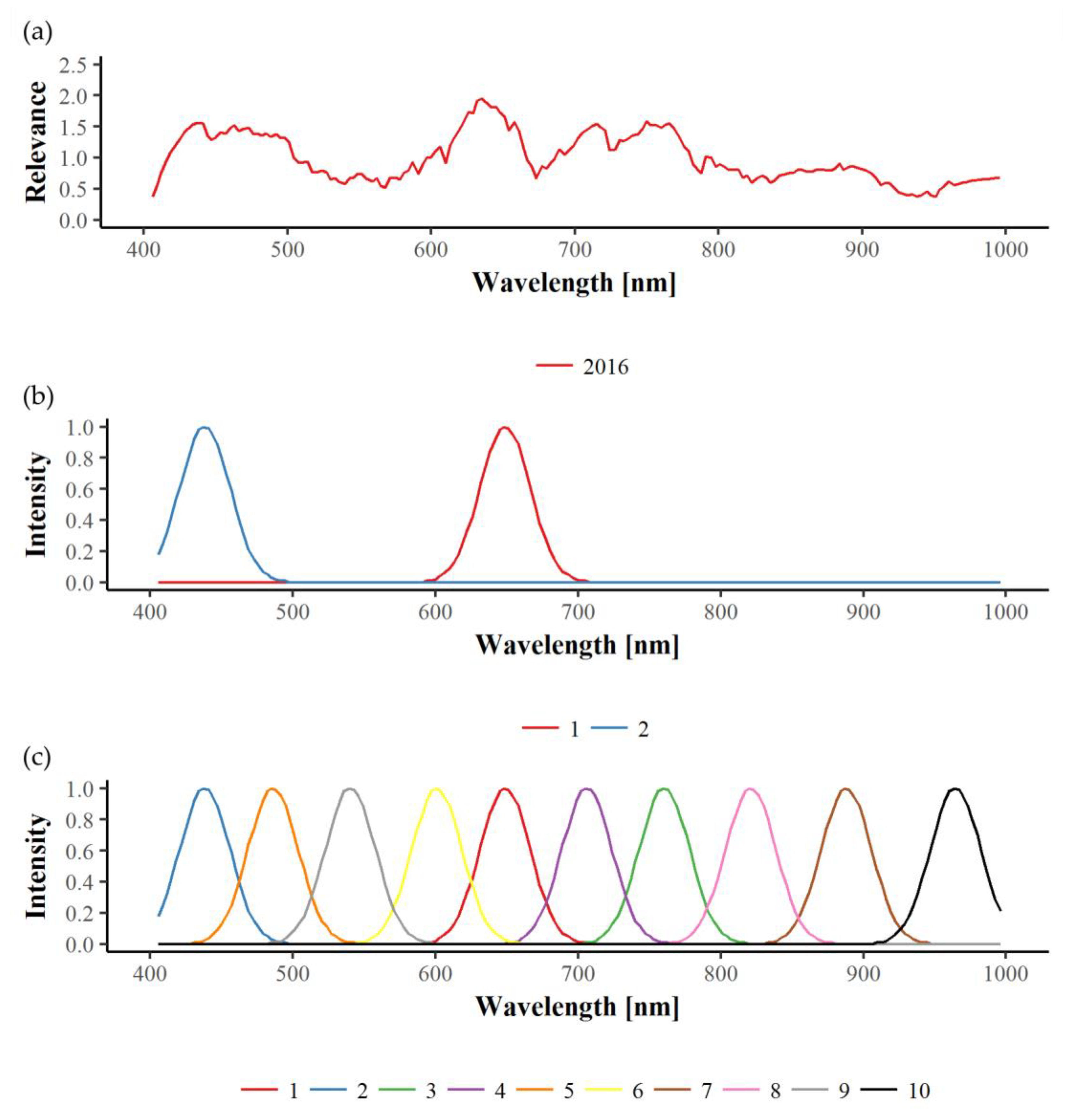
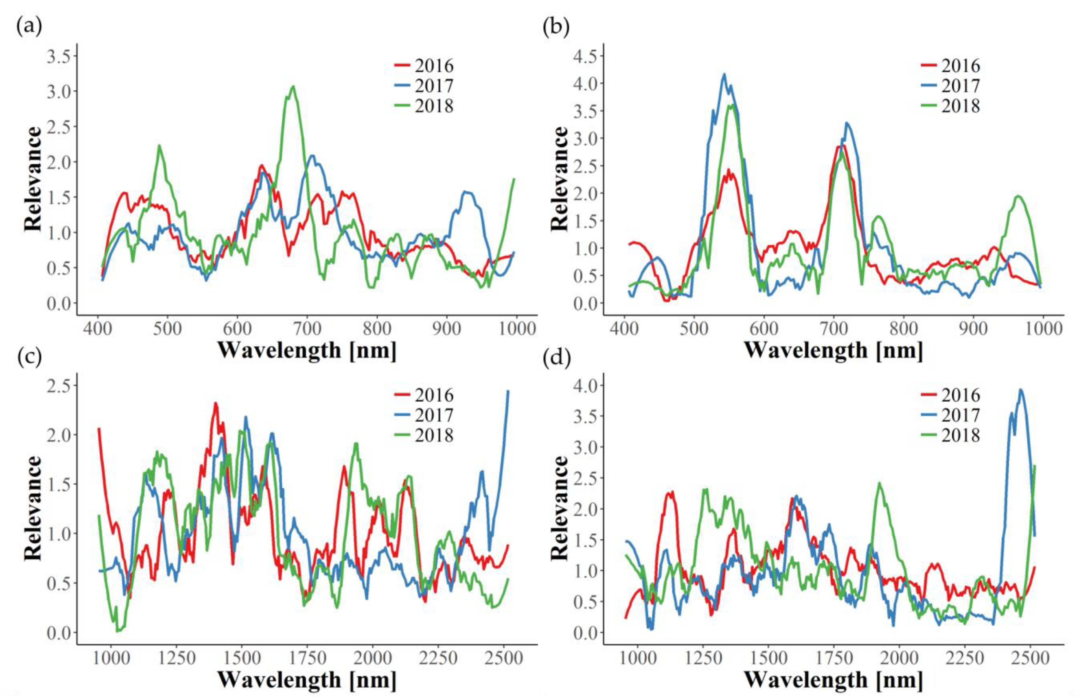
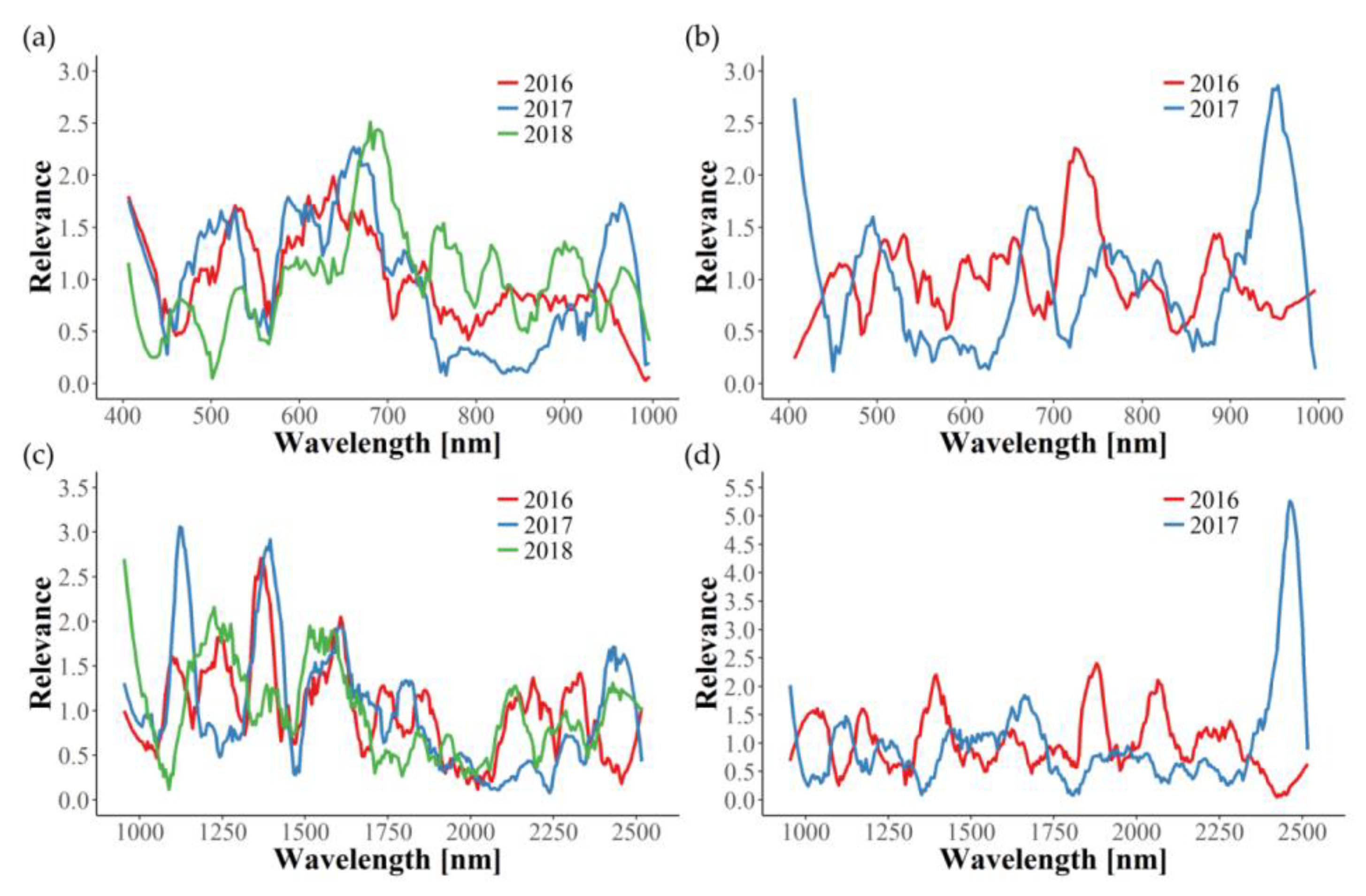
In this study, relevance profiles were calculated for the in-field disease detection, providing information about the importance of wavelengths for the differentiation tasks. In most cases, relevance profiles of the three years examined are not consistent, since many wavelengths seem to be of significance in only one or two years. Apparently, year-dependent environmental conditions interfere with the effects caused by GLD infection, thus hindering the development of one uniform disease detection model. The only exception in this work is the identification of GLRaV-1 in red cultivars using the VNIR wavelength range. Here, similar graphs can be observed for the three years, with wavelengths around 550 and 710 nm being the most important. Naidu et al. [25] also observed changes in these spectral regions for GLRaV-3 symptomatic Cabernet Sauvignon and Merlot plants. In our work, the relevance of 550 and 710 nm could also be seen for GLRaV-3 infected red cultivars in 2016, but not in 2017. Therefore, further experimental years would be helpful in determining important spectral regions of GLRaV-3 infection. Gitelson et al. [54] found that reflectance in these two spectral bands (550 ± 15 and 700 ± 7.5 nm) is well suited to estimate leaves’ anthocyanin content non-destructively and, subsequently, introduced the anthocyanin reflectance index (ARI). Thus, our findings can be clearly correlated to the increase of anthocyanin concentration in red cultivars upon GLD symptom development [47].

Through the identification of application specific wavelengths data dimensionality can be reduced and, as a consequence thereof, computational analysis and processing becomes more efficient. Using optimal spectral bands is a common approach that has successfully been implemented for the detection of three sugar beet diseases [55], anthracnose on strawberries [56], yellow rust on winter wheat [57], and powdery mildew as well as Flavescence dorée on grapevines [58,59]. Moshou et al. [57] and Yeh et al. [56] demonstrated that the number of selected spectral bands significantly influences classification, which is in accordance with our results—classification improves as more wavelengths are considered and is comparable to using the whole spectral range. This was also reported by Wang et al. [20] who identified eight wavelengths that achieved the same plant-level accuracies as the entire spectrum for the detection of tomato spotted wilt virus. Although most relevance profiles in our study vary between the three years, classification within one year is always successful when using the identified spectral bands. Al-Saddik et al. [60] developed spectral disease indices (SDIs) for the detection of Flavescence dorée, but their best wavelengths selected were different from one case to another and, therefore, no universal SDI was found to be applicable. Moreover, Sinha et al. [26] tried to transfer relevant wavelengths from one year to another for identification of GLRaV-3 in Cabernet Sauvignon vines, but results were very divergent and transfer was only partially satisfying.

However, symptom detection is only the first step in disease management. There appears to be a delay of at least one growing season between virus inoculation and symptom manifestation [61], and given the fact that some cultivars, rootstocks and most wild Vitis species do not exhibit symptoms at all [4], identification of symptomless carriers is crucial to reduce pathogen reservoirs in vineyards. GLRaVs are known to affect primary and secondary metabolism in asymptomatic plants leading to alterations in the composition of leaf biochemicals and subsequently causing changes in reflectance spectra [62,63]. The detection of asymptomatic plants was successful under greenhouse conditions even though only few plants could be used for modeling. However, in-field identification was challenging in both VNIR and SWIR for GLRaV-1 and -3, respectively. Naidu et al. [25] also used leaves from field-grown vines to detect GLRaV-3 before developing symptoms and gained significantly lower classification results (max. 75%) in comparison to symptomatic leaves. A possible explanation is that GLRaVs are unevenly distributed within grapevines and virus titer differs in the course of a growing season [64,65,66]. In contrast to field-grown grapevines, greenhouse plants consisted of only one shoot, which could lead to higher virus concentrations and better distribution, resulting in satisfying CAs. In general, detection of asymptomatic vines would not only be helpful for winegrowers in commercial vineyards but could also be a useful tool for nurseries as it might improve their ability to provide virus-free plant material to growers. Although the presented system is applicable to mother vineyards, further efforts are required to optimize classification accuracies for better in-field detection of infected, but symptomless, mother plants. Moreover, field nurseries could be screened, but here too, further improvements and a different experimental setup would be necessary as the plants are rather small and densely planted. However, young grafted plants could be analyzed after removing them from callusing boxes since most of them developed several leaves or even shoots by then [67]. Spectra of these plants could be assessed in a similar approach as was presented in this study for greenhouse plants that showed promising results with regard to asymptomatic disease detection.

5. Conclusions

Grapevine leafroll disease is considered to be the most important grapevine virus disease as it is of great economic importance for winegrowers worldwide. Currently, identification and removal of infected vines are the only in-field treatments to reduce the spread of this disease. In this context, we evaluated ground-based hyperspectral imaging (400–2500 nm) in both greenhouse and field applications for automatic disease detection. In addition to the identification of GLRaV-3, which has already been investigated in other works, this is the first study focusing also on GLRaV-1 detection. Another novelty of our study is the consideration of not only red but also white grapevine cultivars. Symptom detection was successful in the greenhouse as well as directly in the field, reaching classification accuracies of up to 100%. However, models should also be transferred to unknown plant material at different locations in order to evaluate their robustness. Although relevant wavelengths for symptom detection were not consistent over the three-year field trial, the potential of a multispectral approach is clearly shown. Further studies could use the identified bands for development of GLD specific SDIs and compare them to common reflectance indices (e.g., normalized difference vegetation index (NDVI), normalized difference red edge index (NDRE), ARI) and the whole spectral region. In general, disease detection models were developed separately for white and red cultivars as well as separately for GLRaV-1 and -3. In a comparative approach it could be shown that symptoms in white and red cultivars can be clearly distinguished. Here, further investigations are needed to evaluate if one joint detection model would be possible. Moreover, differentiation of the two viruses was successful for both white and red cultivars. Additional GLRaVs could be included in future studies to extend the detection models. Furthermore, GLD should be discriminated from other diseases or deficiencies causing similar symptoms. Besides symptom detection, identification of asymptomatic grapevines would help to reduce pathogen reservoirs in vineyards and could be a useful tool for nurseries to provide virus-free planting material. While high classification accuracies could be reached for greenhouse plants, reliable in-field detection requires further investigations. In summary, our results show the potential of hyperspectral imaging for the detection of symptomatic and asymptomatic grapevines infected with different GLRaVs and, therefore, can serve as a good basis for future studies.

References

1. Naidu, R.A.; Maree, H.J.; Burger, J.T. Grapevine leafroll disease and associated viruses: A unique pathosystem. Annu. Rev. Phytopathol. 2015, 53, 613–634. [Google Scholar] [CrossRef] [PubMed]
2. Meng, B.; Martelli, G.P.; Golino, D.A.; Fuchs, M. Grapevine Viruses: Molecular Biology, Diagnostics and Management; Springer: Cham, Switzerland, 2017; ISBN 978-3-319-57704-3. [Google Scholar] [CrossRef]
3. Dolja, V.V.; Martelli, G.P.; Meng, B. Evolutionary aspects of grapevine virology. In Grapevine Viruses: Molecular Biology, Diagnostics and Management; Springer: Cham, Switzerland, 2017; pp. 659–688. [Google Scholar] [CrossRef]
4. Naidu, R.A.; Rowhani, A.; Fuchs, M.F.; Golino, D.A.; Martelli, G.P. Grapevine leafroll: A complex viral disease affecting a high-value fruit crop. Plant Dis. 2014, 98, 1172–1195. [Google Scholar] [CrossRef] [PubMed] [Green Version]
5. Almeida, R.P.; Daane, K.M.; Bell, V.A.; Blaisdell, G.K.; Cooper, M.L.; Herrbach, E.; Pietersen, G. Ecology and management of grapevine leafroll disease. Front. Microbiol. 2013, 4, 94. [Google Scholar] [CrossRef] [PubMed] [Green Version]
6. Tsai, C.-W.; Rowhani, A.; Golino, D.A.; Daane, K.M.; Almeida, R.P. Mealybug transmission of grapevine leafroll viruses: An analysis of virus–vector specificity. Phytopathology 2010, 100, 830–834. [Google Scholar] [CrossRef] [Green Version]
7. Martelli, G.P. Directory of virus and virus-like diseases of the grapevine and their agents. J. Plant Pathol. 2014, 96, 1–136. [Google Scholar] [CrossRef]
8. Maree, H.J.; Almeida, R.P.; Bester, R.; Chooi, K.M.; Cohen, D.; Dolja, V.V.; Fuchs, M.F.; Golino, D.A.; Jooste, A.E.; Martelli, G.P.; et al. Grapevine leafroll-associated virus 3. Front. Microbiol. 2013, 4, 82. [Google Scholar] [CrossRef] [Green Version]
9. Ito, T.; Nakaune, R. Molecular characterization of a novel putative ampelovirus tentatively named grapevine leafroll-associated virus 13. Arch. Virol. 2016, 161, 2555–2559. [Google Scholar] [CrossRef] [PubMed]
10. Laimer, M.; Lemaire, O.; Herrbach, E.; Goldschmidt, V.; Minafra, A.; Bianco, P.; Wetzel, T. Resistance to viruses, phytoplasmas and their vectors in the grapevine in Europe: A review. J. Plant Pathol. 2009, 91, 7–23. [Google Scholar]
11. Blouin, A.; Chooi, K.; Cohen, D.; MacDiarmid, R. Serological methods for the detection of major grapevine viruses. In Grapevine Viruses: Molecular Biology, Diagnostics and Management; Springer: Cham, Switzerland, 2017; pp. 409–429. [Google Scholar] [CrossRef]
12. Rowhani, A.; Osman, F.; Daubert, S.; Al Rwahnih, M.; Saldarelli, P. Polymerase chain reaction methods for the detection of grapevine viruses and viroids. In Grapevine Viruses: Molecular Biology, Diagnostics and Management; Springer: Cham, Switzerland, 2017; pp. 431–450. [Google Scholar] [CrossRef]
13. Mahlein, A.K. Plant disease detection by imaging sensors—Parallels and specific demands for precision agriculture and plant phenotyping. Plant Dis. 2016, 100, 241–251. [Google Scholar] [CrossRef] [Green Version]
14. Mishra, P.; Asaari, M.S.M.; Herrero-Langreo, A.; Lohumi, S.; Diezma, B.; Scheunders, P. Close range hyperspectral imaging of plants: A review. Biosyst. Eng. 2017, 164, 49–67. [Google Scholar] [CrossRef]
15. Humplik, J.F.; Lazár, D.; Fürst, T.; Husičková, A.; Hýbl, M.; Spichal, L. Automated integrative high-throughput phenotyping of plant shoots: A case study of the cold-tolerance of pea (Pisum sativum L.). Plant Methods 2015, 11, 20. [Google Scholar] [CrossRef] [PubMed] [Green Version]
16. Blackburn, G.A. Hyperspectral remote sensing of plant pigments. J. Exp. Bot. 2007, 58, 855–867. [Google Scholar] [CrossRef] [Green Version]
17. Griffel, L.; Delparte, D.; Edwards, J. Using Support Vector Machines classification to differentiate spectral signatures of potato plants infected with Potato virus y. Comput. Electron. Agric. 2018, 153, 318–324. [Google Scholar] [CrossRef]
18. Polder, G.; Van der Heijden, G.W.A.M.; Van Doorn, J.; Baltissen, T.A.H.M.C. Automatic detection of tulip breaking virus (TBV) in tulip fields using machine vision. Biosyst. Eng. 2014, 117, 35–42. [Google Scholar] [CrossRef] [Green Version]
19. Polder, G.; Blok, P.M.; De Villiers, H.; Van der Wolf, J.M.; Kamp, J. Potato virus y detection in seed potatoes using deep learning on hyperspectral images. Front. Plant Sci. 2019, 10, 209. [Google Scholar] [CrossRef] [PubMed] [Green Version]
20. Wang, D.; Vinson, R.; Holmes, M.; Seibel, G.; Bechar, A.; Nof, S.; Tao, Y. Early detection of Tomato spotted wilt virus by hyperspectral imaging and Outlier Removal Auxiliary Classifier Generative Adversarial Nets (OR-AC-GAN). Sci. Rep. 2019, 9, 4377. [Google Scholar] [CrossRef]
21. Chávez, P.; Zorogastúa, P.; Chuquillanqui, C.; Salazar, L.; Mares, V.; Quiroz, R. Assessing Potato yellow vein virus (PYVV) infection using remotely sensed data. Int. J. Pest Manag. 2009, 55, 251–256. [Google Scholar] [CrossRef]
22. Lee, H.; Kim, M.S.; Lim, H.-S.; Park, E.; Lee, W.-H.; Cho, B.-K. Detection of cucumber green mottle mosaic virus-infected watermelon seeds using a near-infrared (NIR) hyperspectral imaging system: Application to seeds of the “Sambok Honey” cultivar. Biosyst. Eng. 2016, 148, 138–147. [Google Scholar] [CrossRef]
23. Lu, J.; Zhou, M.; Gao, Y.; Jiang, H. Using hyperspectral imaging to discriminate yellow leaf curl disease in tomato leaves. Precis. Agric. 2018, 19, 379–394. [Google Scholar] [CrossRef]
24. Afonso, A.M.; Guerra, R.; Cavaco, A.M.; Pinto, P.; Andrade, A.; Duarte, A.; Power, D.M.; Marques, N.T. Identification of asymptomatic plants infected with Citrus tristeza virus from a time series of leaf spectral characteristics. Comput. Electron. Agric. 2017, 141, 340–350. [Google Scholar] [CrossRef]
25. Naidu, R.A.; Perry, E.M.; Pierce, F.J.; Mekuria, T. The potential of spectral reflectance technique for the detection of Grapevine leafroll-associated virus-3 in two red-berried wine grape cultivars. Comput. Electron. Agric. 2009, 66, 38–45. [Google Scholar] [CrossRef]
26. Sinha, R.; Khot, L.R.; Rathnayake, A.P.; Gao, Z.; Naidu, R.A. Visible-near infrared spectroradiometry-based detection of Grapevine leafroll-associated virus 3 in a red-fruited wine grape cultivar. Comput. Electron. Agric. 2019, 162, 165–173. [Google Scholar] [CrossRef]
27. Pagay, V.; Habili, N.; Wu, Q.; Coleman, D. Rapid and non-destructive detection of Shiraz disease and grapevine leafroll disease on asymptomatic grapevines in Australian vineyards. In Proceedings of the 19th Congress of ICVG, Santiago, Chile, 9–12 April 2018; pp. 34–35. [Google Scholar]
28. Hou, J.; Li, L.; He, J. Detection of grapevine leafroll disease based on 11-index imagery and ant colony clustering algorithm. Precis. Agric. 2016, 17, 488–505. [Google Scholar] [CrossRef]
29. MacDonald, S.L.; Staid, M.; Staid, M.; Cooper, M.L. Remote hyperspectral imaging of Grapevine leafroll-associated virus 3 in Cabernet Sauvignon vineyards. Comput. Electron. Agric. 2016, 130, 109–117. [Google Scholar] [CrossRef] [Green Version]
30. Agrarmeteorologie Rheinland-Pfalz. Available online: https://www.am.rlp.de/Internet/AM/NotesAM.nsf/amweb/752dce127578072cc12572eb0020c16c?OpenDocument (accessed on 16 May 2020).
31. Steinmetz, N.; Michl, G.; Maixner, M.; Hoffmann, C. A rapid and inexpensive RNA-extraction method for high-throughput virus detection in grapevine. Vitis 2020, 59, 35–39. [Google Scholar] [CrossRef]
32. Gambino, G.; Gribaudo, I. Simultaneous detection of nine grapevine viruses by multiplex reverse transcription-polymerase chain reaction with coamplification of a plant RNA as internal control. Phytopathology 2006, 96, 1223–1229. [Google Scholar] [CrossRef] [Green Version]
33. Beuve, M.; Moury, B.; Spilmont, A.-S.; Sempé-Ignatovic, L.; Hemmer, C.; Lemaire, O. Viral sanitary status of declining grapevine Syrah clones and genetic diversity of Grapevine Rupestris stem pitting-associated virus. Eur. J. Plant Pathol. 2013, 135, 439–452. [Google Scholar] [CrossRef]
34. Ochoa-Corona, F.M.; Lebas, B.M.S.; Tang, J.; Stewart, F.J.; Elliott, D.R.; Alexander, B.J.R. Diagnosis and strain typing of Pepino mosaic virus and Raspberry ringspot virus by RT-PCR and SSCP. In Proceedings of the 15th Biennial Australasian Plant Pathology Society Conference, Geelong, VIC, Australia, 26–29 September 2005; Conference Handbook. p. 259. [Google Scholar]
35. Kicherer, A.; Herzog, K.; Bendel, N.; Klück, H.C.; Backhaus, A.; Wieland, M.; Rose, J.C.; Klingbeil, L.; Läbe, T.; Hohl, C.; et al. Phenoliner: A new field phenotyping platform for grapevine research. Sensors 2017, 17, 1625. [Google Scholar] [CrossRef]
36. Cybenko, G. Approximation by superpositions of a sigmoidal function. Math. Control Signals Syst. 1989, 2, 303–314. [Google Scholar] [CrossRef]
37. Asaari, M.S.M.; Mishra, P.; Mertens, S.; Dhondt, S.; Inzé, D.; Wuyts, N.; Scheunders, P. Close-range hyperspectral image analysis for the early detection of stress responses in individual plants in a high-throughput phenotyping platform. ISPRS J. Photogram. Remote Sens. 2018, 138, 121–138. [Google Scholar] [CrossRef]
38. Krzanowski, W. Principles of Multivariate Analysis: A User’s Perspective; Clarendon Press: Oxford, UK, 1988; pp. 291–301. [Google Scholar]
39. Wold, S.; Sjöström, M.; Eriksson, L. PLS-regression: A basic tool of chemometrics. Chemom. Intell. Lab. Syst. 2001, 58, 109–130. [Google Scholar] [CrossRef]
40. Møller, M.F. A scaled conjugate gradient algorithm for fast supervised learning. Neural Netw. 1993, 6, 525–533. [Google Scholar] [CrossRef]
41. Moody, J.; Darken, C.J. Fast learning in networks of locally-tuned processing units. Neural Comput. 1989, 1, 281–294. [Google Scholar] [CrossRef]
42. Backhaus, A.; Bollenbeck, F.; Seiffert, U. Robust classification of the nutrition state in crop plants by hyperspectral imaging and artificial neural networks. In Proceedings of the 2011 3rd Workshop on Hyperspectral Image and Signal Processing: Evolution in Remote Sensing (Whispers), Lisbon, Portugal, 6–9 June 2011; pp. 1–4. [Google Scholar] [CrossRef]
43. Dehghani, R.; Mahdavi-Amiri, N. Scaled nonlinear conjugate gradient methods for nonlinear least squares problems. Numer. Algorithms 2019, 82, 1–20. [Google Scholar] [CrossRef]
44. Martinetz, T.M.; Berkovich, S.G.; Schulten, K.J. ‘Neural-gas’ network for vector quantization and its application to time-series prediction. IEEE Transact. Neural Netw. 1993, 4, 558–569. [Google Scholar] [CrossRef]
45. Gutiérrez, S.; Fernandez-Novales, J.; Diago, M.P.; Tardaguila, J. On-the-go hyperspectral imaging under field conditions and machine learning for the classification of grapevine varieties. Front. Plant Sci. 2018, 9, 1102. [Google Scholar] [CrossRef]
46. Albetis, J.; Duthoit, S.; Guttler, F.; Jacquin, A.; Goulard, M.; Poilvé, H.; Féret, J.-B.; Dedieu, G. Detection of Flavescence dorée grapevine disease using Unmanned Aerial Vehicle (UAV) multispectral imagery. Remote Sens. 2017, 9, 308. [Google Scholar] [CrossRef] [Green Version]
47. Gutha, L.R.; Casassa, L.F.; Harbertson, J.F.; Naidu, R.A. Modulation of flavonoid biosynthetic pathway genes and anthocyanins due to virus infection in grapevine (Vitis vinifera L.) leaves. BMC Plant Biol. 2010, 10, 187. [Google Scholar] [CrossRef] [Green Version]
48. Walker, A.R.; Lee, E.; Bogs, J.; McDavid, D.A.; Thomas, M.R.; Robinson, S.P. White grapes arose through the mutation of two similar and adjacent regulatory genes. Plant J. 2007, 49, 772–785. [Google Scholar] [CrossRef]
49. Al-Saddik, H.; Simon, J.-C.; Cointault, F. Assessment of the optimal spectral bands for designing a sensor for vineyard disease detection: The case of ‘Flavescence dorée’. Precis. Agric. 2019, 20, 398–422. [Google Scholar] [CrossRef]
50. Berdugo, C.; Zito, R.; Paulus, S.; Mahlein, A.K. Fusion of sensor data for the detection and differentiation of plant diseases in cucumber. Plant Pathol. 2014, 63, 1344–1356. [Google Scholar] [CrossRef]
51. Fan, X.; Hong, N.; Dong, Y.; Ma, Y.; Zhang, Z.P.; Ren, F.; Hu, G.; Zhou, J.; Wang, G. Genetic diversity and recombination analysis of Grapevine leafroll-associated virus 1 from China. Arch. Virol. 2015, 160, 1669–1678. [Google Scholar] [CrossRef] [PubMed]
52. Maree, H.J.; Pirie, M.D.; Oosthuizen, K.; Bester, R.; Rees, D.J.G.; Burger, J.T. Phylogenomic analysis reveals deep divergence and recombination in an economically important grapevine virus. PLoS ONE 2015, 10. [Google Scholar] [CrossRef] [PubMed]
53. Angelini, E.; Aboughanem-Sabanadzovic, N.; Dolja, V.V.; Meng, B. Grapevine leafroll-associated virus 2. In Grapevine Viruses: Molecular Biology, Diagnostics and Management; Springer: Cham, Switzerland, 2017; pp. 141–165. [Google Scholar] [CrossRef]
54. Gitelson, A.A.; Merzlyak, M.N.; Chivkunova, O.B. Optical properties and nondestructive estimation of anthocyanin content in plant leaves. Photochem. Photobiol. 2001, 74, 38–45. [Google Scholar] [CrossRef]
55. Mahlein, A.K.; Rumpf, T.; Welke, P.; Dehne, H.W.; Plümer, L.; Steiner, U.; Oerke, E.C. Development of spectral indices for detecting and identifying plant diseases. Remote Sens. Environ. 2013, 128, 21–30. [Google Scholar] [CrossRef]
56. Yeh, Y.-H.; Chung, W.-C.; Liao, J.-Y.; Chung, C.-L.; Kuo, Y.-F.; Lin, T.-T. Strawberry foliar anthracnose assessment by hyperspectral imaging. Comput. Electron. Agric. 2016, 122, 1–9. [Google Scholar] [CrossRef]
57. Moshou, D.; Bravo, C.; Wahlen, S.; West, J.; McCartney, A.; De Baerdemaeker, J.; Ramon, H. Simultaneous identification of plant stresses and diseases in arable crops using proximal optical sensing and self-organising maps. Precis. Agric. 2006, 7, 149–164. [Google Scholar] [CrossRef]
58. Knauer, U.; Matros, A.; Petrovic, T.; Zanker, T.; Scott, E.S.; Seiffert, U. Improved classification accuracy of powdery mildew infection levels of wine grapes by spatial-spectral analysis of hyperspectral images. Plant Methods 2017, 13, 47. [Google Scholar] [CrossRef]
59. Al-Saddik, H.; Laybros, A.; Billiot, B.; Cointault, F. Using image texture and spectral reflectance analysis to detect Yellowness and Esca in grapevines at leaf-level. Remote Sens. 2018, 10, 618. [Google Scholar] [CrossRef] [Green Version]
60. Al-Saddik, H.; Simon, J.C.; Cointault, F. Development of spectral disease indices for ‘Flavescence Doree’ grapevine disease identification. Sensors 2017, 17, 2772. [Google Scholar] [CrossRef] [Green Version]
61. Blaisdell, G.K.; Cooper, M.L.; Kuhn, E.J.; Taylor, K.A.; Daane, K.M.; Almeida, R.P.P. Disease progression of vector-mediated Grapevine leafroll-associated virus 3 infection of mature plants under commercial vineyard conditions. Eur. J. Plant Pathol. 2016, 146, 105–116. [Google Scholar] [CrossRef] [Green Version]
62. Montero, R.; Pérez-Bueno, M.L.; Barón, M.; Florez-Sarasa, I.; Tohge, T.; Fernie, A.R.; El Aou Ouad, H.; Flexas, J.; Bota, J. Alterations in primary and secondary metabolism in Vitis vinifera ‘Malvasía de Banyalbufar’upon infection with Grapevine leafroll-associated virus 3. Physiol. Plant 2016, 157, 442–452. [Google Scholar] [CrossRef] [PubMed]
63. Bertamini, M.; Muthuchelian, K.; Nedunchezhian, N. Effect of grapevine leafroll on the photosynthesis of field grown grapevine plants (Vitis vinifera L. cv. Lagrein). J. Phytopathol. 2004, 152, 145–152. [Google Scholar] [CrossRef]
64. Tsai, C.; Daugherty, M.; Almeida, R. Seasonal dynamics and virus translocation of Grapevine leafroll-associated virus 3 in grapevine cultivars. Plant Pathol. 2012, 61, 977–985. [Google Scholar] [CrossRef]
65. Osman, F.; Golino, D.; Hodzic, E.; Rowhani, A. Virus distribution and seasonal changes of Grapevine leafroll-associated viruses. Am. J. Enol. Vitic. 2018, 69, 70–76. [Google Scholar] [CrossRef]
66. Chooi, K.M.; Cohen, D.; Pearson, M.N. Differential distribution and titre of selected Grapevine leafroll-associated virus 3 genetic variants within grapevine rootstocks. Arch. Virol. 2016, 161, 1371–1375. [Google Scholar] [CrossRef]
67. Gramaje, D.; Armengol, J. Fungal trunk pathogens in the grapevine propagation process: Potential inoculums sources, detection, identification, and management strategies. Plant Dis. 2011, 95, 1040–1055. [Google Scholar] [CrossRef] [Green Version]
Figure 1. Overview of the workflow for field data of control (left) and grapevine leafroll-associated viruses (GLRaV-1) infected (right) vines. Depicted are a calibrated reflectance image at 800 nm coded as grey scale (a,b) and an RGB reconstruction (red-green-blue color space) (c,d), which is for visualization only. The hyperspectral image was segmented into leaves, grapes, stem material, and background (e,f) and detection models were applied on leaf pixels only (g,h). Vines were labeled with their GPS position and a 50 cm wide window was placed around each of them to avoid overlaps between plants. Based on a majority vote of pixel results per window the whole vine was classified as infected or healthy (i,j).
Remotesensing 12 01693 g001
Figure 2. Overview of the workflow for greenhouse data of control (left) and GLRaV-1 infected (right) vines. Depicted are a calibrated reflectance image at 800 nm coded as grey scale (a,b) and an RGB reconstruction (c,d), which is for visualization only. The hyperspectral image was segmented into its main components and the binary classifier detecting GLRaV-1 was applied to leaf pixels calculating the ratio of symptomatic pixels to all available pixels, thereby, classifying the whole plant as infected or healthy (e,f).
Remotesensing 12 01693 g002
Figure 3. Example of the band selection process in the VNIR range for GLRaV-1 symptom detection of white cultivars in 2016. According to the relevance profile (a), multispectral bands can be selected starting with the two most informative. (b) Single bands can be added until a maximum of ten is reached (c).
Remotesensing 12 01693 g003
Figure 4. Spectral relevance profiles for VNIR (a,b) and SWIR (c,d) in three consecutive years regarding white (a,c) and red (b,d) cultivars infected with GLRaV-1.
Remotesensing 12 01693 g004