Modeling and Analysis of an Echo Laser Pulse Waveform for the Orientation Determination of Space Debris

Abstract

Orientation information of space debris is required to improve the orbital prediction accuracy for mitigation or elimination of a significant threat to not only human space activities but also operational satellites. Obtaining orientation information is currently achievable by applying photometry, adaptive optics (AO) and satellite laser ranging (SLR) technologies. In this study, a new method is proposed based on an echo laser pulse waveform (ELPW) for the orientation determination of space debris; its feasibility was also investigated by numerical simulations. Unlike the photometry and AO technologies available just under the sun-illumination condition and the SLR technology applicable only for cooperative targets, the ELPW is achievable by using a high power laser regardless of the above measurement constraints. A mathematical model is derived to generate the ELPW, and the beam broadening and spreading due to the atmospheric turbulence is taken into account. The Gaussian decomposition based on a genetic algorithm was employed to the ELPWs in order to analyze the orientation features. It is demonstrated from the numerical simulations that the ELPWs have distinctive shapes characterizing the orientation of space debris and therefore our approach was capable of providing orientation information.

1. Introduction

Space debris has become an important global problem because the exponential growth of its population poses a significant threat to not only human space activities but also operational satellites. Improving the orbital prediction accuracy of space debris is required to mitigate or eliminate the threat through avoidance of catastrophic collisions, which is attainable by using various measurements from the optical, radar and laser tracking systems. Even though these tracking systems provide accurate measurements, the dynamic model has to take into consideration the space debris characteristics such as size, shape and orientation information in order to improve the orbital prediction accuracy. Unlike the gravitational perturbations, non-gravitational perturbations such as the atmospheric drag and solar radiation pressure are dominated by these characteristics [1]. Thus the orientation determination including rotation rates and axis of space debris became a topic of interest in the space situational awareness communities.

There are several methods to achieve orientation information of space debris in terms of the ground-based observations: photometry, adaptive optics (AO) and satellite laser ranging (SLR). Photometry is literally the measurement of light intensity or brightness and provides light curves which are commonly used in the astronomical communities to extract physical information of asteroids. Recently light curves have been recognized as a promising tool to determine shapes, spin axis orientation and spin rate of space debris by analyzing amplitude variation as well as periodic difference, thus are widely used by many researchers [2,3,4,5,6,7]. The AO is a technology to improve the image quality nearly to diffraction limited resolution by compensating the incoming wavefronts distorted by the atmospheric turbulence. So the high-resolution optical images obtained from the AO system provide a means of characterizing size, shape and orientation of space debris and its identification [8,9,10].

As opposed to the passive technologies (i.e., photometry and AO) which receive sunlight reflected by space debris and so work only at night (in particular, twilight for space debris in low earth orbit), the SLR technology actively fires laser pulses into space objects and then measures the distance between the ground station and space objects equipped with corner cube reflectors (CCRs). The spinning array of the CCRs causes a millimeter-scale distance variation from which information of spin axis orientation and spin rate is achievable [11] for not only geodetic satellites with CCRs on the outer surface [12,13,14] but also defunct satellites equipped with CCRs [15,16,17]. Moreover, the SLR technology combined with photometry has been applied to space debris without CCRs, called uncooperative targets [18,19,20].

Debris laser ranging (DLR) is similar to SLR but applicable to uncooperative targets by employing a higher power laser rather than the SLR (normally 2 or 3 orders of power). It generates ranging data even under the low signal-to-noise ratio resulting from a small laser cross-section of uncooperative targets. For DLR, a Geiger-mode avalanche photodiode, called a photon-counting detector, is applied to respond to the presence of return signals and then records accurate timing of the first arrived photon [21,22,23,24]. In spite of benefits from the photon-counting detector with higher detection sensitivity and lower dark noise, it does not provide an echo laser pulse waveform (ELPW) which records the scattering signals as a function of time. The ELPWs are achievable for uncooperative targets by employing a linear-mode avalanche photodiode (LmAPD) and a much higher power laser on the DLR system because the LmAPD output current is linearly proportional to photocurrent and thus can provide intensity information as well as ranging measurements. An ELPW allows not only range information but also 3-D shape in the direction of laser beam propagation by analyzing the features of the scattering signals, without an optical scanning system [25].

In this study, a new method based on the ELPW analysis was proposed for orientation determination of space debris and its feasibility was also investigated by numerical simulations of two space targets (i.e., defunct satellite and rocket body). Unlike the passive and SLR technologies, the proposed method is free of the measurement constraints such as sun-illumination and CCRs requirement. Approximating that the reflected surface of a space target consists of small grids, a mathematical model was derived to generate the ELPW for the fully reflected surface, which takes into consideration temporal beam broadening and spatial beam spreading due to the atmospheric turbulence. The simulation took into account detector noise and amplifier noise by assuming that the noises are independent and of Gaussian distribution in the optical power domain. A genetic algorithm was also introduced to determine the Gaussian parameters of Gaussian decomposition and to analyze the relationship between ELPW features and orientation of the space target in terms of Gaussian parameters. It was shown from the numerical simulations that the proposed method was a feasible alternative to achieve orientation information because the ELPW had a distinctive shape characterizing the orientation of space debris.

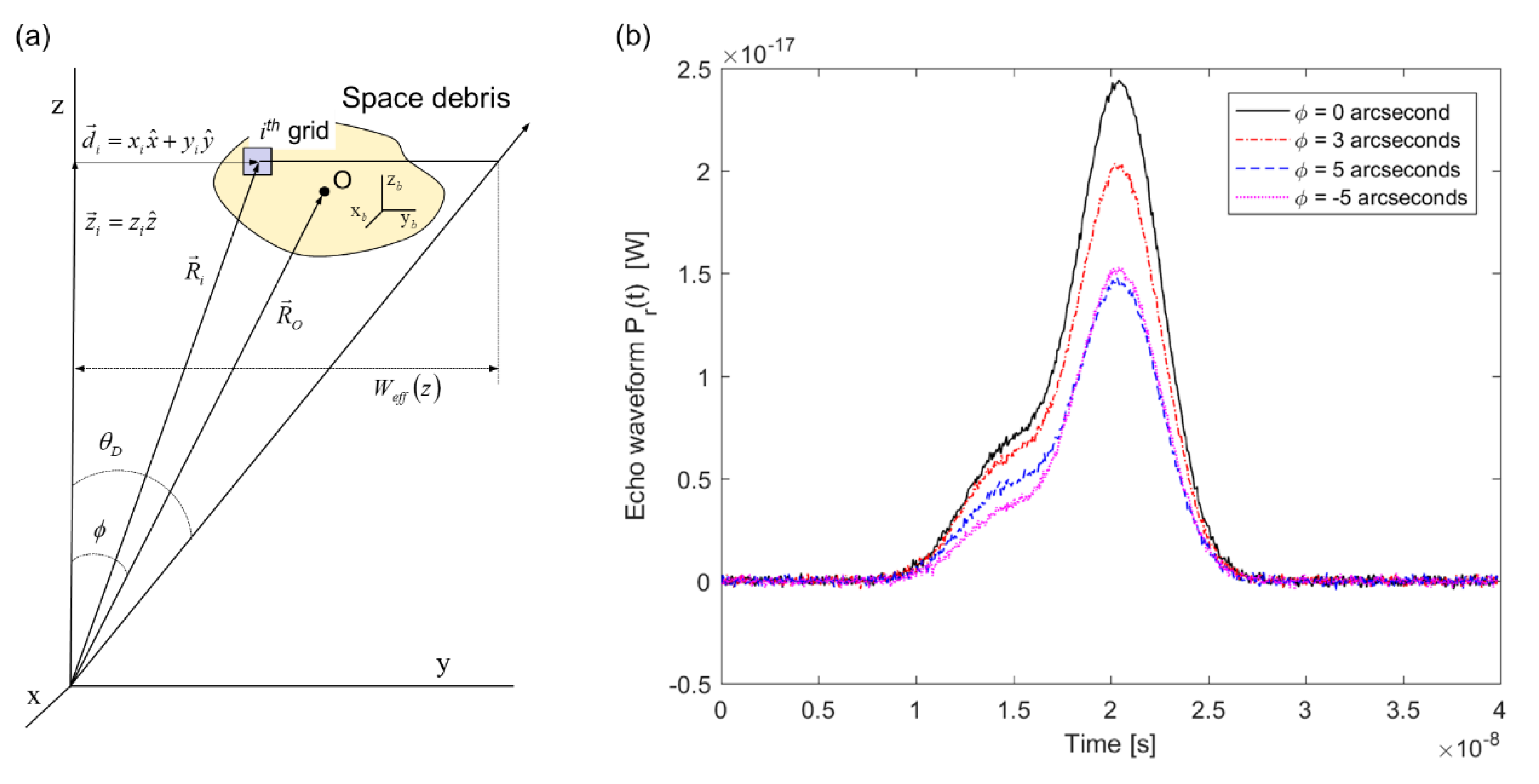
2. Mathematical Model

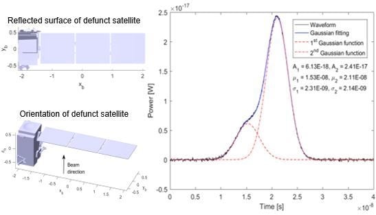
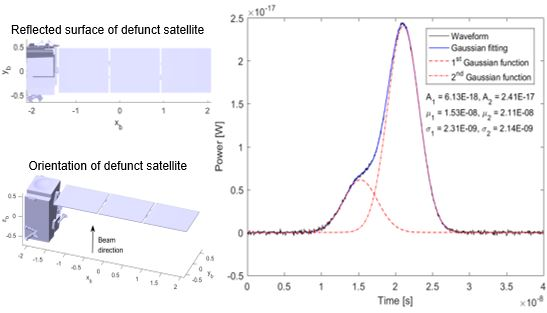
2.1. Echo Laser Pulse Waveform

The intensity of a laser beam is not uniform in temporal and spatial domains along the direction of laser beam propagation, which requires that the laser pulse profile should be modeled in time as well as in space. The laser beam propagation can be approximated by assuming that the laser beam has a Gaussian shape in terms of temporal and spatial domains. So the irradiance distribution and normalized waveform of the propagated laser pulse are expressed as [26,27]

$$I\left(d,z\right)=\frac{2P_T}{\pi W_{eff}^2\left(z\right)}\exp \left[-2\frac{d^2}{W_{eff}^2\left(z\right)}\right],$$

(1)

$$p\left(t\right)=\frac{1}{\sqrt{2\pi }{\tau }_0}\exp \left[-\frac{t^2}{2{\tau }_0^2}\right],$$

(2)

where $d$ is the radial distance from the axis of propagation (i.e., $d^2=x^2+y^2$), $z$ is the axial distance from the beam’s narrowest point called waist, $P_T$ is the transmitted power, $W_{eff}\left(z\right)$ is the effective beam size referred to as the Gaussian beam radius, and ${\tau }_0$ is the transmitted pulse width which is related to the full width at half maximum (FWHM) as follows: $FWHM=2\sqrt{2\ln 2}{\tau }_0$ [28].

The reflected or intersected surface of space debris by the laser beam is assumed to consist of small grids in order to generate a total ELPW. Some of the laser power received by the ith grid located at $\left(x_i,y_i\right)$ is absorbed while the rest is reradiated back into space, in proportion to the effective receiving area depending on the incident angle ${\theta }_i$. Therefore the scattered power by the ith grid is described by

$$P_{S,i}=\frac{2P_T}{\pi W_{eff}^2\left(z_i\right)}\exp \left[-2\frac{d_i^2}{W_{eff}^2\left(z_i\right)}\right]\cdot \left(\rho A_i\cos {\theta }_i\right),$$

(3)

where $A_i$ is the ith grid area, and $\rho$ is the reflectivity on the assumption that all grids have the same reflectivity in this study. Large grid areas can save computation time but might provide ELPW features less accurate from the true orientation of space target. So all grids should have optimal areas so that the ELPW simulation closely resembles a practical situation with minimal computation time, smaller than 50 cm² in this study. If the incoming radiation to the receiver is scattered uniformly into a cone of solid angle $\mathsf{\Omega }$ [29], the laser power coming into the receiver (i.e., received power) is given by

$$P_{R,i}=\frac{2P_T}{\pi W_{eff}^2\left(z_i\right)}\exp \left[-2\frac{d_i^2}{W_{eff}^2\left(z_i\right)}\right]\cdot \left(\rho A_i\cos {\theta }_i\right)\cdot \frac{A_R}{\Omega R_i^2},$$

(4)

where $A_R$ is the receiving area, and $R_i$ is the range to the ith grid. The solid angle can be replaced with $\pi$ by considering the grid to be a diffuse scattering target, or a Lambertian target. Taking into consideration the normalized waveform given by Equation (2), the received power in terms of the time domain can be written by

$$P_{R,i}\left(t\right)=\frac{P_T}{\pi R_i^2}{G}_i\left(t\right)\rho A_i\cos {\theta }_i{A}_R,$$

(5)

$$G_i\left(t\right)=\frac{2}{\pi W_{eff}^2\left(z\right)}\exp \left[-2\frac{d_i^2}{W_{eff}^2\left(z\right)}\right]\cdot \frac{1}{\sqrt{2\pi }{\tau }_R}\exp \left[-\frac{1}{2{\tau }_R^2}{\left(t-\frac{2R_i}{c}\right)}^2\right],$$

(6)

where $c$ is the light speed in a vacuum, and ${\tau }_R$ is the received pulse width, which is broadened by the atmospheric turbulence. The echo waveform model was also given by Hao et al. [30] for the case of specular targets such as mirrors, which increases significantly the received power compared to diffuse targets. Space debris and most satellites are considered as diffuse targets since they are non-cooperative targets without CCRs and the echo signals are diffused from their surface.

In the practical DLR system, the transmitted laser beam suffers from various attenuations by the time it comes back to a detector, e.g., atmospheric attenuation, and optical transmittance. Taking into account various attenuations in Equation (5), the mathematical equation of ELPW is obtained by summing the received power corresponding to a grid as follows:

$$P_r\left(t\right)={\displaystyle \sum _{i=1}^N\frac{P_t}{\pi R_i^2}{G}_i\left(t\right)\rho \cos {\theta }_i{A}_i{A}_R{T}_A^2{T}_C^2{\eta }_T{\eta }_R{\eta }_F},$$

(7)

where $N$ is the total number of grids illuminated by the transmitted laser beam, $T_A$ and $T_C$ are the one-way transmittance by the atmospheric attenuation and cirrus clouds, respectively, ${\eta }_T$ is the transmitting optical efficiency, ${\eta }_R$ is the receiving optical efficiency, and ${\eta }_F$ is the optical filter transmittance.

In the near-ultraviolet to visible spectral band (0.3~0.7 μm), the atmospheric attenuation is dominated by aerosol and molecular scattering as well as ozone absorption. In the near infrared band beyond 0.7 μm, attenuation is subjected to absorption features of atmospheric constituents including water vapor, oxygen and carbon dioxide. Typically, cirrus clouds are overhead about 50% of the time at most locations. The one-way transmittances by the atmospheric attenuation and cirrus clouds are expressed as [31]

$$T_A\left(\lambda ,V,h_s\right)=\exp \left[-\sigma \left(\lambda ,V,0\right)h_{SH}\sec \left({\theta }_Z\right)\exp \left(-\frac{h_s}{h_{SH}}\right)\right],$$

(8)

$$T_C=\exp \left[-0.14{\left(C_T\sec {\theta }_z\right)}^2\right],$$

(9)

where $\sigma \left(\lambda ,V,0\right)$ and $V$ are the atmospheric attenuation coefficient and the visibility at sea level, respectively, $\lambda$ is the laser beam wavelength, $h_{SH}$ is the scale height of 1.2 km, ${\theta }_Z$ is the zenith angle of space target, $h_s$ is the station height, and $C_T$ is the cirrus cloud thickness.

2.2. Laser Beam Spreading and Broadening

When the laser beam propagates through the atmosphere, the atmospheric refractive index is randomly fluctuated due to the atmospheric turbulence, resulting in the intensity fluctuations known as scintillation, phase distortion, beam spot wandering, beam spreading and broadening. In particular, the spatial spreading and temporal broadening of laser beams are limiting factors in most applications such as remote sensing and free space optical communications [32]. The effective beam size of a Gaussian beam in a horizontal path is approximated in a far-field region as follows [33]:

$$W_{eff}^2\left(z\right)=W^2\left(z\right)\left(1+T\right),$$

(10)

where:

$$W\left(z\right)=W_0\sqrt{1+{\left(\frac{2z}{k{W}_0^2}\right)}^2}\approx \frac{2z}{k{W}_0^2}=z{\theta }_D,$$

(11)

$$T=4.35k^{7/6}{\left(\Lambda H\right)}^{5/6}{\sec }^{11/6}\left({\theta }_z\right){\displaystyle {\int }_{h_s}^{h_s+H}{C}_n^2\left(h\right){\left(1-\frac{h-h_s}{H}\right)}^{5/3}}dh,$$

(12)

where $T$ is the additional parameter corresponding to the beam spreading by the atmospheric turbulence, $k$ is the optical wavenumber, $W_0$ is the beam size at $z=0$ (called beam waist), ${\theta }_D$ is the far-field divergence half-angle, $\mathsf{\Lambda }$ is the Fresnel ratio defined as $\Lambda =2z/k{W}^2\left(z\right)$, $H$ is the space debris altitude from the station, and $C_n^2\left(h\right)$ is the refractive-index structure parameter which represents the intensity of atmospheric turbulence.

Many models have been proposed to predict the behavior of the refractive-index structure parameter. The Hufnagel-Valley model is widely used in satellite optical communications and optical remote sensing because it allows easy variation of day-time and night-time profile by varying various site parameters such as wind speed, isoplanatic angle and altitude [34]. The model is given by

$$C_n^2\left(h\right)=0.00594{\left(\frac{v}{27}\right)}^2{\left({10}^{-5}h\right)}^{10}\exp \left(-\frac{h}{1000}\right)+2.7\times {10}^{-16}\exp \left(-\frac{h}{1500}\right)+A_0\exp \left(-\frac{h}{100}\right),$$

(13)

where $v$ is the mean square value of the wind speed in $m/s$, and $A_0$ is the nominal value of the refractive-index structure parameter at the ground in $m^{-2/3}$.

The temporal broadening of a laser pulse through the atmosphere is caused physically by two mechanisms: scattering process and beam spot wandering; these are too important to be neglected for high bandwidth signals such as narrow pulses in the range from femtosecond to picosecond [35]. The received pulse width broadened by the atmospheric turbulence is given by [32]

$${\tau }_R=\sqrt{{\tau }_0^2+8\chi },$$

(14)

where:

$$\chi =0.391\left(1+0.171{\beta }^2-0.287{\beta }^{5/3}\right)\mu \sec {\theta }_z/c^2,$$

(15)

$$\mu ={\displaystyle {\int }_{h_s}^{h_s+H}{C}_n^2\left(h\right){\left[L_0\left(h\right)\right]}^{5/3}}dh,$$

(16)

$$L_0\left(h\right)=5{\left[1+{\left(\frac{h-7500}{2500}\right)}^2\right]}^{-1},l_0\left(h\right)=\beta L_0\left(h\right),$$

(17)

where $\beta$ is the inner scale factor, $0<\beta <1$, and $l_0\left(h\right)$ and $L_0\left(h\right)$ represent the inner and outer scale sizes as a function of altitude, respectively.

2.3. Noise Equivalent Power

The received signal is subject to amplifier and detector noises including background noise, shot noise and dark current noise, all of which should be considered in the ELPW simulation. The noise equivalent power (NEP) is a common metric that quantifies the sensitivity of a photodetector or the power generated by a noise source, which means the minimum optical power required to achieve a unity signal-to-noise ratio in a 1 Hz bandwidth. To take into account noise in the ELPW simulation, a Gaussian random variable with a zero mean and a standard deviation equal to NEP is generated and then added to the received power because the noises are independent and identically distributed Gaussian random variables [36]. The NEP resulting from the detector noise is given by

$$NE{P}_{Detector}\left(t\right)=\frac{\sqrt{2qB\left[I_{ds}+\left(I_{db}+I_b+I_s\right)G^2{F}_A\right]}}{\Re },$$

(18)

where $q$ is the electronic charge, $B$ is the electrical bandwidth, $I_{ds}$ and $I_{db}$ are the surface and bulk dark currents, respectively, $I_b$ and $I_s$ are the currents due to the background noise and received signal, respectively, $G$ is the detector gain, $F_A$ is the excess noise factor, $\Re$ is the detector responsivity defined as $\Re =q{\eta }_{Q}G/hv$ using the quantum efficiency of the detector ${\eta }_Q$, h is Plank’s constant and the laser beam frequency is $v$. The excess noise factor is expressed as $F_A=k_{eff}G+\left(1-k_{eff}\right)\left(2-1/G\right)$ in terms of the detector gain and the ionization coefficient ratio $k_{eff}$. Two currents owing to the received signal and background noise in Equation (18) can be obtained from [37]

$$I_s\left(t\right)=\Re P_r\left(t\right),$$

(19)

$$I_b=\Re P_b=I_{\lambda }{\Omega }_{FoV}{\eta }_R{\eta }_F{A}_R\Delta {\lambda }_F,$$

(20)

where $I_{\lambda }$ is the spectral radiance of the sky, ${\Omega }_{FoV}$ is the receiver field of view in steradians, and $\Delta {\lambda }_F$ is the bandwidth of the optical bandpass filter.

The NEP corresponding to the amplifier noise is given by [35]

$$NE{P}_{Amp}\left(t\right)=\sqrt{\frac{4kTB{F}_N}{R_L{\Re }^2}},$$

(21)

where $\kappa$ is Boltzmann’s constant, $T$ is the temperature in Kelvin, $F_N$ is the noise factor, and $R_L$ is the load resistance. The NEPs for the detector and amplifier are combined into the total NEP which is interpreted as the standard deviation for the Gaussian distribution of the additive noises in the optical power domain:

$$NE{P}_{Total}=\sqrt{NE{P}_{Detector}^2+NE{P}_{Amp}^2}.$$

(22)

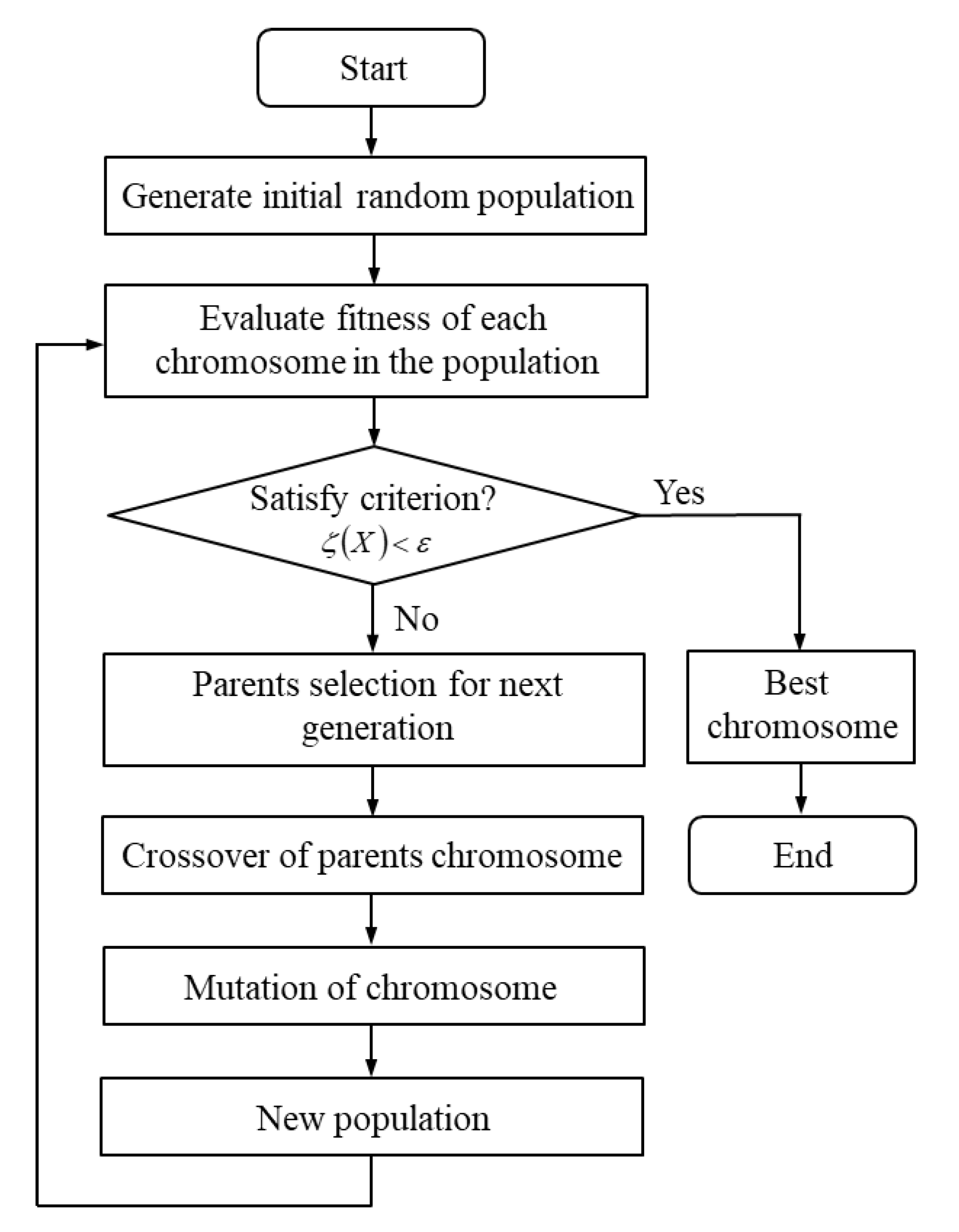
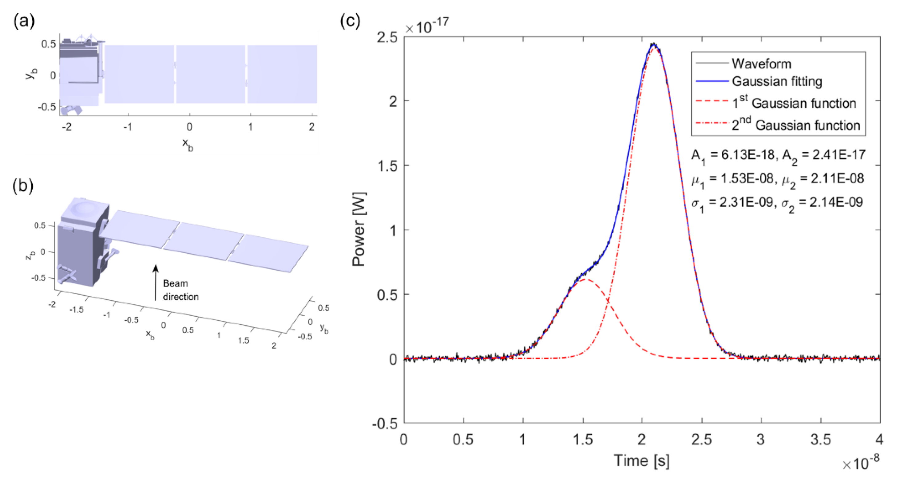
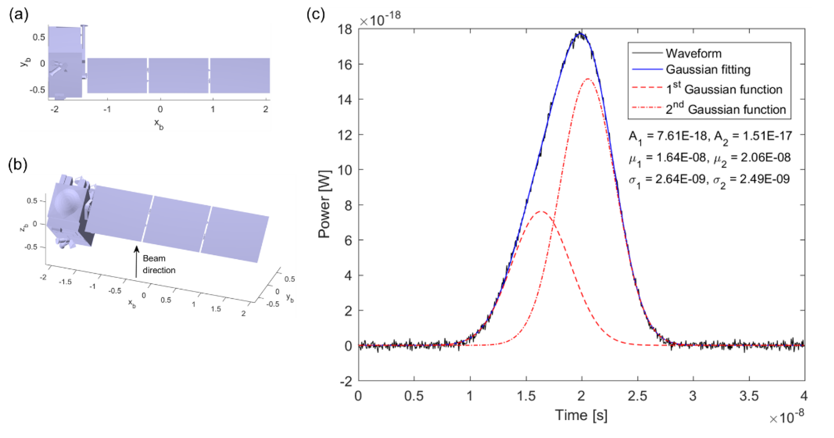
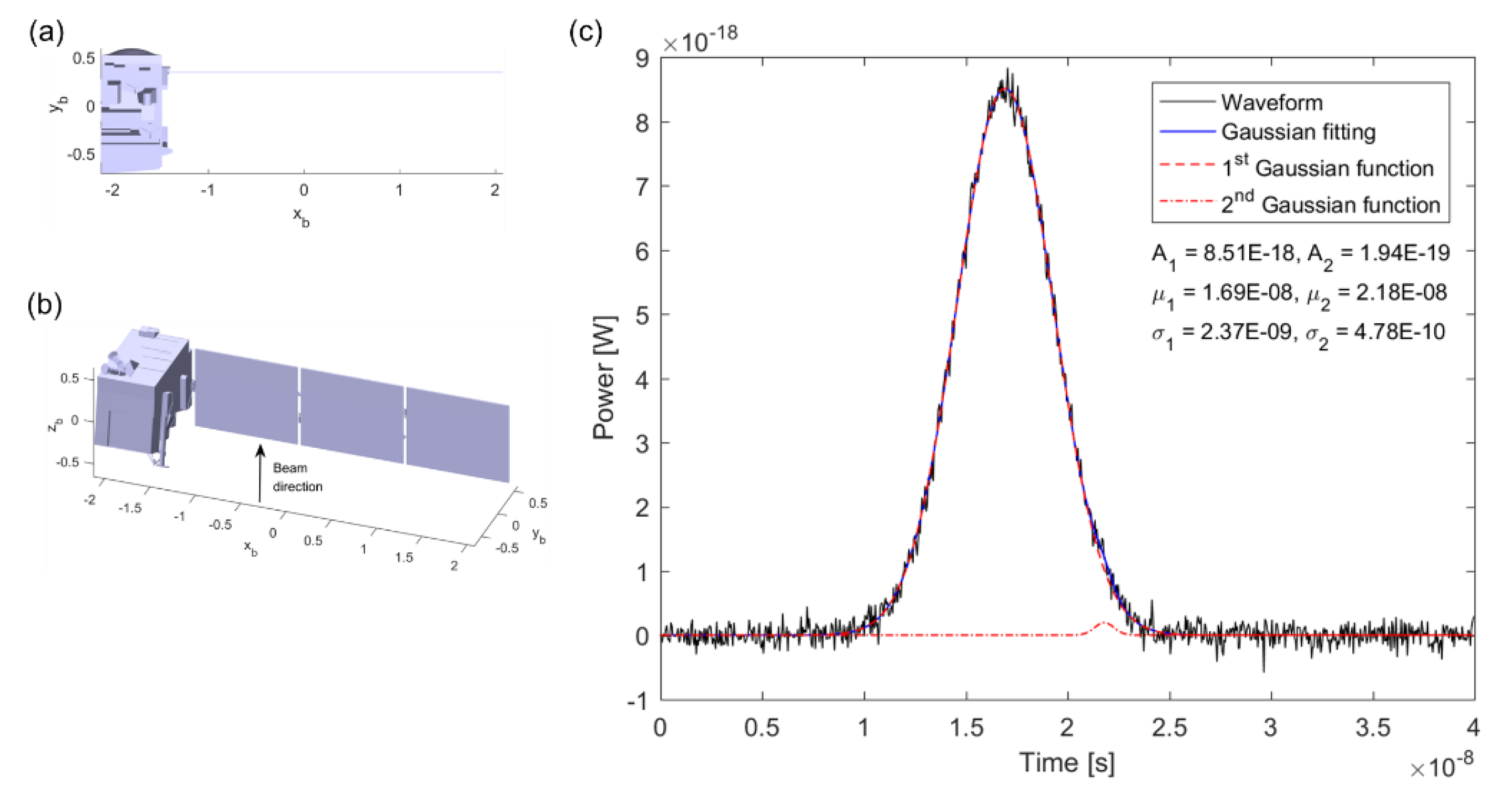
3. Genetic Algorithm for Gaussian Decomposition

The returned laser pulses are distorted by the cross-section characteristics (i.e., the scattering properties of targets) even though the transmitted pulses are Gaussian functions. However, it is assumed that the returned laser pulse from a small grid follows a Gaussian distribution in the time domain and then the ELPW summing the returned pulses is also represented by a series of Gaussian functions [29]. According to the analysis work of returned waveform [38], more than 98% of the observed waveforms with a topographic lidar could be correctly fitted with the sum of Gaussian functions. Therefore, the ELPW can be fitted with a mixture of Gaussian functions as follows [39]:

$$f\left(X,t\right)={\displaystyle \sum _{i=1}^n{A}_i\exp \left(-\frac{{\left(t-{\mu }_i\right)}^2}{2{\sigma }_i^2}\right)},$$

(23)

where $n$ is the number of Gaussian functions, and Gaussian parameters of $X_i=\left\{A_i,{\mu }_i,{\sigma }_i\right\}$ are the amplitude, position and half-width of the ith Gaussian function, respectively.

The Gaussian parameters are determined by the Gaussian decomposition so that Equation (23) fits the ELPW given by Equation (7) with a prescribed accuracy $\epsilon$ using some number of Gaussian functions:

$$\zeta \left(X\right)=\frac{1}{N_T}{{\displaystyle \sum _{k=1}^{N_T}\left[P_r\left(t_k\right)-f\left(t_k\right)\right]}}^2<\epsilon ,$$

(24)

where $t_k$ is the discrete time, and $N_T$ is the total number of discrete time intervals. There are several methods for the Gaussian decomposition, e.g., non-linear least square approach, maximum likelihood estimate, and stochastic approach [38]. The genetic algorithm (GA) is employed for the Gaussian decomposition in this study, which is a parameter optimization technique inspired by natural evolution using the concepts of mating, mutation, crossover, and selection [40,41].

The GA is briefly addressed in this section because it is only used as a tool to find Gaussian parameters. The GA works by building a population of chromosomes which is a set of potential solutions to Equation (24). The fitness $\zeta \left(X,t\right)$ of each chromosome in the population is evaluated and then a new population is created by repeating the following steps until the fitness of a new chromosome is satisfied: selection, crossover, and mutation. A probabilistic selection is performed based on the chromosome’s fitness such that the better chromosomes have an increased chance of being selected to reproduce into the next generation. The selected chromosomes, generally called parents, are to be mixed and recombined for the production of offspring in the next generation. In order to facilitate the GA evolution cycle, there are two fundamental operators: crossover and mutation. Based on the crossover and mutation probabilities, crossover takes two chromosomes and produces two new offsprings while mutation alters one chromosome to produce a single new offspring. A more complete explanation of the GAs can be found in the book by Davies [40]. The Gaussian decomposition based on the GA was implemented using the Matlab toolbox [42] and the flowchart of the GA process is shown in Figure 1.

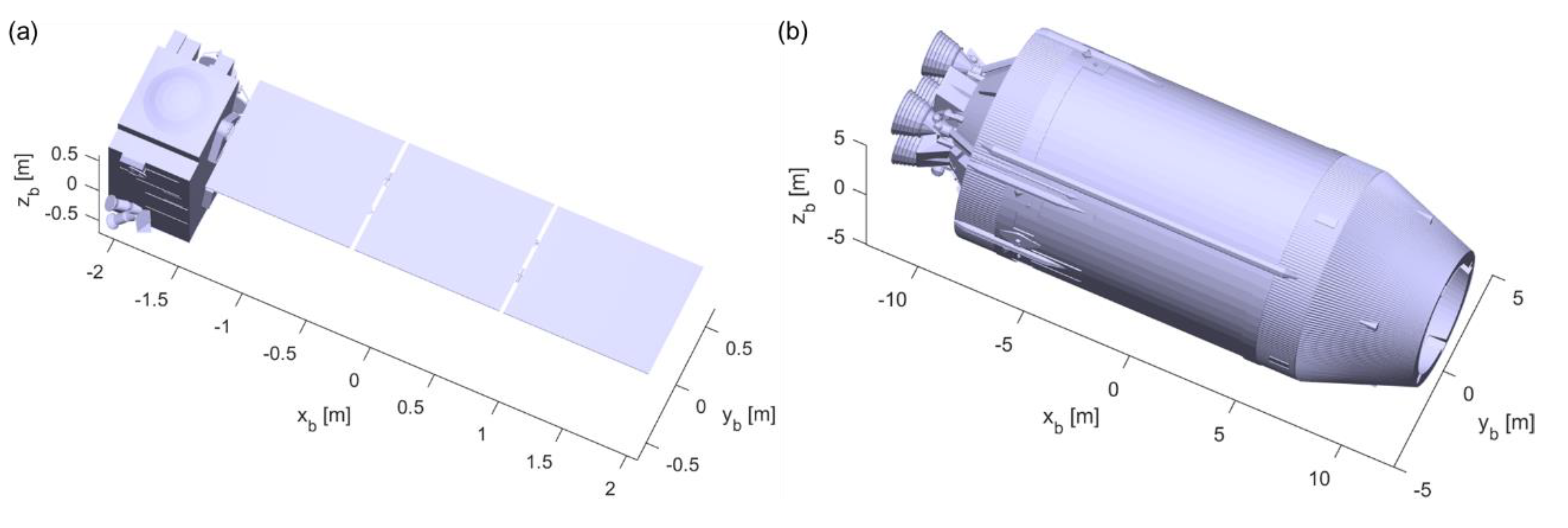
4. Simulation and Analysis of Laser Pulse Waveform

Two types of space debris were simulated to investigate the relationship between ELPW and orientation: defunct satellite (dimensions: 4.2 × 1.3 × 1.3 m) and rocket body (dimensions: 24.9 × 10.0 × 10.0 m). As shown in Figure 2, representing 3-dimensional models available from the NASA resources (https://nasa3d.arc.nasa.gov), the defunct satellite consists of a bus module, a solar panel, and small payloads, while the rocket body consists of five rocket engines, forward and aft skirts, tank and thrust structures, and an aft interstage. To generate the ELPW similar to the real measurement environment, the surface is made up of 113,241 grids for the defunct satellite, and 3,232,611 grids for the rocket body, respectively.

We performed a numerical simulation by considering the slant range $R_O$ of 500 km from the ground station to the origin of body frame, a zenith angle ${\theta }_z$ of 50 degrees, the ground station height $h_s$ of 1000 m, and the grid reflectivity $\rho$ of 0.175. Taking the clear sky (V = 15 km) and 1,064 nm wavelength of the laser beam into account, the atmospheric attenuation coefficient is $\sigma \left(\lambda ,V,0\right)=0.16$, and the cirrus cloud thickness $C_T$ of 0.5 km is considered.

The following parameters related to the NEP are also used for the numerical simulation: the electrical bandwidth $B=100\mathrm{MHz}$, the surface and bulk dark currents $I_{ds}=20\mathrm{nA}$ and $I_{db}=50\mathrm{nA}$, respectively, the detector gain $G=30$, the excess noise factor $F_A=0.25$, the detector quantum efficiency ${\eta }_Q=0.38$, the spectral radiance of the sky $I_{\lambda }=4.0\times {10}^{-8}\mathrm{watts}/{\mathrm{cm}}^2\cdot \mathrm{ster}\cdot \mu m$, the receiver field of view ${\Omega }_{FoV}=25\mathrm{arcsec}$, the bandwidth of the optical bandpass filter $\Delta {\lambda }_F=1\mathrm{nm}$, the amplifier temperature T = 19 °C, the noise factor $F_N=1.5$, and the load resistance $R_L=1,000\Omega$. In addition, the optical parameters related to the transmitter and receiver are summarized in

Table 1. Optical parameters of transmitter and receiver.

Parameter Description	Symbol	Value
Laser wavelength	$\lambda$	1064 nm
Transmitted power	$P_T$	60 W
Pulse energy (repetition rate)	-	60 J (1 Hz)
Full width at half maximum	FWHM	5 ns
Transmitting optical efficiency	${\eta }_T$	0.8
Divergence half angle	${\theta }_D$	10 arcsec
Telescope area	$A_R$	0.25π m2
Receiving optical efficiency	${\eta }_R$	0.7
Optical filter transmittance	${\eta }_F$	0.5

.

Considering that the laser beam is transmitted from the ground station at sea level to the space debris located at the slant range of 500 km, Figure 3 shows the beam spreading and broadening in terms of the atmospheric turbulence condition, zenith angle, and inner scale factor. The beam spreading due to the atmospheric turbulence has a considerable influence on the received power because the beam size can increase more than 2 times under the strong turbulence condition ($A_0=1.5\times {10}^{-13}{m}^{-2/3},\nu =30m/s$) and high zenith angle (${\theta }_Z=70\mathrm{deg}$). The beam broadening in time is little affected by the inner scale factor even though it suffers from the turbulence condition as well as the zenith angle. It is shown that the beam broadening effect decreases as the transmitting pulse width increases and that the effect also increases as the turbulence strength and zenith angle increase. In contrast to the nanosecond regime of the transmitted pulse width, the beam broadening is too significant in the femtosecond regime to be neglected for the ELPW analysis. However, the beam broadening is negligible in this study because the transmitted pulse width is in the order of nanoseconds. Regarding the beam spreading, the most commonly used values ($A_0=1.7\times {10}^{-14}{m}^{-2/3},\nu =21m/s$) are employed for the ELPW simulation.

Because of the small beam divergence, the DLR system controls the laser beam to the direction of a pre-determined position in space based on the predicted ephemeris. However, the target of space debris may deviate a little from the axis of beam propagation even though the receiver detects the echo signal from the target located within the coverage of beam divergence. The pointing error illustrated in Figure 4a can be reduced if an acquisition camera is employed to detect space debris illuminated by sunlight, which has an effect on the ELPW intensity as shown in Equation (1). Assuming that the space target is translated from the axis of beam propagation to the y-axis with pointing error $\varphi$, Equation (6) can be rewritten as

$$G_i\left(t\right)=\frac{2}{\pi W_{eff}^2\left(z\right)}\exp \left[-2\frac{x_{b,i}^2+{\left(R_O\sin \varphi +y_{b,i}\right)}^2}{W_{eff}^2\left(z\right)}\right]\cdot \frac{1}{\sqrt{2\pi }{\tau }_R}\exp \left[-\frac{1}{2{\tau }_R^2}{\left(t-\frac{2R_i}{c}\right)}^2\right],$$

(25)

where $\left(x_{b,i},y_{b,i}\right)$ is the coordinate of the ith grid on the body frame, and $R_O$ is the distance to the origin of the body frame. Figure 4b shows the ELPWs of defunct satellite in terms of the pointing error. Compared to the ELPWs for three pointing errors ($\varphi =0,3,5\mathrm{arcseconds}$), the ELPW intensity decreases with the same shapes as the pointing error increases. In addition, two pointing errors ($\varphi =5,-5\mathrm{arcseconds}$) cause some ELPW shape differences because the reflected surface of the defunct satellite is not symmetric with respect to the z-axis. But the difference of two shapes can be mitigated if a flattened Gaussian beam in which the energy distribution is nearly identical on the cross-section of the laser beam [43] is used. Thus the pointing error was not considered in the ELPW simulation.

The analytic expression related to the pulse broadening for laser altimeters [44] is introduced for the ELPW analysis:

$${\sigma }_R^2=\left({\sigma }_0^2+{\sigma }_h^2\right)+\frac{4\mathrm{Var}\left(\Delta \xi \right){\cos }^2{S}_{\left|\right|}}{c^2{\cos }^2\left(\phi +S_{\left|\right|}\right)}+\frac{4z^2{\tan }^2{\theta }_D}{c^2{\cos }^2\phi }\left[{\tan }^2{\theta }_D+{\tan }^2\left(\phi +S_{\left|\right|}\right)+\frac{{\tan }^2{S}_{\perp }{\cos }^2{S}_{\left|\right|}}{{\cos }^2\left(\phi +S_{\left|\right|}\right)}\right],$$

(26)

where ${\sigma }_h$ is the rms width of the receiver impulse response, $\Delta \xi$ is the surface roughness, and $\phi$ is the nadir angle of the laser beam. $S$ is the surface slope that consists of two components, namely a surface slope parallel to the nadir direction ($S_{\left|\right|}$) and a surface slope normal to nadir direction ($S_{\perp }$). According to Equation (26), the received pulse width is also broadened by the nadir angle and the target surface characteristics: surface roughness and slope of the ground target, and beam curvature. The nadir angle is negligible in this debris study because the reflected surface of the space debris is so small compared to the footprint of the laser altimeter that the reflected surface area is the same regardless of the nadir angle and thus makes no impact on the pulse broadening. In place of the nadir angle, the reflected surface area of space debris has an influence on the pulse broadening.

Figure 5, Figure 6, Figure 7 and Figure 8 show the echo waveforms as well as the Gaussian decomposition results for four orientations of the defunct satellite. The starting point of the range gate is determined to be arbitrary but the same for the simulations of four orientations (i.e., $t=0$ in the x-axis) in order to more easily compare and analyze the ELPWs. Unlike the Gaussian decomposition in Figure 8, the ELPWs in Figure 5, Figure 6 and Figure 7 were decomposed into two Gaussian functions because the reflected surface is characterized by two main elements: the bus module and the solar panel. The first Gaussian function is related to the bus module and the second one corresponds to the solar panel because the range to the bus module is shorter than that to the solar panel (i.e., ${\mu }_1<{\mu }_2$). The half-width of the first Gaussian function (${\sigma }_1$) in Figure 6 is larger than that in Figure 5 because the cross-section area of the reflected bus module is larger and consists of two surfaces of the bus module which cause larger roughness. The half-width of the second Gaussian function (${\sigma }_2$), corresponding to the solar panel in Figure 6, is also larger than that in Figure 5 even though the cross-section area of the reflected solar panel is smaller than that in Figure 5. The larger value of ${\sigma }_2$ results from the solar panel slope being normal to the beam direction (i.e., $S_{\perp }$) due to the 45° rotation about the x-axis. In the case of the defunct satellite orientation with -90° rotation about the x-axis as shown in Figure 7, the amplitude of the second Gaussian function is very small because the solar panel surface is perfectly parallel to the beam direction and thus the cross-section area is small. As shown in Figure 8, the second Gaussian function cannot fit the second curve in the ELPW well, which implies that the reflected surface is more complex than shown in Figure 5, Figure 6 and Figure 7 and the second curve is not separated into the bus module and solar panel elements.

Figure 9 shows two Gaussian decomposition results based on 3 and 4 Gaussian functions for the ELPW given in Figure 8, both of which fit the ELPW well. According to the orientation shown in Figure 8b, it is obvious that the first Gaussian function corresponds to the bus module and that the others result from the combination of the bus module and solar panel elements. The half-width of the Gaussian functions (${\sigma }_2$ and ${\sigma }_3$ in Figure 9a, ${\sigma }_2$ and ${\sigma }_4$ in Figure 9b) is larger than ${\sigma }_2$ of Figure 5 due to the solar panel slope parallel to the beam direction ($S_{\left|\right|}$), even though the cross-section area of the solar panel is smaller than that in Figure 5. The second curve in the ELPW was decomposed into 2 or 3 Gaussian functions, which can be also decomposed into many Gaussian functions by adding small Gaussian functions such as the third Gaussian function in Figure 9b. The complex reflected surface requires many Gaussian functions for the Gaussian decomposition and then makes the explicit analysis difficult in relation to the orientation of space debris.

The Gaussian decomposition results including the ELPWs are also shown in Figure 10, Figure 11, Figure 12 and Figure 13 for four kinds of orientations of the rocket body. Unlike the ELPWs of the defunct satellite, the size of the rocket body is so large that the noise power is very weak compared to the received power. In addition, the reflected surface is too complex compared to the defunct satellite to fit the ELPWs well even by using several Gaussian functions. Therefore, the total number of Gaussian functions ($n$) is selected as the smallest number that satisfies the criterion of Equation (24). As shown in Figure 10, the first two Gaussian functions corresponding to the first peak represent the forward and aft skirts as well as the tank structure because their shapes are cylindrical, and the other Gaussian functions correspond to five rocket engines, the thrust structure and the aft interstage. The ELPWs in Figure 11 and Figure 12 are so complex that each Gaussian function cannot be exactly in one-to-one correspondence with the components of the rocket body. Compared to the narrow distribution of ELPW in Figure 10, the wide distribution of ELPWs in Figure 11 and Figure 12 results from the rocket body slope parallel to the beam direction ($S_{\left|\right|}$). However, the ELPW has the distinctive shape subjected to the orientation of the rocket body, which enables orientation information to be achieved. Regarding the Gaussian decomposition in Figure 13, the first two Gaussian functions represent five rocket engines while the next three Gaussian functions correspond to the thrust structure and the sixth small Gaussian function comes from all five rocket engines.

It was shown that the orientation of a defunct satellite and a rocket body have a distinctive shape in the ELPW and the Gaussian functions that result from the Gaussian decomposition, which are a tool to characterize the orientation in more detail. The ELPW feature resulted from a single laser pulse that can provide sufficient information for the orientation determination of space debris. However, there is also a possibility in practical application that the ELPW features do not characterize the orientation of the space target due to its simple shape. If the ELPWs are available sequentially while the DLR is activated, the ELPW changes not only in shape but also in amplitude, which can provide more useful information for the orientation determination of space targets including even tumbling space debris. A number of small satellites, especially CubeSats which have simple and cubic shapes, have now been launched into space for scientific and commercial missions. It is difficult to determine the orientation of defunct CubeSats from the ELPW analysis even though a higher power laser is employed since the ELPW does not indicate the distinct features depending on their orientations because of a simple and cubic shape. But the orientation information of CubeSats is not relatively important in terms of the orbital prediction because the cross-sectional area variation is negligible over the entire orbit in computing the atmospheric drag and solar radiation pressure.

5. Conclusions

Orientation information of space debris is important to improve the orbital prediction accuracy for mitigation or elimination of a significant threat to not only human space activities but also operational satellites. The ELPW records the scattering signals from the space target surface and thus reflects the target shape in the direction of laser beam propagation. The new method based on the ELPW analysis was proposed to achieve the orientation information of space debris because it has no measurement constraints, unlike the photometry, AO and SLR technologies. This paper discussed the feasibility of using ELPW for the orientation determination of space debris by numerical simulations for a defunct satellite and a rocket body. By assuming that the reflected surface consists of small grids, the mathematical model was derived to generate the ELPW and also took into account the temporal beam broadening and spatial spreading due to the atmospheric turbulence. The beam broadening is so significant only in the femtosecond regime; it is negligible in the numerical simulation using the nanosecond pulse laser. Gaussian decomposition based on a genetic algorithm was employed to the ELPWs in order to analyze the orientation features. In particular, Gaussian functions obtained from the Gaussian decomposition were able to characterize the orientation features in more detail for a defunct satellite with a simpler configuration than a rocket body. It was demonstrated from the numerical simulations that the ELPW had a distinctive shape corresponding to the orientation of space debris, and therefore it could be considered as a feasible method to provide orientation information. Future works will focus on machine learning as a powerful tool to identify the orientation based on waveform shape recognition.

References

1. Vallado, D.A.; Finkleman, D. A critical assessment of satellite drag and atmospheric density modeling. Acta Astronautica 2014, 95, 141–165. [Google Scholar] [CrossRef]
2. Yanagisawa, T.; Kurosaki, H. Shape and motion estimate of LEO debris using light curves. Adv. Space Res. 2012, 50, 136–145. [Google Scholar] [CrossRef]
3. Santoni, F.; Cordelli, E.; Piergentili, F. Determination of disposed upper-stage attitude motion by ground-based optical observations. J. Spacecraft Rock. 2013, 50, 701–708. [Google Scholar] [CrossRef]
4. Kanzler, R.; Silha, J.; Schildknecht, T.; Fritsche, B.; Lips, T.; Krag, H. Space debris attitude simulation-iOTA (In-Orbit Tumbling Analysis). In Proceedings of the 15th Advanced Maui Optical and Space Surveillance Technologies (AMOS) Conference, Maui, HI, USA, 15–18 September 2015. [Google Scholar]
5. Koshkin, N.; Korobeynikova, E.; Shakun, L.; Strakhova, S.; Tang, Z.H. Remote sensing of the EnviSat and Cbers-2B satellites rotation around the centre of mass by photometry. Adv. Space Res. 2016, 58, 358–371. [Google Scholar] [CrossRef]
6. Koshkin, N.; Shakun, L.; Burlak, N. Ajisai spin-axis precession and rotation-period variations from photometric observations. Adv. Space Res. 2017, 60, 1389–1399. [Google Scholar] [CrossRef]
7. Silha, J.; Pittet, J.-N.; Hamara, M.; Schildknecht, T. Apparent rotation properties of space debris extracted from photometric measurements. Adv. Space Res. 2018, 61, 844–861. [Google Scholar] [CrossRef]
8. Bennet, F.; D’Orgeville, C.; Price, I.; Rigaut, F.; Ritchie, I.; Smith, C. Adaptive optics for satellite imaging and space debris ranging. In Proceedings of the 15th Annual Advanced Maui Optical and Space Surveillance Technologies (AMOS) Conference, Maui, HI, USA, 15–18 September 2015. [Google Scholar]
9. Copeland, M.; Bennet, F.; Zovaro, A.; Riguat, F.; Piatrou, P.; Korkiakoski, V.; Smith, C. Adaptive Optics for Satellite and Debris Imaging in LEO and GEO. In Proceedings of the 17th Annual Advanced Maui Optical and Space Surveillance Technologies (AMOS), Maui, HI, USA, 19–22 September 2017. [Google Scholar]
10. Copeland, M.; Bennet, F.; Rigaut, F.; Korkiakoski, V.; d’Orgeville, C.; Smith, C. Adaptive optics corrected imaging for satellite and debris characterization. In Proceedings of the SPIE 10703, Adaptive Optics Systems VI, Austin, TX, USA, 11 July 2018; p. 1070333. [Google Scholar]
11. Kucharski, D.; Otsubo, T.; Kirchner, G.; Koidl, F. Spin axis orientation of Ajisai determined from Graz 2 kHz SLR data. Adv. Space Res. 2010, 46, 251–256. [Google Scholar] [CrossRef]
12. Kucharski, D.; Kirchner, G.; Koidl, F. Spin parameters of nanosatellite BLITS determined from Graz 2 kHz SLR data. Adv. Space Res. 2011, 48, 343–348. [Google Scholar] [CrossRef]
13. Kucharski, D.; Otsubo, T.; Kirchner, G.; Bianco, G. Spin rate and spin axis orientation of LARES spectrally determined from satellite laser ranging data. Adv. Space Res. 2012, 50, 1473–1477. [Google Scholar] [CrossRef]
14. Kucharski, D.; Lim, H.-C.; Kirchner, G.; Hwang, J.-Y. Spin parameters of LAGEOS-1 and LAGEOS-2 spectrally determined from Satellite Laser Ranging data. Adv. Space Res. 2013, 52, 1332–1338. [Google Scholar] [CrossRef]
15. Kucharski, D.; Kirchner, G.; Koidl, F.; Fan, C.; Carman, R.; Moore, C.; Dmytrotsa, A.; Ploner, M.; Bianco, G.; Medvedskij, M. Attitude and spin period of space debris envisat measured by satellite laser ranging. IEEE Trans. Geosci. Rem. Sens. 2014, 52, 7651–7657. [Google Scholar] [CrossRef]
16. Kirchner, G.; Steindorfer, M.; Wang, P.; Koidl, F.; Kucharski, D.; Silha, J.; Schildknecht, T.; Krag, H.; Flohrer, T. Determination of attitude and attitude motion of space debris, using laser ranging and single-photon light curve data. In Proceedings of the 7th European Conference on Space Debris, Darmstadt, Germany, 18–21 April 2017. [Google Scholar]
17. Kucharski, D.; Kirchner, G.; Bennett, J.; Lachut, M.; Sos’nica, K.; Koshkin, N.; Shakun, L.; Koidl, F.; Steindorfer, M.; Wang, P. Photon pressure force on space debris TOPEX/Poseidon measured by Satellite Laser Ranging. Earth Space Sci. 2017, 4, 661–668. [Google Scholar] [CrossRef]
18. Schildknecht, T.; Linder, E.; Silha, J.; Hager, M.; Koshkin, N.; Korobeinikova, E.; Melikiants, S.; Shakun, L.; Strakhov, S. Photometric monitoring of non-resolved space debris and databases of optical light curves. In Proceedings of the 15th Advanced Maui Optical and Space Surveillance Technologies (AMOS) Conference, Maui, HI, USA, 15–18 September 2015. [Google Scholar]
19. Schildknecht, T.; Silha, J.; Pittet, J.-N.; Rachman, A. Attitude states of space debris determined from optical light curve observations. In Proceedings of the 1st IAA Conference on Space Situational Awareness (ICSSA), Orlando, FL, USA, 13–15 November 2017. [Google Scholar]
20. Zhao, S.; Steindorfer, M.; Kirchner, G.; Zheng, Y.; Koidl, F.; Wang, P.; Shang, W.; Zhang, Z.; Li, T. Attitude analysis of space debris using SLR and light curve data measured with single-photon detector. Adv. Space Res. 2020, 65, 1518–1527. [Google Scholar] [CrossRef]
21. Zhang, Z.-P.; Yang, F.-M.; Zhang, H.-F.; Wu, Z.-B.; Chen, J.-P.; Li, P.; Meng, W.-D. The use of laser range to measure space debris. Res. Astron. Astrophys. 2012, 12, 212–218. [Google Scholar] [CrossRef] [Green Version]
22. Sang., J.; Smith, C. Performance Assessment of the EOS Space Debris Tracking System. In Proceedings of the AIAA 2012-5018, AIAA/AAS Astrodynamics Specialist Conference, Minneapolis, MN, USA, 3–16 August 2012. [Google Scholar]
23. Kirchner, G.; Koidl, F.; Friederich, F.; Buske, I.; Volker, U.; Riede, W. Laser measurements to space debris from Graz SLR station. Adv. Space Res. 2013, 51, 21–24. [Google Scholar] [CrossRef]
24. Lim, H.-C.; Park, J.-U.; Kim, D.-J.; Seong, K.; Ka, N.-H. Laser Tracking Analysis of Space Debris using SOLT System at Mt. Gamak. J. Korean Soc. Aeronaut. Space Sci. 2015, 43, 830–837. [Google Scholar]
25. Li, Y.; Wu, Z. Targets recognition using subnanosecond pulse laser range profiles. Opt. Express 2010, 18, 16788–16796. [Google Scholar] [CrossRef]
26. Johnson, S.E. Effect of target surface orientation on the range precision of laser detection and ranging systems. J. Appl. Remote Sens. 2009, 3, 033564. [Google Scholar] [CrossRef]
27. Richmond, R.D.; Cain, S.C. Direct-Detection LADAR Systems; SPIE: Washington, DC, USA, 2010. [Google Scholar]
28. Abshire, J.B.; Sun, X.; Afzal, R.S. Mars orbiter laser altimeter: Receiver model and performance analysis. Appl. Opt. 2000, 39, 2449–2460. [Google Scholar] [CrossRef] [Green Version]
29. Wagner, W.; Ullrich, A.; Ducic, V.; Melzer, T.; Studnicka, N. Gaussian decomposition and calibration of a novel small-footprint full-waveform digitizing airborne laser scanner. ISPRS J. Photogramm. Remote Sens. 2006, 60, 100–112. [Google Scholar] [CrossRef]
30. Hao, Q.; Cheng, Y.; Cao, J.; Zhang, F.; Zhang, X.; Yu, H. Analytical and numerical approaches to study echo laser pulse profile affected by target and atmospheric turbulence. Opt. Express 2016, 24, 25026–25042. [Google Scholar] [CrossRef] [PubMed] [Green Version]
31. Degnan, J.J. Milimeter Accuracy Satellite Laser Ranging: A Review. Geodyn. Ser. 1993, 25, 133–162. [Google Scholar]
32. Gao, M.; Li, Y.; Gong, L.; Lv, H. Pulse broadening and beam spread of polarized laser pulse beam on slant path in turbulence atmospheric. Optik 2015, 126, 4651–4657. [Google Scholar] [CrossRef]
33. Andrews, L.C.; Phillips, R.L. Laser Beam Propagation through Random Media; SPIE Optical Engineering Press: Bellingham, WA, USA, 1998. [Google Scholar]
34. Kaushal, H.; Kaddoum, G. Optical Communication in Space: Challenges and Mitigation Techniques. IEEE Commun. Surv. Tutor. 2016, 19, 57–96. [Google Scholar] [CrossRef] [Green Version]
35. Young, C.Y.; Andrews, L.C.; Ishimaru, A. Time-of-arrival fluctuations of a space-time Gaussian pulse in weak optical turbulence: An analytic solution. Appl. Opt. 1998, 37, 7655–7660. [Google Scholar] [CrossRef]
36. Der, S.; Redman, B.; Chellappa, R. Simulation of error in optical radar range measurements. Appl. Opt. 1997, 36, 6869–6874. [Google Scholar] [CrossRef] [PubMed]
37. Hemmati, H. Deep Space Optical Communications; Jet Propulsion Laboratory, California Institute of Technology: Pasadena, CA, USA, 2006.
38. Mallet, C.; Bretar, F. Full-waveform topographic LiDAR: State-of-the-art. ISPRS J. Photogramm. Remote Sens. 2009, 64, 1–16. [Google Scholar] [CrossRef]
39. Zhou, T.; Popescu, S. waveformlidar: An R Package for Waveform LiDAR Processing and Analysis. Remote Sens. 2019, 11, 2552. [Google Scholar] [CrossRef] [Green Version]
40. Davies, L. Handbook of Genetic Algorithms; Van Nostrand Reinhold: New York, NY, USA, 1991. [Google Scholar]
41. Man, K.F.; Tang, K.S.; Kwong, S. Genetic algorithms: Concepts and applications. IEEE Trans. Ind. Electron. 1996, 43, 519–534. [Google Scholar] [CrossRef]
42. Houck, C.; Joines, J.; Kay, M. A Genetic Algorithm for Function Optimization: A Matlab Implementation, NCSU-IE Technical Report 95-09; North Carolina State University: Raleigh, NC, USA, 1996. [Google Scholar]
43. Gori, F. Flattened gaussian beam. Opt. Commun. 1994, 107, 335–341. [Google Scholar] [CrossRef]
44. Gardner, C.S. Ranging performance of satellite laser altimeters. IEEE Trans. Geosci. Remote Sens. 1992, 30, 1061–1072. [Google Scholar] [CrossRef] [Green Version]
Figure 1. Flowchart of the genetic algorithm.
Remotesensing 12 01659 g001
Figure 2. 3-dimentionl images of (a) defunct satellite, and (b) rocket body.
Remotesensing 12 01659 g002
Figure 3. (a) Beam spreading and (b) broadening, due to the atmospheric turbulence.
Remotesensing 12 01659 g003
Figure 4. Illustration of (a) laser tracking with a pointing error, and (b) the echo laser pulse waveforms (ELPWs) for four pointing errors. The ELPWs were obtained by employing the reflected surface or orientation identical to Figure 5.
Remotesensing 12 01659 g004
Figure 5. The (a) reflected surface, (b) orientation of defunct satellite, and (c) the echo waveform and 2 Gaussian functions obtained from the Gaussian decomposition, for no rotation w.r.t. Figure 2a.
Remotesensing 12 01659 g005
Figure 6. The (a) reflected surface, (b) orientation of defunct satellite, and (c) the echo waveform and 2 Gaussian functions obtained from the Gaussian decomposition for 45° rotation about the x-axis w.r.t. Figure 2a.
Remotesensing 12 01659 g006
Figure 7. The (a) reflected surface, (b) orientation of defunct satellite, and (c) the echo waveform and 2 Gaussian functions obtained from the Gaussian decomposition for −90° rotation about the x-axis w.r.t. Figure 2a.
Remotesensing 12 01659 g007
Figure 8. The (a) reflected surface, (b) orientation of defunct satellite, and (c) the echo waveform and 2 Gaussian functions obtained from the Gaussian decomposition for −45° rotation about the y-axis w.r.t. Figure 2a.
Remotesensing 12 01659 g008
Figure 9. Gaussian decomposition results using (a) 3 Gaussian functions and (b) 4 Gaussian functions for the ELPW in Figure 8c.
Remotesensing 12 01659 g009
Figure 10. The (a) reflected surface, (b) orientation of rocket body, and (c) the echo waveform and 5 Gaussian functions obtained from the Gaussian decomposition for no rotation w.r.t. Figure 2b.
Remotesensing 12 01659 g010
Figure 11. The (a) reflected surface, (b) orientation of rocket body, and (c) the echo waveform and 7 Gaussian functions obtained from the Gaussian decomposition for −45° rotation about the y-axis w.r.t. Figure 2b.
Remotesensing 12 01659 g011
Figure 12. The (a) reflected surface, (b) orientation of rocket body, and (c) the echo waveform and 7 Gaussian functions obtained from the Gaussian decomposition for 45° rotation about the y-axis w.r.t. Figure 2b.
Remotesensing 12 01659 g012
Figure 13. The (a) reflected surface, (b) orientation of rocket body, and (c) the echo waveform and 7 Gaussian functions obtained from the Gaussian decomposition for −90° rotation about the y-axis w.r.t. Figure 2b.
Remotesensing 12 01659 g013