Calibration of an Airborne Interferometric Radar Altimeter over the Qingdao Coast Sea, China

Abstract

Calibration/Validation (Cal/Val) of satellite altimeters is fundamental for monitoring onboard sensor performance and ensuring long-term data quality. As altimeter technology has been evolving rapidly from profile to wide swath and interferometric altimetry, different requirements regarding Cal/Val have emerged. Most current Cal/Val technology has been developed for conventional profile altimeters, whereby satellite observations are compared against measurements at one point along orbit lines. However, the application of this type of Cal/Val technique to swath interferometric altimeters with two-dimensional measurements is difficult. Here, we propose a new strategy for the evaluation of interferometric altimeters based on comparison of wave-induced sea surface elevation (WSSE) spectra from one- and two-dimensional measurements. This method assumes that the WSSE variance of an equilibrium wave field is uniform and can be measured equivalently in the space or time domains. The method was first tested with simulated data and then used to evaluate the performance of an airborne interferometric radar altimeter system (AIRAS) using Global Navigation Satellite System (GNSS) buoy measurements. The differences between the WSSE variances from the AIRAS and two GNSS buoys were below 8 cm², corresponding to a standard deviation of 2.8 cm, which could serve as a reference for the WSSE error over the scale range of waves. The correlation coefficient between the AIRAS and GNSS buoys was approximately 0.90, indicating that the error was small relative to the WSSE signals. In addition, the sea surface height (SSH) difference measured by the AIRAS was compared with that derived from the GNSS buoys at two sites. The results indicated that the error of the SSH difference was 3 cm. This approach represents a possible technique for the Cal/Val of future spaceborne/airborne interferometric altimeters; however, additional experiments and applications are needed to verify the feasibility of this method.

1. Introduction

Monitoring of altimetry products through calibration and validation (Cal/Val) is essential for detecting any biases and trends in satellite observations and thus for ensuring long-term consistency and continuity of measurements obtained from different missions [1]. There are four principal long-running Cal/Val sites around the world: (1) the Harvest platform site operated by the Jet Propulsion Lab/NASA (USA) [2,3,4,5], (2) the Corsica site run by the French Space Agency (CNES) [6,7,8,9,10], (3) the Crete/Gavdos site managed by the Technical University of Crete (Greece) and the European Space Agency [11,12,13], and (4) the Bass Strait site in Australia run by the University of Tasmania [14,15,16]. In China, the Qianli Yan site in the Yellow Sea off the coast of Qingdao has also been operated in support of the Chinese HY-2 satellite altimeter as well as the Jason, Envisat, and Sentinel-3 series of satellites [17,18,19]. In addition, Cal/Val sites such as the one on Lake Issykul, Kyrgyzstan, where certain oceanic error sources are reduced, are also used to provide altimeter biases [20,21,22,23]. The main Cal/Val methods applied at the above sites are based on comparison of altimetry-derived sea surface height (SSH) with ground-based measurements determined using in situ tide gauges, precise positioning, and/or Global Navigation Satellite System (GNSS) buoys [24]. These techniques have worked well in along-track calibration of conventional nadir altimeters for more than 25 years [5].

Since the 1970s, satellite altimetry technology has improved gradually in terms of both spatiotemporal resolution and accuracy. Resolution can be roughly classified into three evolution phases: the “diamond” (1970–1980s), “grid” (1990–2010), and “pixel” (2020s onward) resolution phases [25]. In 2021, a new type of altimeter is scheduled for launch (e.g., in the surface water and ocean topography (SWOT) mission) that will be able to realize “pixel” resolution over wide swaths of approximately 120 km [26,27,28]. Similarly, China’s new “Guanlan” science mission, designed with a dual-frequency (Ku-band and Ka-band) interferometric altimeter and an ocean lidar sensor, will advance oceanic remote sensing [25]. Until now, existing Cal/Val technologies have all been designed to serve profile altimeters that measure the sea surface only at nadir points. However, conventional calibration methods with Cal/Val sites at a single fixed point cannot fully satisfy the needs for calibrating wide-swath interferometric altimeters. Consequently, calibration of SWOT-like missions requires new Cal/Val methods.

For the SWOT mission, an additional profile altimeter will provide effective Cal/Val of the Ka-band radar interferometer at wavelengths longer than 120 km [26,29,30]. At wavelengths shorter than 120 km, an airborne radar interferometer (AirSWOT) using the same SWOT technology of wide-swath interferometry has been developed to measure the two-dimensional high-resolution SSH over the swath covered by the satellite [31,32]. However, proper operation of the AirSWOT still requires the support of in situ Cal/Val facilities such as GNSS buoys, gliders, and moorings [26]. In addition to the AirSWOT, a novel observing system simulation experiment was performed for the calibration of SSH determined by a wide-swath interferometric altimeter [33]. The SSH wavenumber spectrum was compared using simulated arrays of at least 20 station-keeping gliders or moorings under the wide-swath coverage. Then, the observing system simulation experiment was gradually improved by adding a multiscale data assimilation system [34]. However, it should be noted that such operations would encounter practical difficulties when performed in the real ocean.

The Cal/Val activity for the Chinese Guanlan science mission also represents a challenging and demanding task. Comprehensive in situ Cal/Val arrays, including GNSS buoys, gliders, moorings, pressure-inverted echo sounders, and coastal tide gauges, will be integrated to fulfil the Cal/Val requirements of the Guanlan mission for simultaneous high-resolution SSH retrievals over 166-km-wide swaths [25]. In addition to the Guanlan mission, an experimental interferometric altimeter sensor has already been deployed onboard the Tiangong-2 Space Laboratory, which collected high-resolution (40 m) SSH data in a swath approximately 20–40 km wide during 2016–2019 [35]. However, reports on the Cal/Val of the Tiangong-2 interferometric altimeter are rare.

In this paper, we report on a Cal/Val experiment of an airborne interferometric radar altimeter system (AIRAS) designed as an engineering test prototype for the future Guanlan science mission. This experiment used in situ SSH data collected by GNSS buoys and other sources such as tide gauges, wave buoys, and weather stations that were provided by a national oceanic observation station in Qingdao. The advantage of GNSS buoy data over station data is that buoys can be deployed in target areas along the track of the airborne or satellite platforms, which is vital for the Cal/Val of high-resolution interferometric altimetry data. Previous studies have illustrated the possibility of using wavenumber comparisons in the space domain using by a network of station-keeping glider data to achieve such altimetry calibration [33]. However, there is still a critical question of how to calibrate the interferometric altimeter measurements in the space domain by GNSS or other buoy measurements which are in the time domain. To tackle this problem, we divided the Cal/Val of the AIRAS into two parts: the relative SSH difference between the two GNSS buoy locations and the wave-induced sea surface elevation (WSSE) directly above the GNSS buoy locations. For the WSSE, we deduced a mathematical transform that could unify the power spectral density from space and time domains, which makes this comparison and calibration possible. To illustrate the feasibility of the proposed method, a simulation of wind-generated sea surface elevation was tested using the Pierson–Moskowitz wave spectrum [36]. For the relative SSH signal between the different locations of GNSS buoys, which is related primarily to the SSH difference caused by the geoid slope, we used a low-pass filter to remove part of the ocean wave signal in the GNSS buoy and AIRAS measurements. Then, the SSH difference observed by the AIRAS could be assessed using data from the GNSS buoys at two different locations.

Our research provides a solution to the problem of Cal/Val of airborne interferometric altimeters, which is a prerequisite step in the calibration of spaceborne interferometric altimeters [26]. We also proved that the AIRAS could measure small-scale wind-induced gravity waves with high accuracy, in addition to the determination of relative SSH variation. This work was undertaken within the scope of the Cal/Val activities for the future Guanlan science mission.

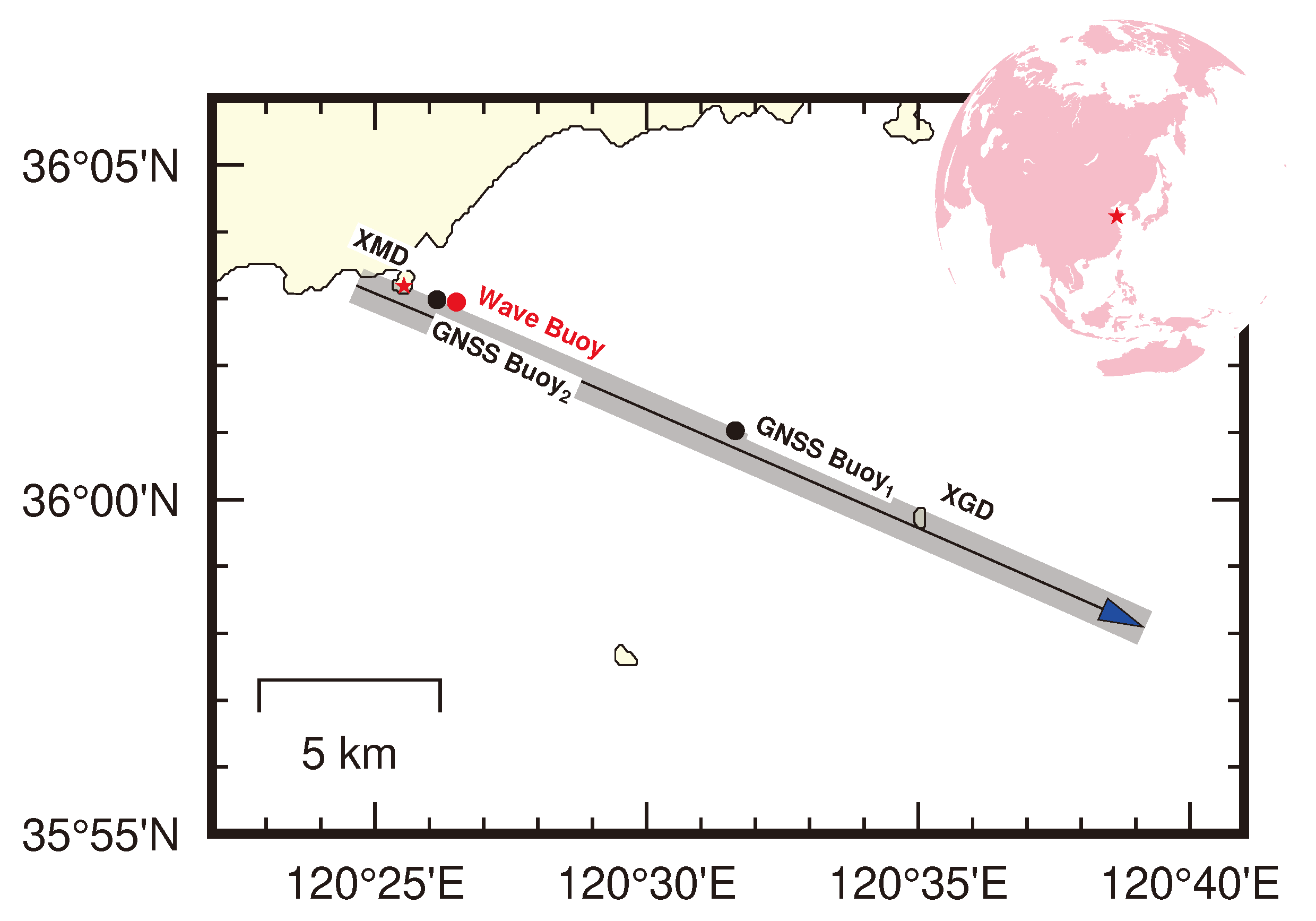
2. Basic Description of the Validation Campaign

The main purpose of the airborne experiment was to verify the concept of interferometry. The flight height of the aircraft was set to 3000 m to maintain both a low noise level and a high signal-to-noise ratio. Therefore, the swath width was approximately only 1 km (determined by the flight height). Because the positioning accuracy of the aircraft and that of the GNSS buoys decreased with distance from the GNSS reference stations on land, the aircraft was flown at a maximum distance of 20 km from the coast and the in situ Cal/Val GNSS buoys were deployed within approximately 10 km. The water depth being only 25 m in this shallow sea, the SSH signals seen at this scale mainly reflect sea surface changes caused by ocean waves and wind setup effects (the submesoscale signals are relatively small). We chose to conduct Cal/Val by studying the wave field.

Figure 1 shows the area of the Yellow Sea off the coast of Qingdao chosen for the field test, and the location of a nearby national oceanic observation station (XiaoMaiDao, XMD). This site was considered ideal for assessment of the AIRAS capacity to detect ocean dynamic signals of WSSE because it is a well-studied sea area populated with many oceanographic sensors operated by various institutes and national stations. It is also ideal for assessment of the capacity of the AIRAS to observe the SSH difference between different locations because the slope of the mean sea surface (MSS) within the area is approximately 3 cm/km (Figure 2).

The airborne campaign took place on March 31, 2019. It was coordinated by both the Qingdao National Laboratory for Marine Science and Technology and the Ocean University of China. The Beijing Institute of Radio Measurement designed the AIRAS hardware and modified one YUN-5 aircraft to carry the AIRAS instrument together with the airborne GNSS and inertial navigation system. The flight path of the aircraft is shown by the black line in Figure 1. As can be seen, the plan was for the aircraft to pass over stations XMD and XGD (XiaoGongDao) and to fly up to 20 km away from the coastline. Two GNSS reference stations were deployed at stations XMD and XGD to aid processing of the GNSS buoy and airborne GNSS data. The AIRAS aircraft position was determined using an airborne GNSS receiver operating at a sampling rate of 1 Hz, together with its inertial navigation system operating at 200 Hz. The AIRAS SSH data were collected over the XMD area, both on land and sea, at a flight height of 3000 m. Over the ocean, the SSH observations were collected with 0.3-m resolution, depending on flight height. The swath coverage (approximately 1-km width) of this airborne campaign is illustrated by the gray shading in Figure 1.

Two GNSS buoys, separated by a distance of 9 km, were deployed in the sea area of the AIRAS observation, which provided 1-Hz SSH data. After completion of the AIRAS campaign, GNSS buoy 1 was moved by ship to the location of buoy 2 to conduct cross validation of the buoys. In addition, tide gauge, wave buoy, and weather station data were also collected during this campaign. All these data helped with evaluation of the sea state conditions and provided suitable filters for the GNSS buoy measurements.

3. The AIRAS and in Situ Data

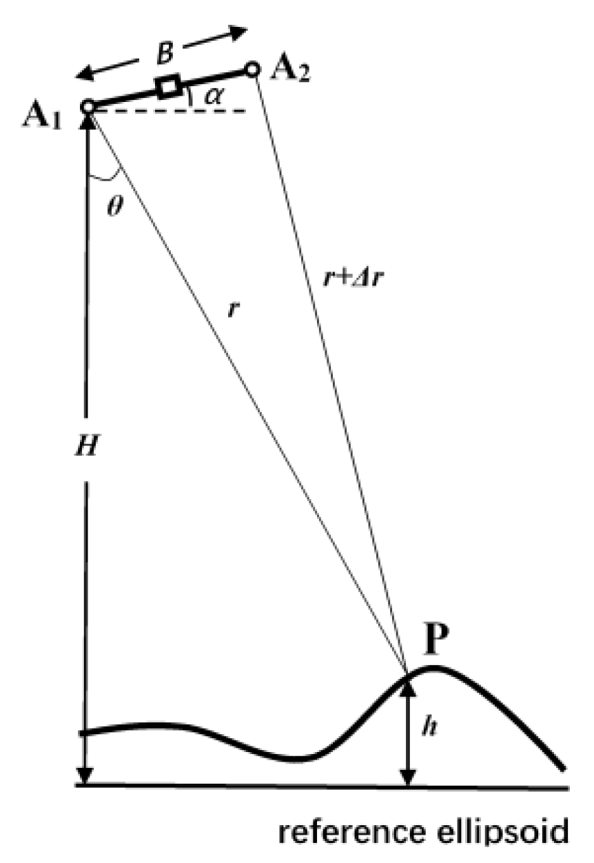
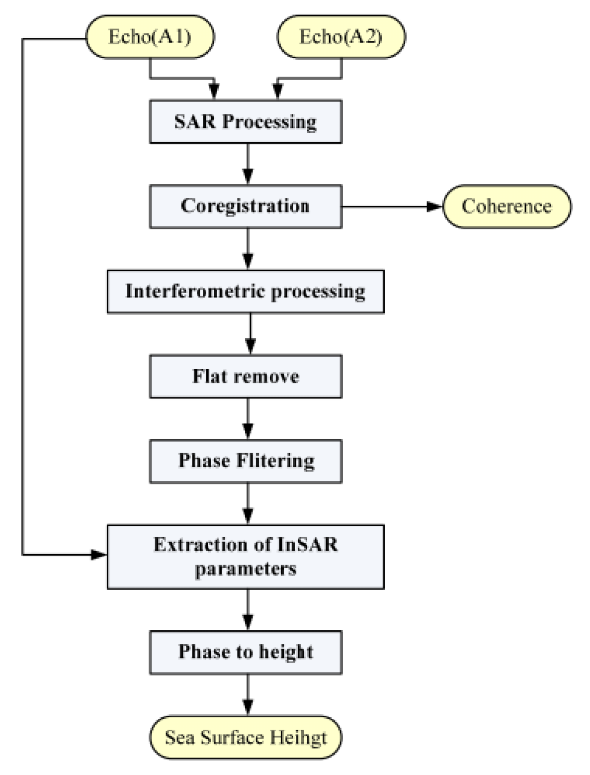
3.1. The Principle of AIRAS Measurements

Based on the interferometric synthetic aperture radar (InSAR) technique, we designed an imaging altimeter that could observe swaths of sea surface height extending from one to hundreds of kilometers with a small incidence angle (usually within 10${}^{\circ }$) near nadir. The AIRAS is designed for high-accuracy elevation mapping and this study marked the first time it was used to map two-dimensional SSH.

The principle of such a measurement technique, similar to InSAR sensors, is shown in Figure 3, where $A_1$ is the main antenna, $A_2$ is the auxiliary antenna, B is the baseline length, and $\alpha$ is the baseline roll angle. The orbital altitude above the reference ellipsoid of $A_1$ is H and the angle of incidence relative to target point P on the sea surface is $\theta$. Here, ${\Delta }r$ is the range difference between the two antenna returns. The height of target point P relative to the reference ellipsoid is h. From the geometric relations illustrated in Figure 3, the ellipsoidal height h of the sea surface at point P can be derived as follows [37]:

$$h=H-r\times cos\left\{\alpha +arcsin[\frac{B^2-{\left(\frac{\lambda \phi }{2\pi }\right)}^2-\frac{r\lambda \phi }{\pi }}{2rB}]\right\},$$

(1)

where $\phi$ represents the interferometric phase, and $\lambda$ is the return echo wavelength. Equation (1) establishes the relationship between elevation, slant range, and interferometric phase. By processing the echo signal, the slant range r and interferometric phase $\phi$ of the target relative to the main antenna can be obtained. Then, together with the antenna position parameters ($H,\alpha$ and $B)$, the elevation h of the sea surface can be determined.

The main interferometric altimeter parameters of the AIRAS are provided in

Table 1. The main parameters of the AIRAS in this campaign.

Parameter	Ka Band Interferometric Altimeter
Center frequency	35 GHz
Processed incidence angle	1–15${}^{\circ }$
Bandwidth	500 MHz
Pulse repetition frequency	2000 Hz
Range resolution	0.3 m
Azimuth resolution	0.3 m
Flight altitude	3000 m
Baseline length	30 cm

. Based on simulations, the expected precision of SSH derived by the AIRAS was 2.3 cm at a small angle of incidence (1${}^{\circ }$) and 5.0 cm at a large angle of incidence (15${}^{\circ }$). The average uncertainty in the determination of SSH over the entire observation region was expected to be 3.4 cm.

3.2. The AIRAS Sea Surface Height Determination

After the reflected signals from the sea surface were collected by the AIRAS interferometric altimeter sensor, SSHs were determined by following the data processing procedure shown in Figure 4. This procedure mainly involves processing of the synthetic aperture radar (SAR) and interferometric data measured by the two Ka-band radar antennas of the AIRAS. Finally, the SSHs were converted from the phase measurements. The reference surface adopted for the SSH data was the WGS-84 ellipsoid established through the onboard GNSS coordinates.

The original sea surface elevation measured by the AIRAS over the GNSS buoy locations is shown in the right-hand panels of Figure 5. The power spectrum (not shown here) indicated that signals with wavelengths of less than 3 m were mainly noise. Therefore, in the Cal/Val procedure, we employed a low-pass filter with a cut-off wavelength of 3 m to remove such noise. In addition, the AIRAS SSH includes relatively long wavelength signals that might be related to geoid signals [7]. Therefore, we used a high-pass filter with a cut-off wavelength of 150 m to remove the relatively long wavelength signals in the SSH spectrum [38]. After data filtering, the retained power spectrum preserved in the AIRAS data at wavelengths of 3–150 m mainly contained the WSSE. The band-pass filtered results are shown in the left-hand panels of Figure 5. This final airborne product was used in the Cal/Val procedure with the GNSS buoy data.

3.3. In Situ Data

As shown in Figure 1, the location selected for the AIRAS experiment was in the coastal sea offshore from XMD, Qingdao, China. Station XMD is part of the network of national oceanic observation stations in China, which has been monitoring SSH for more than 50 years. For our experiment, the data collected at station XMD, which included tide gauge, GNSS, weather station, and ocean wave buoy data, were used as important in situ data for calibration of the AIRAS. For that purpose, the tide gauge benchmark was connected to the GNSS permanent station through spirit levelling (Figure 6). Thus, the SSH reference of the tide gauges was the same as that of the GNSS buoys and the AIRAS.

For the Cal/Val of the AIRAS SSH measurements, it was necessary to obtain high-accuracy in situ data observed simultaneously in the campaign area just beneath or close to the path of the airborne instrument. Because an airborne interferometric altimeter covers a wide swath of the sea surface and produces a two-dimensional grid of dynamic SSH, it is unrealistic to measure the same or similar grid in the space domain using in situ facilities. Therefore, to assess the performance of the AIRAS in detecting ocean dynamic signals, we deployed two GNSS buoys at two fixed points under the AIRAS swath to observe 1-Hz SSH in the time domain. As shown in Figure 1, the two GNSS buoys were located 9 km apart within the area of coverage of the airborne campaign. Such a deployment also ensured the assessment of the capacity of the AIRAS to observe the SSH difference related to the geoid. After completion of the airborne campaign, buoy 1 was moved to the location of buoy 2 (Figure 7). Then, both buoys recorded SSH simultaneously for more than 16 h to provide data for cross evaluation of any deviations between them and to connect them with the tide gauge measurements.

The antennas used with GNSS buoy 1 and buoy 2 were the Novatel VEXXIS GNSS-804 and GPS-702-GG-HV, respectively. The height of the antennas above water level was measured carefully in a laboratory pool, the error of which (at the millimeter level) was considered negligible in comparison with the other contributing errors in the Cal/Val process. The GNSS buoys were transported by boat to their specified locations and data were recorded before the aircraft passed over. During operation, the buoys were tethered to nearby boats using lightweight ropes. Because the sampling interval of the permanent GNSS station data was set to 30 s, two temporary reference GNSS stations with Topcon Hiper IIG receivers and 1-Hz sampling rates were also installed at station XMD and station XGD (on an island under the flight path; see Figure 1) so that the GNSS buoy data could be processed and thus SSH retrieved at 1 Hz. In addition, a wave buoy operated by the station XMD team provided in situ significant wave height (SWH) measurements every hour. This information was used as an indicator of the wind-generated waves likely to be captured by the nearby GNSS buoys.

3.4. The GNSS Data: Ambiguity Resolution and Processing

Currently, Real-Time Kinematic, Post-Processing Kinematic (PPK), and Precise Point Positioning are the main techniques used for resolving ambiguities and kinematic GNSS data. However, the Real-Time Kinematic model requires real-time communication between a reference station on land and GNSS buoys at sea. Moreover, it appeared that application of the Precise Point Positioning technique yielded unstable results for SSH in this study because it was difficult to fix the integer ambiguity in this kinematic positioning procedure. The PPK approach has been proven a stable and accurate method for resolving kinematic GNSS data and it does not require real-time communication links. Additionally, it could be applied in situations in which the separation distance between a reference station and a buoy is up to 50 km [39]. Thus, the PPK model was finally applied in this study for retrieving the 1-Hz SSH from the GNSS buoy data.

First, the coordinates of the GNSS reference stations were produced in the International Terrestrial Reference Frame of 2014 using a shortlist of sites selected from the International GNSS Service and the Chinese Coastal GNSS Network. Then, based on the spatial correlation of positioning errors between the reference station and the GNSS buoys, the PPK model was applied to calculate the three-dimensional coordinates. Ambiguities for the reference stations were resolved using GAMIT/GLOBK software developed by the Massachusetts Institute of Technology [40]. The PPK model was realized via the Inertial Explorer software developed by NovAtel, a commercial package available for precise kinematic solutions. Finally, by adding the antenna heights to the coordinate results for the GNSS buoys, the 1-Hz time series of absolute SSHs were produced. All results were referenced to the WGS-84 reference ellipsoid in the International Terrestrial Reference Frame.

The SSH results derived from the GNSS buoys are shown in Figure 8, in which the original SSHs are presented as a dense cloud of data points. The SSH calculated from the GNSS buoys mainly contains WSSE signals and tide signals. The high-frequency signals are related primarily to wind-generated waves or swell, while the low-frequency signals are related to the regional ocean tide. To minimize the effects of high-frequency waves, a Butterworth low-pass filter was applied to the original SSH with a cut-off period of 60 s. Using this method, the tide signals could be preserved, as shown by the thin central line in Figure 8, which is highly consistent with the national tide gauge data. For retrieving the WSSE, the opposite operation was applied with a high-pass filter to remove long-period signals.

3.5. Estimates of the Relative Sea Surface Height Difference

The in situ SSH data acquired during the experiment time were recorded at the XMD national oceanic observing station. As shown in Figure 1, station XMD was located approximately 0.9 and 10 km from GNSS buoy 2 and buoy 1, respectively. The benchmark point of the tide gauge is approximately 200 m from the continuously operating GNSS station of the Chinese Coastal GNSS Network. Precise leveling work was undertaken to connect the benchmark of the tide gauge to the GNSS station. Because the closure error was less than 1 mm and the leveling distance was very short, we presumed that through this method the SSH derived from the tide gauge data could be converted reliably to the WGS-84 ellipsoid.

We then calculated the SSH difference between GNSS buoy 2 and the tide gauge. Because the distance between these two monitoring facilities was suitably small, the SSH of the tide gauge could be used as the standard reference height with which to assess the GNSS buoys. First, we added the correction for the MSS from the DTU MSS 18 model and the tide signal correction from the regional NAO99jb tidal model [41,42]. Subsequently, the mean difference of the low-pass-filtered SSH between GNSS buoy 2 and the tide gauge was estimated to be $-0.1\pm 1.2$ cm when considering the first 5 h (the campaign time) of data acquired under calm sea state conditions with the SWH in the range of 20–30 cm, as recorded by the wave buoy (Figure 9). We also calculated the mean SSH difference during a 24-h period that included measurements obtained under harsh sea state conditions with the SWH was in the range of 30–70 cm, which increased the mean difference to $1.4\pm 2.4$ cm. The analysis therefore supports the suggestion that the accuracy of the GNSS buoy results is sufficient for calibration of the AIRAS. Taking into account the SSH measurements collected at different sea locations, the SSH difference between GNSS buoy 1 and buoy 2 was estimated to be $30\pm 1$ cm. This value is attributable largely to the MSS difference (i.e., 27 cm) derived from the DTU MSS 18 model (Figure 2). The SSH difference measured by the two GNSS buoys was used to assess the capability of the AIRAS in capturing relative SSH differences, the results of which are presented in Section 5.

4. Methodology

In this campaign, the AIRAS measured sea surface elevation with horizontal resolution of 30 cm. With such high resolution, we were able to detect WSSE signals. Moreover, the along-track SSH difference could also be detected by the AIRAS. To evaluate the performance of the AIRAS, we consider the work in two parts: validation of the SSH difference and validation of the WSSE. In the former, the SSH difference arises largely from the MSS slope and thus it could be validated using GNSS buoy measurements at two different locations. For the latter, we propose a new method for evaluating interferometric altimeters that involves comparing the spectra of WSSE from the GNSS buoy and AIRAS measurements. This approach was tested through application of simulated WSSEs in the time and space domains using the Pierson–Moskowitz wave spectrum.

4.1. Validation of Sea Surface Height Difference

The AIRAS-measured SSH was referenced to the WGS-84 ellipsoid surface because of the GNSS used on the aircraft. To remove the WSSE signals, the low-pass-filtered SSHs from the AIRAS were averaged over an area of $480\times 240$ m. The two GNSS buoys, deployed under the flight path and separated by a distance of 9 km, also measured the SSH with respect to the WGS-84 ellipsoid surface [7,43]. To remove the wave signals, a Butterworth low-pass filter was applied to the GNSS original SSHs with a cut-off period of 60 s. Thus, the SSH differences from the GNSS buoys were used to validate the SSHs derived from the AIRAS.

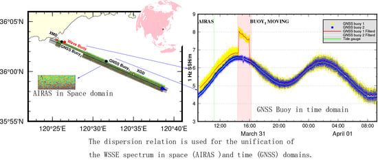
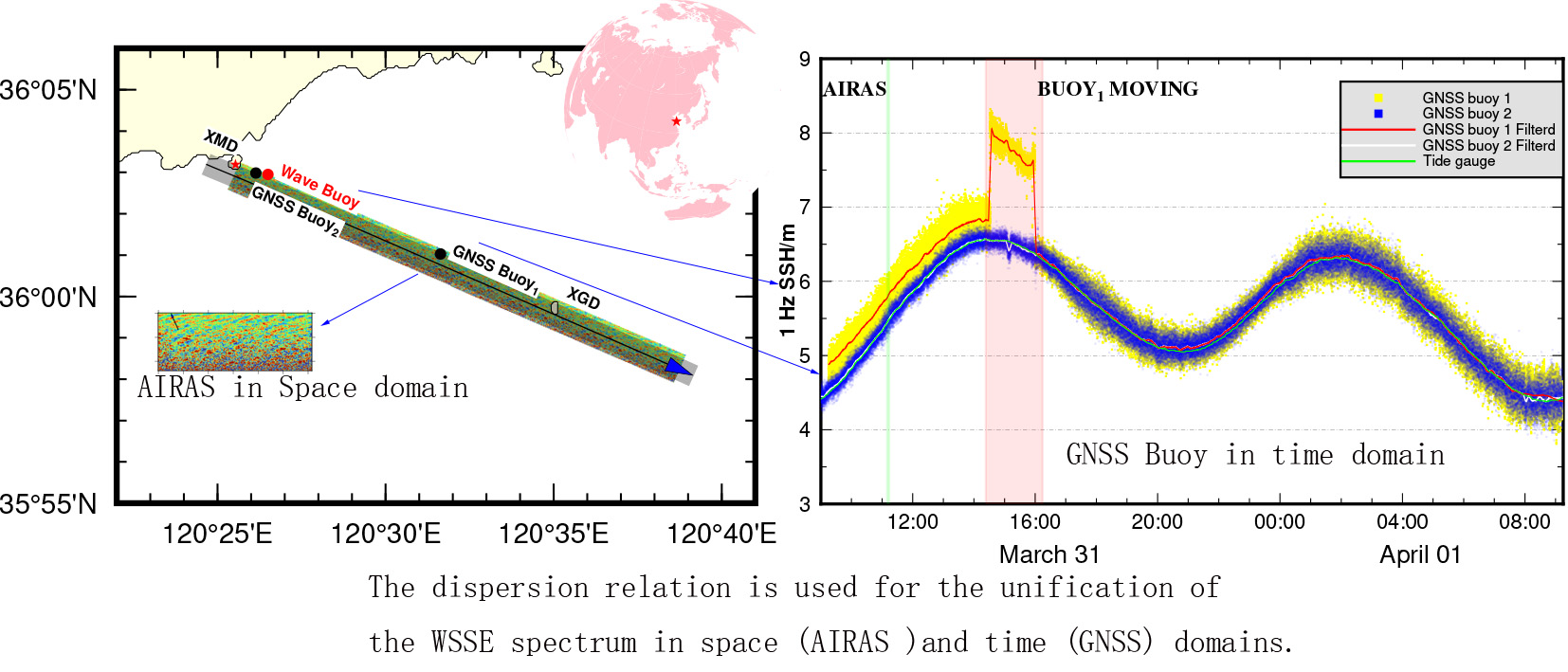
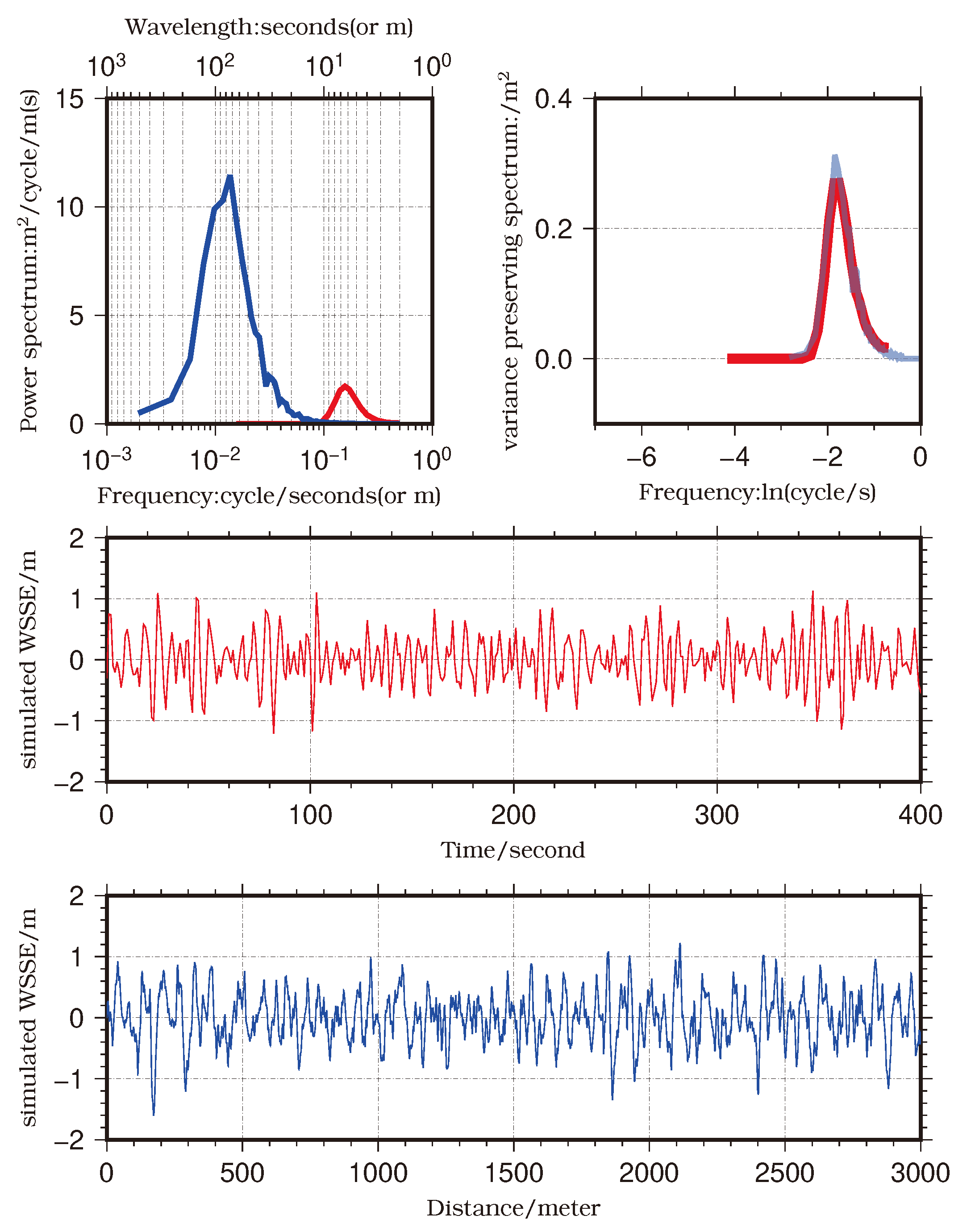
4.2. Validation of Wave-Induced Sea Surface Elevation

The WSSE is the dominant signal in the wavenumber or frequency domain of oceanic gravity waves [38]. We propose a validation method based on the assumption that the WSSE variance of an equilibrium wave field is uniform and can be measured equivalently in the space or time domains [44,45,46]. Specifically, for an equilibrium WSSE field, the following three statements can be made.

(1)

If the time series of the measured sea surface elevation is sufficiently long, the variance of the sea surface elevation measured at any place within the domain is the same (i.e., no place is different).

(2)

If the area of the measured sea surface elevation is sufficiently large, the variance of the sea surface elevation measured at any time within the domain is the same (i.e., no time is different).

(3)

If statements (1) and (2) are true, the WSSE is a uniform field in space and time, and the variances of (1) and (2) are equal.

The power spectrum density (PSD) of the WSSE signal has been proven a useful indicator in the Cal/Val of interferometric altimeters owing to its relation to the dynamics of the ocean interior [33]. The PSD can be used to estimate not only the WSSE variance but also the distributions of variance in wavenumber/frequency bands. In this investigation, we use the PSD to conduct the validation. The methods used for calculating the PSD and related settings are detailed in Appendix A. Based on statements of (1)–(3), the sea surface elevation variances in the space and time domains could be expressed as the integral of the PSD over the wavenumber/frequency bands:

$${\sigma }^2={\int }_{f_0}^{f_n}S\left(f\right)df={\int }_{k_0}^{k_n}Q\left(k\right)dk,$$

(2)

where ${\sigma }^2$ is the variance, f and k are the frequency and wavenumber in the time and space domains, respectively, and S and Q represent the power spectrum density in the time and space domains, respectively. Therefore, we could use the WSSE measured in the time domain by the GNSS buoys to validate the AIRAS in the space domain.

The variance distributions of the WSSE in the time and space domains could not be compared directly because they are expressed in different units and scales. To assess the consistency of the PSD shapes of the WSSE in the time/space domains, we first needed them to be unified. To show the fraction of variance in one band relative to other bands, the variance-preserving spectrum (VPS; the variance is not changed during the transform) could be calculated using the following mathematical transform based on Equation (2) [47]:

$${\sigma }^2={\int }_{f_0}^{f_n}fS\left(f\right)d\left(ln\left(f\right)\right)={\int }_{k_0}^{k_n}kQ\left(k\right)d\left(ln\left(k\right)\right).$$

(3)

The dispersion relation of gravity waves in deep water is then used for the PSD conversion between the space domain and the time domain:

$$k=\frac{{\left(2\pi f\right)}^2}{g},$$

(4)

where g is gravitational acceleration, k is the wavenumber, and f is the ocean wave frequency. Based on the theoretical dispersion relation (Equation (4)) and the VPS (Equation (3)), the relation between the VPS in terms of the frequency and the wavenumber domains could be expressed as (Appendix B):

$$\begin{array}{cc}\hfill d\left(ln\right(f\left)\right)& =\frac{1}{2}·d\left(ln\right(k\left)\right),\hfill \\ \hfill S\left(f\right)f& =2·Q\left(k\right)k.\hfill \end{array}$$

(5)

Finally, the variance as well as the variance (or power) distribution of the AIRAS WSSE could be validated using the GNSS buoys data. In this study, the variance was estimated using the integral of the PSD (or VPS) over the frequency/wavenumber domain, which neglects those signals outside the maximum and minimum bands of the frequency/wavenumber. For the measured WSSE from the GNSS data and the AIRAS, the difference between their unified VPSs arises mainly from measurement errors, and the integral of the difference of the two VPSs gives the total variance of the error in the wave frequency/wavenumber bands. Moreover, the difference in the VPS shapes could reflect the error of the power at different frequencies or wavenumbers. The correlation coefficient can be used to assess the consistency of the unified VPS shapes.

5. Results

For assessment of the AIRAS data, the validation is based on the relative SSH difference and the WSSE spectra. For the relative SSH signals, we compare the SSH differences of the GNSS buoys and the AIRAS at different locations directly. For the WSSE spectra, the PSD methods proposed in Section 4 are employed. To test the feasibility of the spectra method, we first applied it to the simulated WSSE.

5.1. Simulated WSSE

For this study, the Pierson–Moskowitz wave spectrum, which is a widely accepted relationship that defines the distribution of wave energy with respect to frequency, was used to generate the simulated WSSE under the developed wind-generated seas [36]. First, the time series of the WSSE, deemed the GNSS buoy measurements, was simulated at one fixed point on the ocean as the sum of a large number of wave components at different frequencies. Then, at a specific time, the two-dimensional WSSE in the space domain was generated (Figure 10). The WSSE of the time and space series, the PSD over the wavenumber and frequency domains, and the unified VPS in the time domain are shown in Figure 11.

By integrating the power density over the wavenumber/frequency domains, the variances of the WSSE were estimated as $0.188$ and $0.186$ m² (i.e., nearly the same), respectively. The PSDs of the time and space WSSE series, shown in the upper-left image of Figure 11, are illustrated with different units on the x and y axes for the different domains. Thus, the shape and the amplitude of the PSD curves are markedly different even though they yield the same variance. After applying the transform through Equation (5), as illustrated in the upper-right image of Figure 11, the PSD curve of the WSSE in the space domain is converted to the VPS in the time domain. Thus, the shape and the area of the spectrum in the time and space domains could be compared directly. The VPSs from the space and time domains fit almost perfectly, including the area under the curves and the shape of the curves. This suggests that the proposed method of validation of spectral analysis is reasonable. Therefore, the difference of the VPSs can be used to evaluate the measurement errors in the AIRAS experiment.

5.2. Sea Surface Height Difference Between Validation Locations

The SSHs derived from both the GNSS buoys and the AIRAS were defined with respect to the WGS-84 ellipsoid. Thus, the relative SSH of the AIRAS could be assessed using the GNSS buoy measurements. The SSH difference from the two GNSS buoys was $30\pm 1$ cm after correction for local tides estimated using the regional NAO99jb tidal model and removal of the WSSE signals through application of the low-pass filter. The tidal correction could not be neglected because it could have reached as high as 5 cm during the experimental period (see Figure 9).

To minimize the influence of waves on the AIRAS SSH, the SSH from the AIRAS was an average over an area of $480\times 240$ m centered over the two GNSS buoys. After adding the tide correction, the average SSH over the selected boxes was calculated. The mean SSH difference of the AIRAS between the locations of GNSS buoy 2 and buoy 1 was estimated as 27 cm. The AIRAS result is in good agreement with that obtained from the GNSS buoys, as well as the MSS models [42], as shown in

Table 2. The Cal/Val result of relative SSH difference of the AIRAS. The SSH difference was estimated between GNSS buoy 1 and buoy 2, which were 9 km apart.

Source	SSH Difference	Standard Deviation
GNSS buoys	30 cm	$\pm 1$ cm
AIRAS	27 cm	NaN
DTU MSS 2018 model	27 cm	NaN

. In comparison with the GNSS result, the AIRAS bias is less than 3 cm, which matches the designed parameters of the AIRAS.

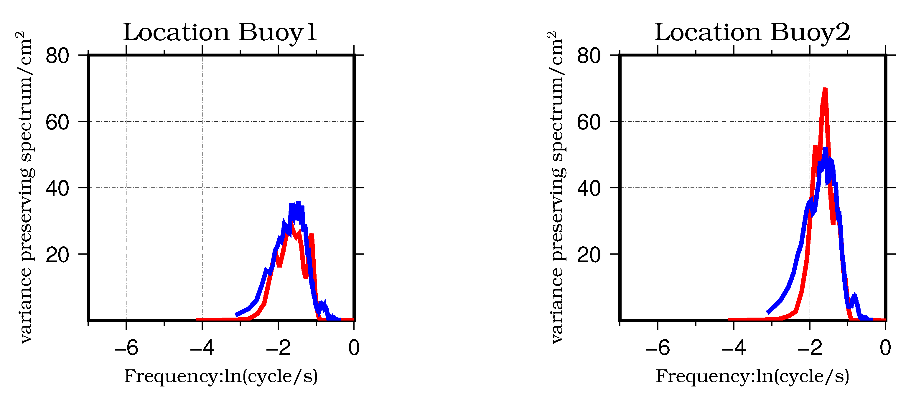
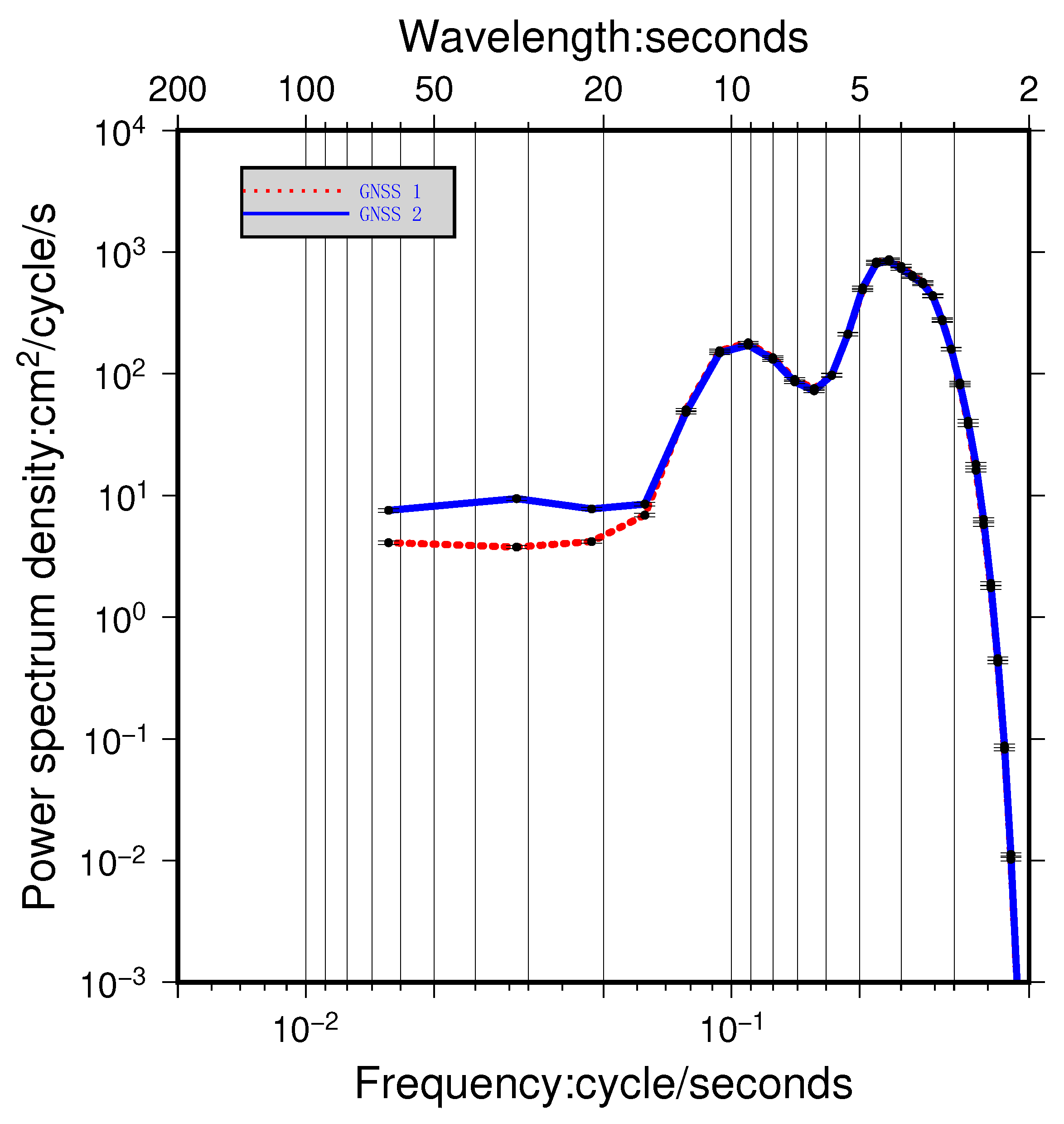
5.3. Spectrum Validation of the Wave-Induced Sea Surface Elevation

The WSSE is the dominant signal of the GNSS and AIRAS measurements in the space and time range of gravity waves. The WSSE could be expressed in the time domain and evaluated using the GNSS buoys or expressed in the space domain and evaluated using the AIRAS observations. Based on the discussion in Section 4.2 and the simulated WSSE described in Section 5.1, for an equilibrium wave field, the VPSs from the space and time domains fit almost perfectly, and therefore the difference of the VPSs can be used to evaluate the measurement errors in the AIRAS experiment.

For the WSSEs measured by the GNSS buoys in the time domain and by the AIRAS in the space domain, we first removed the linear trend and applied a low-pass filter to remove noise. For the AIRAS data, a low-pass filter was implemented to remove noise at wavelengths shorter than 3 m (see Figure 5) [48]. To make the AIRAS data comparable with the GNSS data, we sampled the AIRAS two-dimensional WSSE to one dimension along the direction of wave propagation before calculating the spectrum of the AIRAS data.

The PSD of the WSSE for the GNSS buoys and the AIRAS were calculated using same procedures (Appendix A). The unified VPS curves of the AIRAS and GNSS buoys are illustrated in Figure 12. The VPSs from both GNSS buoys show satisfactory consistency with that of the AIRAS. The correlation coefficient between the VPS of the AIRAS and that of GNSS buoy 1 is estimated as 0.90 and the difference of the integral variances is 8 cm²; the corresponding values for GNSS buoy 2 were 0.91 and 7 cm², respectively. The results indicate that the variance difference between the AIRAS and the GNSS buoys is less than 8 cm². Therefore, it could serve as a reference for the WSSE error over the scale range of waves (3–150 m). The variance distribution between them is similar, with a correlation coefficient higher than 0.90, indicating that the error is small relative to the WSSE signal. The statistical Cal/Val results of the WSSE measured using the AIRAS are given in

Table 3. The Cal/Val result of the AIRAS measured WSSE. Variance was estimated from the VPSs of the GNSS buoys and the AIRAS WSSE.

Location	Source	Variance	Bias	Correlation Coefficient
GNSS Buoy 1	GNSS	28 cm${}^2$	8 cm${}^2$	$0.90$
	AIRAS	36 cm${}^2$
GNSS buoy 2	GNSS	45 cm${}^2$	7 cm${}^2$	$0.91$
	AIRAS	52 cm${}^2$

.

6. Conclusions and Discussion

The Cal/Val of interferometric altimeters is an essential, challenging, and compelling task because of the launches of the SWOT and Guanlan satellites planned for the near future. We proposed a Cal/Val method based on the assumption that the WSSE variance of an equilibrium wave field is uniform and that equivalent measurements can be made in the time or space domains. Here, we took advantage of the dispersion relation and linked the power spectrum density of the WSSE in the space domain to the time domain, which is much easier for in situ facilities to measure. Using simulated data, this approach was proven feasible. For the case study over a sea area off the coast of Qingdao (China), we applied the proposed method to the Cal/Val of the AIRAS airborne swath interferometric altimeter using GNSS buoy data.

Results indicate that the differences of the WSSE variances from the AIRAS and the two GNSS buoys were below 8 cm², corresponding to a standard deviation of 2.8 cm. Therefore, it could serve as a reference for the WSSE error over the scale range of waves. The correlation coefficient between the AIRAS and GNSS buoys was approximately 0.90, indicating that the error was small relative to the WSSE signal. As for the difference in SSH measurements, our analysis showed that the AIRAS has satisfactory consistency with two GNSS buoys that were separated by a distance of 9 km, i.e., the difference was 3 cm. The bias of the AIRAS SSH could satisfy the expected uncertainty of 3.4 cm.

Our research is based on the statement that the WSSE variance of an equilibrium wave field is uniform and that it could be measured equivalently in the space or time domains. However, the spatial resolutions and coverages of the sensors of the SWOT and Guanlan satellite missions are markedly different to those of the airborne interferometric altimeter. Therefore, the applicability of the proposed approach to instruments onboard spaceborne platforms requires further investigation. Here, we mainly proved the feasibility of using GNSS buoys to assess airborne interferometric altimeter data. We also emphasize that our campaign was conducted under the conditions of a calm sea state in which the SWH was 20–30 cm. However, under different sea states, particularly in harsh conditions, the performance of the AIRAS will need further study. In addition, the main aim of interferometric radar altimeters is to measure the submesoscale ocean processes and the ocean wave is usually regarded as a error budget that could perturb the submesoscale signals, so the GNSS buoy and the AIRAS data may be useful for better estimating the SSH error budget owing to the wind-induced waves.

The results of this study represent the first evaluation of the ability of the AIRAS to measure two-dimensional WSSEs and SSH differences. The proposed Cal/Val method provides a perspective for future spaceborne or airborne interferometric altimeters. Our subsequent work will seek to verify the feasibility of this method by conducting additional experimentation under different sea conditions.

References

1. Fu, L.L.; Haines, B.J. The challenges in long-term altimetry calibration for addressing the problem of global sea level change. Adv. Space Res. 2013, 51, 1284–1300. [Google Scholar] [CrossRef]
2. Haines, B.J.; Desai, S.D.; Born, G.H. The Harvest Experiment: Calibration of the Climate Data Record from TOPEX/Poseidon, Jason-1 and the Ocean Surface Topography Mission. Mar. Geod. 2010, 33, 91–113. [Google Scholar] [CrossRef]
3. Haines, B.J.; Dong, D.; Born, G.H.; Gill, S.K. The Harvest Experiment: Monitoring Jason-1 and TOPEX/POSEIDON from a California Offshore Platform Special Issue: Jason-1 Calibration/Validation. Mar. Geod. 2003, 26, 239–259. [Google Scholar] [CrossRef]
4. Ménard, Y.; Jeansou, E.; Vincent, P. Calibration of the TOPEX/POSEIDON altimeters at Lampedusa: Additional results at Harvest. J. Geophys. Res. Ocean. (1978–2012) 1994, 99, 24487–24504. [Google Scholar] [CrossRef]
5. Christensen, E.J.; Haines, B.J.; Keihm, S.J.; Morris, C.S.; Norman, R.A.; Purcell, G.H.; Williams, B.G.; Wilson, B.D.; Born, G.H.; Parke, M.E.; et al. Calibration of TOPEX/POSEIDON at Platform Harvest. J. Geophys. Res. Ocean. 1994, 99, 24465–24485. [Google Scholar] [CrossRef]
6. Bonnefond, P.; Laurain, O.; Exertier, P.; Boy, F.; Guinle, T.; Picot, N.; Labroue, S.; Raynal, M.; Donlon, C.; Féménias, P.; et al. Calibrating the SAR SSH of Sentinel-3A and CryoSat-2 over the Corsica Facilities. Remote Sens. 2018, 10, 92. [Google Scholar] [CrossRef] [Green Version]
7. Bonnefond, P.; Exertier, P.; Laurain, O.; Ménard, Y.; Orsoni, A.; Jeansou, E.; Haines, B.J.; Kubitschek, D.G.; Born, G. Leveling the Sea Surface Using a GPS-Catamaran Special Issue: Jason-1 Calibration/Validation. Mar. Geod. 2003, 26, 319–334. [Google Scholar] [CrossRef]
8. Bonnefond, P.; Exertier, P.; Laurain, O.; Guillot, A.; Picot, N.; Cancet, M.; Lyard, F. SARAL/AltiKa Absolute Calibration from the Multi-Mission Corsica Facilities. Mar. Geod. 2015, 38, 171–192. [Google Scholar] [CrossRef] [Green Version]
9. Bonnefond, P.; Exertier, P.; Laurain, O.; Jan, G. Absolute calibration of Jason-1 and Jason-2 altimeters in Corsica during the formation flight phase. Mar. Geod. 2010, 33, 80–90. [Google Scholar] [CrossRef]
10. Bonnefond, P.; Exertier, P.; Laurain, O.; Ménard, Y.; Orsoni, A.; Jan, G.; Jeansou, E. Absolute Calibration of Jason-1 and TOPEX/Poseidon Altimeters in Corsica Special Issue: Jason-1 Calibration/Validation. Mar. Geod. 2003, 26, 261–284. [Google Scholar] [CrossRef]
11. Mertikas, S.; Donlon, C.; Féménias, P.; Mavrocordatos, C.; Galanakis, D.; Tripolitsiotis, A.; Frantzis, X.; Kokolakis, C.; Tziavos, I.N.; Vergos, G.; et al. Absolute Calibration of the European Sentinel-3A Surface Topography Mission over the Permanent Facility for Altimetry Calibration in west Crete, Greece. Remote Sens. 2018, 10, 1808. [Google Scholar] [CrossRef] [Green Version]
12. Mertikas, S.P.; Donlon, G.; Vuilleumier, P.; Cullen, R.; Féménias, P.; Tripolitsiotis, A. An Action Plan Towards Fiducial Reference Measurements for Satellite Altimetry. Remote Sens. 2019, 11, 1993. [Google Scholar] [CrossRef] [Green Version]
13. Mertikas, S.P.; Donlon, C.; Féménias, P.; Mavrocordatos, C.; Galanakis, D.; Tripolitsiotis, A.; Frantzis, X.; Tziavos, I.N.; Vergos, G.; Guinle, T. Fifteen Years of Cal/Val Service to Reference Altimetry Missions: Calibration of Satellite Altimetry at the Permanent Facilities in Gavdos and Crete, Greece. Remote Sens. 2018, 10, 1557. [Google Scholar] [CrossRef] [Green Version]
14. Watson, C.; White, N.; Church, J.; Burgette, R.; Tregoning, P.; Coleman, R. Absolute Calibration in Bass Strait, Australia: TOPEX, Jason-1 and OSTM/Jason-2. Mar. Geod. 2011, 34, 242–260. [Google Scholar] [CrossRef]
15. Watson, C.; Coleman, R.; White, N.; Church, J.; Govind, R. Absolute Calibration of TOPEX/Poseidon and Jason-1 Using GPS Buoys in Bass Strait, Australia Special Issue: Jason-1 Calibration/Validation. Mar. Geod. 2003, 26, 285–304. [Google Scholar] [CrossRef]
16. Watson, C.; White, N.; Coleman, R.; Church, J.; Morgan, P.; Govind, R. TOPEX/Poseidon and Jason-1: Absolute Calibration in Bass Strait, Australia. Mar. Geod. 2004, 27, 107–131. [Google Scholar] [CrossRef]
17. Yang, L.; Zhou, X.; Mertikas, S.P.; Zhu, L.; Yang, L.; Lei, N. First Calibration Results of Jason-2 and Saral/AltiKa Satellite Altimeters from the Qianliyan Permanent Facilities. Adv. Space Res. 2017, 59, 2831–2842. [Google Scholar] [CrossRef]
18. Zhou, X.; Yang, L.; Wang, Y.; Zhu, L.; Fu, Y.; Li, F. Research Progress of Satellite Altimeter Calibration in China. In Proceedings of the IGARSS 2019—2019 IEEE International Geoscience and Remote Sensing Symposium, Yokohama, Japan, 28 July–2 August 2019; pp. 8297–8299. [Google Scholar] [CrossRef]
19. Lei, Y.; Xinghua, Z.; Quanjun, X.; Baogui, K.; Bo, M.; Lin, Z. Research status of satellite altimeter calibration. J. Remote Sens. 2019, 23, 392–407. [Google Scholar] [CrossRef]
20. Crétaux, J.F.; Bergé-Nguyen, M.; Calmant, S.; Jamangulova, N.; Satylkanov, R.; Lyard, F.; Perosanz, F.; Verron, J.; Samine Montazem, A.; Le Guilcher, G.; et al. Absolute Calibration or Validation of the Altimeters on the Sentinel-3A and the Jason-3 over Lake Issykkul (Kyrgyzstan). Remote Sens. 2018, 10, 1679. [Google Scholar] [CrossRef] [Green Version]
21. Crétaux, J.F.; Calmant, S.; Romanovski, V.; Perosanz, F.; Tashbaeva, S.; Bonnefond, P.; Moreira, D.; Shum, C.; Nino, F.; Bergé-Nguyen, M. Absolute calibration of Jason radar altimeters from GPS kinematic campaigns over Lake Issykkul. Mar. Geod. 2011, 34, 291–318. [Google Scholar] [CrossRef]
22. Crétaux, J.F.; Calmant, S.; Romanovski, V.; Shabunin, A.; Lyard, F.; Bergé-Nguyen, M.; Cazenave, A.; Hernandez, F.; Perosanz, F. An absolute calibration site for radar altimeters in the continental domain: Lake Issykkul in Central Asia. J. Geod. 2008, 83, 723–735. [Google Scholar] [CrossRef]
23. Shum, C.; Yi, Y.; Cheng, K.; Kuo, C.; Braun, A.; Calmant, S.; Chambers, D. Calibration of JASON-1 Altimeter over Lake Erie Special Issue: Jason-1 Calibration/Validation. Mar. Geod. 2003, 26, 335–354. [Google Scholar] [CrossRef]
24. Dong, X.; Woodworth, P.; Moore, P.; Bingley, R. Absolute Calibration of the TOPEX/POSEIDON Altimeters using UK Tide Gauges, GPS, and Precise, Local Geoid-Differences. Mar. Geod. 2002, 25, 189–204. [Google Scholar] [CrossRef]
25. Chen, G.; Tang, J.; Zhao, C.; Wu, S.; Yu, F.; Ma, C.; Xu, Y.; Chen, W.; Zhang, Y.; Liu, J.; et al. Concept Design of the “Guanlan” Science Mission: China’s Novel Contribution to Space Oceanography. Front. Mar. Sci. 2019, 6, 194. [Google Scholar] [CrossRef] [Green Version]
26. Fu, L.L.; Ubelmann, C. On the Transition from Profile Altimeter to Swath Altimeter for Observing Global Ocean Surface Topography. J. Atmos. Ocean. Technol. 2014, 31, 560–568. [Google Scholar] [CrossRef]
27. Wang, J.; Fu, L.L.; Torres, H.S.; Chen, S.; Qiu, B.; Menemenlis, D. On the Spatial Scales to be Resolved by the Surface Water and Ocean Topography Ka-Band Radar Interferometer. J. Atmos. Ocean. Technol. 2019, 36, 87–99. [Google Scholar] [CrossRef] [Green Version]
28. Morrow, R.; Fu, L.L.; Ardhuin, F.; Benkiran, M.; Chapron, B.; Cosme, E.; d’Ovidio, F.; Farrar, J.T.; Gille, S.T.; Lapeyre, G.; et al. Global Observations of Fine-Scale Ocean Surface Topography With the Surface Water and Ocean Topography (SWOT) Mission. Front. Mar. Sci. 2019, 6, 232. [Google Scholar] [CrossRef]
29. Wang, J.; Fu, L.L. On the Long-Wavelength Validation of the SWOT KaRIn Measurement. J. Atmos. Ocean. Technol. 2019, 36, 843–848. [Google Scholar] [CrossRef]
30. Daniel, E.F. SWOT Project Mission Performance and Error Budget Revision A; Technical Report JPL D-79084; NASA/JPL: Pasadena, CA, USA, 2017.
31. Altenau, E.H.; Pavelsky, T.M.; Moller, D.; Lion, C.; Pitcher, L.H.; Allen, G.H.; Bates, P.D.; Calmant, S.; Durand, M.; Smith, L.C. AirSWOT measurements of river water surface elevation and slope: Tanana River, AK. Geophys. Res. Lett. 2017, 44, 181–189. [Google Scholar] [CrossRef] [Green Version]
32. Tuozzolo, S.; Lind, G.; Overstreet, B.; Mangano, J.; Fonstad, M.; Hagemann, M.; Frasson, R.P.M.; Larnier, K.; Garambois, P.A.; Monnier, J.; et al. Estimating River Discharge with Swath Altimetry: A Proof of Concept Using AirSWOT Observations. Geophys. Res. Lett. 2019, 46, 1459–1466. [Google Scholar] [CrossRef]
33. Wang, J.; Fu, L.L.; Qiu, B.; Menemenlis, D.; Farrar, J.T.; Chao, Y.; Thompson, A.F.; Flexas, M.M. An Observing System Simulation Experiment for the Calibration and Validation of the Surface Water Ocean Topography Sea Surface Height Measurement Using In Situ Platforms. J. Atmos. Ocean. Technol. 2017, 35, 281–297. [Google Scholar] [CrossRef]
34. Li, Z.; Wang, J.; Fu, L.L. An Observing System Simulation Experiment for Ocean State Estimation to Assess the Performance of the SWOT Mission: Part 1—A Twin Experiment. J. Geophys. Res. Ocean. 2019, 124, 4838–4855. [Google Scholar] [CrossRef]
35. Zhang, Y.; Shi, X.; Wang, H.; Tan, Y.; Zhai, W.; Dong, X.; Kang, X.; Yang, Q.; Li, D.; Jiang, J. Interferometric Imaging Radar Altimeter on Board Chinese Tiangong-2 Space Laboratory. In Proceedings of the 2018 Asia-Pacific Microwave Conference (APMC), Kyoto, Japan, 6–9 November 2018; pp. 851–853. [Google Scholar] [CrossRef]
36. Alves, J.H.G.M.; Banner, M.L.; Young, I.R. Revisiting the Pierson–Moskowitz Asymptotic Limits for Fully Developed Wind Waves. J. Phys. Oceanogr. 2003, 33, 1301–1323. [Google Scholar] [CrossRef]
37. Rodriguez, E.; Martin, J. Theory and design of interferometric synthetic aperture radars. IEE Proc. F Radar Signal Process. 1992, 139, 147–159. [Google Scholar] [CrossRef]
38. Toffoli, A.; Bitner-Gregersen, E.M. Types of Ocean Surface Waves, Wave Classification. In Encyclopedia of Maritime and Offshore Engineering; John Wiley & Sons, Ltd.: Hoboken, NJ, USA, 2017; pp. 1–8. [Google Scholar] [CrossRef]
39. Lin, Y. Development and Applications of A GNSS Buoy for Monitoring tides and Ocean Waves in Coastal Areas. Ph.D. Thesis, National Cheng Kung University, Tainan, Taiwan, 2018. [Google Scholar]
40. Herring, T.; King, R.; McClusky, S. GAMIT Reference Manual, GPS Analysis at MIT, Release 10.4.; Massachusetts Institute of Technology: Cambridge, MA, USA, 2010. [Google Scholar]
41. Matsumoto, K.; Takanezawa, T.; Ooe, M. Ocean Tide Models Developed by Assimilating TOPEX/POSEIDON Altimeter Data into Hydrodynamical Model: A Global Model and a Regional Model around Japan. J. Oceanogr. 2000, 56, 567–581. [Google Scholar] [CrossRef]
42. Andersen, O.; Knudsen, P.; Stenseng, L. The DTU13 MSS (Mean Sea Surface) and MDT (Mean Dynamic Topography) from 20 Years of Satellite Altimetry. In IGFS 2014; Jin, S., Barzaghi, R., Eds.; Springer International Publishing: Cham, Switzerland, 2016; pp. 111–121. [Google Scholar]
43. Martinez-Benjamin, J.J.; Martinez-Garcia, M.; Lopez, S.G.; Andres, A.N.; Pozuelo, F.B.; Infantes, M.E.; Lopez-Marco, J.; Davila, J.M.; Pasquin, J.G.; Silva, C.G.; et al. Ibiza Absolute Calibration Experiment: Survey and Preliminary Results. Marine Geodesy 2004, 27, 657–681. [Google Scholar] [CrossRef]
44. Rikka, S.; Uiboupin, R.; Kõuts, T.; Vahter, K.; Pärt, S. A Method for Significant Wave Height Estimation from Circularly Polarized X-Band Coastal Marine Radar Images. IEEE Geosci. Remote Sens. Lett. 2019, 16, 844–848. [Google Scholar] [CrossRef]
45. Populus, J.; Aristaghes, C.; Jonsson, L.; Augustin, J.; Pouliquen, E. The use of SPOT data for wave analysis. Remote Sens. Environ. 1991, 36, 55–65. [Google Scholar] [CrossRef]
46. Salin, B.M.; Salin, M.B. Combined Method for Measuring 3D Wave Spectra. II. Examples of Using the Basic Measurement Procedures and Analysis of the Obtained Results. Radiophys. Quantum Electron. 2015, 58, 185–196. [Google Scholar] [CrossRef]
47. Emery, W.J.; Thomson, R.E. Data Analysis Methods in Physical Oceanography; Elsevier Science: Amsterdam, The Netherlands, 1998. [Google Scholar]
48. Qiufu, J.; Yongsheng, X.; Hanwei, S.; Lideng, W.; Lei, Y. Ocean Surface Waves Observation from Airborne Ka band Interferometric Altimeter. Remote Sens. 2020. submitted. [Google Scholar]
49. Wessel, P.; Smith, W.H.F.; Scharroo, R.; Luis, J.; Wobbe, F. Generic Mapping Tools: Improved Version Released. Eos Trans. Am. Geophys. Union 2013, 94, 409–410. [Google Scholar] [CrossRef] [Green Version]
50. Welch, P.D. The use of fast Fourier transform for the estimation of power spectra: A method based on time averaging over short, modified periodograms. IEEE Trans. Audio Electroacoust. 1967, 15, 70–73. [Google Scholar] [CrossRef] [Green Version]
51. Percival, D.B.; Walden, A.T. Spectral Analysis for Physical Applications; Cambridge University Press: Cambridge, UK, 1993. [Google Scholar] [CrossRef]
Figure 1. Map of the AIRAS experiment area around the station XMD, Qingdao, China. GNSS buoy 1 and buoy 2 were deployed at sea, separated by a distance of 9 km. Buoy 1 was moved to the location of buoy 2 after the AIRAS campaign was completed to cross validate the measurements of the GNSS buoys and tide gauges.
Remotesensing 12 01651 g001
Figure 2. The mean sea surface (MSS) and mean dynamic topography (MDT) models over the campaign sea area. Black points represent the GNSS buoy locations; the black line represents the flight path.
Remotesensing 12 01651 g002
Figure 3. Principles of height measurement using an interferometric imaging altimeter.
Remotesensing 12 01651 g003
Figure 4. Flowchart of data processing for determining sea surface heights using the AIRAS.
Remotesensing 12 01651 g004
Figure 5. The relative sea surface elevation measured by the AIRAS. The right-hand panels show the unfiltered AIRAS data; the left-hand panels show the band-pass filtered AIRAS data (3–150 m). The arrows in the left-hand images represent the direction of wave propagation. The X-axis is the direction of AIRAS flight and the Y-axis is the cross-track direction.
Remotesensing 12 01651 g005
Figure 6. The spirit leveling work between the GNSS permanent station and the tide gauge at station XMD. The left-hand photo is of the permanent GNSS station; the middle photo shows the leveling work between the GNSS and the benchmark of the tide gauge; and the right-hand photo shows the benchmark of the tide gauge and the tide station.
Remotesensing 12 01651 g006
Figure 7. The GNSS buoys tethered at the same location close to the station XMD tide gauge for cross-validation purposes.
Remotesensing 12 01651 g007
Figure 8. Sea surface heights (SSHs) retrieved from GNSS buoys and in situ tide gauge data. The AIRAS campaign was conducted from 09:00 local time (LT) on 31 March 2019 to 14:00 LT on 31 March 2019. The AIRAS data used in this investigation were collected at approximately 11:00 LT. During 14:20–16:00 LT, GNSS buoy 1 was transported by ship to the location of buoy 2.
Remotesensing 12 01651 g008
Figure 9. Sea surface height (SSH) difference between GNSS buoy 1 and buoy 2 (expressed as G1-G2), and the SSH difference between GNSS buoy2 and the tide gauge (expressed as G2-TG). The yellow lines represent the SSH differences without the correction of the NAO99jb tide model.
Remotesensing 12 01651 g009
Figure 10. Simulated two-dimensional WSSE using the Pierson–Moskowitz spectrum.
Remotesensing 12 01651 g010
Figure 11. Simulated WSSE and its associated spectrum. The red (blue) line is the WSSE series in the time (space) domain. The upper-left image presents the nonunified PSD in the time/space domains. The upper-right image shows the unified VPS in the time domain.
Remotesensing 12 01651 g011
Figure 12. Unified VPS in frequency domain of WSSE measured by AIRAS and GNSS buoys. Red (blue) line represents the GNSS buoy (AIRAS) data.
Remotesensing 12 01651 g012