Article

A Neural Network-Based Rain Effect Correction Method for HY-2A Scatterometer Backscatter Measurements

1
School of Geographical Sciences, Guangzhou University, Guangzhou 510006, China
2
School of Geography and Planning, Sun Yat-Sen University, Guangzhou 510275, China
3
National Satellite Ocean Application Service, Beijing 100081, China
*
Author to whom correspondence should be addressed.
Remote Sens. 2020, 12(10), 1648; https://doi.org/10.3390/rs12101648
Submission received: 24 April 2020 / Revised: 15 May 2020 / Accepted: 19 May 2020 / Published: 21 May 2020
(This article belongs to the Section Ocean Remote Sensing)

Abstract

:
The backscattering coefficients measured by Ku-band scatterometers are strongly affected by rainfall, resulting in a systematic error in sea surface wind field retrieval. In rainy conditions, the radar signals are subject to absorption by the raindrops in their round-trip propagation through the atmosphere, while the backscatter of raindrops raises the echo energy. In addition, raindrops give rise to roughness by impinging the ocean surface, resulting in an increase in the echo energy measured by a scatterometer. Under moderate wind conditions, the comprehensive impact of rainfall causes the wind speeds retrieved by the scatterometer to be higher than their actual values. The HY-2A scatterometer is a Ku-band, pencil-beam, conically scanning scatterometer. To correct the systematic error of the HY-2A scatterometer measurement in rainy conditions, a neural network model is proposed according to the characteristics of the backscatter coefficients measured by the HY-2A scatterometer in the presence of rain. With the neural network, the wind fields of the European Centre for Medium-range Weather Forecasts (ECMWF) reanalysis data were used as the reference to correct the deviation in backscatter coefficients measured by the HY-2A scatterometer in rainy conditions, and the accuracy in wind speeds retrieved using the corrected backscatter coefficients was significantly improved. Compared with the cases of wind retrieval without rain effect correction, the wind speeds retrieved from the corrected backscatter coefficients by the neural network show a much lower systematic deviation, which indicates that the neural network can effectively remove the systematic deviation in the backscatter coefficients and the retrieved wind speeds caused by rain.

Graphical Abstract

1. Introduction

The upper ocean dynamic environment is closely related to sea surface wind. Conventional sea surface wind measurement platforms, such as ships, marine buoys, and stations, all have deficiencies either in spatial coverage or in measurement accuracy, while satellite-borne scatterometers have a great advantage in obtaining large-scale, synchronous ocean surface winds. Generally, the operation wavelengths of the launched satellite-borne scatterometers is mainly in C (5.3 GHz) and Ku (13.5 GHz) bands. In 1978, the first satellite-borne scatterometer, named SASS (SeaSat Scatterometer), was successfully launched onboard the SeaSAT-A satellite and operated in the Ku-band. Afterwards, NASA (National Aeronautics and Space Administration) launched several more Ku-band scatterometers, including NSCAT, SeaWinds, and QuikScat. The typical representatives of the C-band satellite-borne scatterometers mainly include the AMI and ASCAT series, launched by the European Space Agency (ESA) and operated by the European Organisation for the Exploitation of Meteorological Satellites (EUMETSAT). The HY-2A scatterometer is the first operational space-borne scatterometer in China, and it is a Ku-band, pencil-beam, conically scanning scatterometer onboard the HY-2A satellite, an ocean dynamic remote sensing satellite, launched in August 2011.
The scatterometer makes it possible to acquire the sea surface wind through a quantitative relationship, which correlates the sea surface wind with the normalized radar backscatter cross section, also known as the backscatter coefficient (σ0). In scatterometry, such a relationship is termed the geophysical model function (GMF), which relates the radar backscatter coefficient to sea surface wind and radar parameters including incidence angle, azimuth angle, polarization, etc. The principle of wind field inversion is based on finding the wind speed and direction in the GMF, which are closest to the measured values of the backscatter coefficient. The main and most concerning problems in the process of measuring wind with a scatterometer include the GMF, the wind vector retrieval algorithm and the ambiguity or false solution removal. A geophysical model function for the X-band, based on a physical mechanism, was first proposed by Wright in 1966 [1]. Since then, many scholars have attempted to establish theoretical GMFs for microwave scatterometers. Due to insufficient knowledge of the interactive mechanism between microwaves and ocean wind, the theoretical analysis model based on physical mechanisms is incomplete and not sufficiently accurate for wind vector retrieval. Thus, semi-analytical models are more widely used in operational wind retrieval [2]. A semi-analytical model is a kind of GMF in which a functional relationship among the parameters is assumed and the model coefficients are determined by fitting methods. In practice, the measured wind data or numerical weather forecast wind data associated with the collocated radar backscatter coefficient data are usually used as input to establish a semi-analytical model. According to different radar instruments, researchers have established multiple semi-analytical GMFs, such as SASS-1, NSCAT-1, NSCAT-2, QSCAT-1, Ku-2001, and Ku-2011 for the Ku band and CMOD4, CMOD-IFR2, CMOD5, and CMOD7 for the C band [3,4,5]. The nonlinear characteristics of GMF make it difficult to directly calculate wind vector solutions from backscatter coefficients, and instrument noise also has an impact on wind retrieval from scatterometers. Aiming at the abovementioned problems, researchers have proposed a variety of scatterometer wind retrieval algorithms, such as the sum of square (SOS) algorithm and the maximum likelihood estimation (MLE) method. The MLE method is deemed an optimal algorithm due to its high performance and independence of GMF in the sea surface wind inversion of scatterometers [6]. In scatterometer wind inversion, multiple wind vector solutions are usually obtained for a wind vector cell (WVC), so an ambiguity removal procedure is needed to determine the unique wind field. Because the process of ambiguity removal should make best use of the information of the scatterometer data itself, the circular median filter algorithm is generally applied to remove the multiple ambiguities. The means of the wind field initialization before filtering determines the effect of the ambiguity removal. Researchers proposed choosing the solution with the maximum probability (the most likely solution) or the solution closest to the model predicted wind vector as the initial wind vector for each WVC [7,8]. Lin et al. proposed a multiple solution removal method for the SASS scatterometer and improved the performance of ambiguity removal in SASS data processing [9].
The microwave scatterometer can measure the backscatter coefficients under varied weather conditions. The backscatter coefficients measured by the scatterometer have a high accuracy in rain-free conditions; however, in the case of rain, the microwave echo energy received by the scatterometer is altered by the comprehensive effect of raindrops, resulting in a significant decrease in the wind retrieval accuracy. This effect of rain is particularly obvious in the event of a hurricane or typhoon [10]. The scatterometer-observed data contaminated by rain are estimated to account for 4–10%. Although rain identification and flagging technology have intensively been investigated, the impact and correction of rain is not taken into account in the current operational wind field retrieval. The factors altering the backscatter coefficients include not only the sea surface roughness caused by wind but also the impact of rain. The main effect of rain on wind field inversion is to change the radar backscatter energy received by the scatterometer [11]. When raindrops fall into the ocean surface, the splashing effect and the generated ring waves will affect the scattering of the ocean surface. Generally, the splashing of raindrops will enhance the roughness of the sea surface, which, in turn, enhances the radar backscatter energy. In addition, the microwave signals of the scatterometer are partly scattered and absorbed by raindrops when passing though the atmosphere under rainy conditions. The effect of the backscatter of raindrops causes an increase in the radar signal, while the effect of absorption of raindrops results in an attenuation of the radar signal [12,13].
Previously, multiple scholars have carried out in-depth research on the impact of rain, but the mechanism of the impact of rain is complicated and has not been fully investigated [14]. Weissman et al. developed empirical relations that show the errors in SeaWinds scatterometer wind magnitude induced by rainfall [15]. Nielsen et al. used AMSR data and SeaWinds data to establish a backscatter model of sea surface and rainfall impact [16]. Allen and Long proposed a new method that estimated both wind and rain from rain-contaminated measurements and applied the estimates to Ku-band scatterometer SeaWinds. Tropical rain measuring mission data were used as validation in the research [17]. Stiles et al. used a neural network wind speed correction model to improve the accuracy of the wind field retrieval of SeaWinds under rainy conditions [18]. Gohil et al. developed a method for rain flagging using a Ku band Oceansat-2 scatterometer to measure radar backscatter and noise-equivalent brightness temperature to detect the presence of rain [19]. Lin et al. addressed the quality control method for the C-band scatterometer ASCAT, and presented a rain flagging algorithm by employing the method of image processing, which is known as singularity analysis (SA) [20]. Owen and Long designed resolution enhancement algorithms for QuikSCAT that allow scatterometers to measure the higher resolution wind vector and identified much smaller rain events and their effects on the wind field [21]. Li et al. established a physical model according to the radiation equation of electromagnetic wave propagation in raindrops [22]. In this study involving the HY-2A scatterometer, we attempt to build a neural network model for backscatter coefficient correction under rainy conditions to reduce the systematic error in the backscatter coefficients and in the retrieved wind speeds. The experimental results indicate that this model can effectively correct the systematic errors in the backscatter coefficients caused by rain, leading to a higher wind retrieval accuracy than that without rain effect correction.
The rest of this article is organized as follows. In Section 2, we introduce the datasets used in this paper to build the neural network model and to perform the model validation, which mainly include the Level 2A data of the HY-2A scatterometer, TAO buoy data, ECMWF reanalysis wind field data, and SSMI radiometer data. In Section 3, we give a detailed description of the methods and algorithms used to analyze the effect of rain on the backscatter coefficients and to build the neural network model, as well as the method of retrieving wind velocity used in the Ku band scatterometer. Section 4 presents the experimental results and a preliminary discussion on the performance of the proposed neural network model. Finally, some conclusions are drawn in Section 5.

2. Data and Preprocessing

2.1. Data Description

The Level 2A data of the HY-2A scatterometer include the measured backscatter coefficients and the associated parameters, such as polarization, incidence angle, azimuth angle, observation time, and geographical location. The L2A data product of HY-2A released by the National Satellite Ocean Application Service is used as the object of study. In this paper, we use the backscatter coefficients from the HY-2A scatterometer to analyze the effect of rain and to build the neural network correction model. The scatterometer on the HY-2A satellite is designed as a pencil-beam, conically scanning, microwave instrument, which is capable of observing global ocean surface wind fields with a wide swath of approximately 1750 km [23]. The ground segment of the HY-2A satellite applies the NSCAT-2 geophysical model function to retrieve the sea surface wind field and produces the Level 2B standard wind data products from the input L2A data. The temporal coverage of the L2A data used in this study is from 1 January 2013 to 30 June 2013.
The SSM/I microwave radiometer Level 2 data which were collocated with the HY-2A data in time and space are used to provide the rain rate parameter. The Special Sensor Microwave Imager (SSM/I) is a satellite-borne passive microwave radiometer, which is onboard the Defense Meteorological Satellite Program (DMSP) series satellites launched by NASA. The ocean measurement data observed by the SSM/I radiometer include sea surface wind speed, atmospheric water vapor, cloud liquid water, and rain rate and so on. The daily rain rate data of SSM/I produced by remote sensing systems are matched with the L2A data of the HY-2A scatterometer, in time and space, to analyze the wind measurement accuracy of the HY-2A microwave scatterometer under different rain conditions and are used as input for the neural network model.
The buoy data of TAO are provided by the National Data Buoy Center (NDBC). Ocean buoys can collect oceanic hydrological data under multiple weather conditions and directly measure the wind speed and direction with high accuracy where the buoy is located. Thus, buoy wind data are usually used as a reference standard to verify the accuracy of ocean surface winds acquired by other platforms. High winds and rainfall accompany extreme weather, such as tropical cyclones or typhoons, and the functionality of the TAO buoys is limited under such weather conditions. Moreover, the amount of data collected by buoys is too small to be used as the reference data in the neural network modeling of this study. Therefore, ECMWF reanalysis wind data are used as the reference, while the TAO wind data are used as the verification standard to validate the accuracy of the ECMWF wind.
The wind field data used as reference are the ECMWF global reanalysis data, which were provided by the European Centre for Medium Range Weather Forecasts (ECMWF). The time step of the ECMWF reanalysis wind field data is 6 h, that is, the data are produced at 0:00, 6:00, 12:00 and 18:00 universal time every day. Each data layer is gridded by the longitude and latitude of the Earth, with a spatial resolution of 0.125°. ECMWF reanalysis wind data have a high accuracy and can be used as a reference standard to compare with the retrieved wind field of the HY-2A microwave scatterometer to analyze the impact of rain on the wind retrieval accuracy.

2.2. Verification of ECMWF

The accuracy of the ECMWF reanalysis wind speed data and direction data should be validated before it is used as the reference standard to correct the effect of rain on the HY-2A scatterometer. To examine the quality of the ECMWF wind field data, we carried out a statistical comparison between the ECMWF wind data and the TAO wind data.
The reference height of the wind speed acquired by the TAO buoys is 4 m, and the ECMWF wind speed is the neutral wind speed at 10 m above the ocean surface. Generally, the difference between the wind speeds at a reference height of 4 m and those at a reference height of 10 m is significant and is not negligible. Thus, before the accuracy validation, each TAO wind speed has to be converted from its reference height of 4 m to the height of 10 m. We convert wind speeds from 4 to 10 m height using the following equation [24]:
U 10 = U z · [ ln ( 10 0.0002 ) / ln ( z 0.0002 ) ] = U z · 8.7403 / ln ( z / 0.0002 ) ,
where z is the observation height of the buoys in meters, Uz is the average reference wind speed at a height of z-meters above the ocean surface, and U10 is the wind speed at a height of 10 m.
Due to the influence of the anemometer noise and other random factors such as wind variability, some outliers appear in the match-ups between the TAO wind and the ECMWF wind. These unexpected data samples impact the validation result. One data sample, for which the absolute value of the wind direction deviation of TAO from ECMWF is greater than 90 degrees, is removed from the matched datasets as an abnormal sample. The proportion of the removed abnormal data samples to the total matched datasets is 1.69%. The remaining data samples left in the matched datasets are used for precision validation. Figure 1a,b are wind speed and wind direction scatter plots, respectively, of ECMWF and buoy data pairs matched in time and space. Figure 1a shows that wind speed plots of ECMWF and TAO matched data pairs basically conform to a linear distribution, indicating that there is a strong correlation between them. From Figure 1b, it can be seen that most match-ups of wind direction are linear; because of the circular periodic property of wind direction, some match-ups are located around the corner points of (0, 360) and (360, 0). Furthermore, the bias and standard deviation of the wind speed and wind direction data pairs matched in time and space are calculated to verify the accuracy of the ECMWF data. When calculating the error of wind direction data pairs, the circular periodic property of wind direction should be considered [25]. To ensure that the wind direction deviation falls between −180° and 180°, we use the following formula to calculate the wind direction deviation between each matched data pair:
d i r e r = { d i r T A O d i r E C M W F + 360 ° , d i r T A O d i r E C M W F 180 ° d i r T A O d i r E C M W F , 180 ° d i r T A O d i r E C M W F > 180 ° d i r T A O d i r E C M W F 360 ° , d i r T A O d i r E C M W F > 180 ° ,
In formula (2), dirTAO is the wind direction of the TAO buoy data, dirECMWF is the wind direction of the ECMWF data, and direr is the deviation of wind directions between TAO and ECMWF. To maintain the original wind direction scatter characteristics, no wind direction conversion is performed when drawing the scatter plots.
Table 1 exhibits the statistical calculation results of wind speed and direction of ECMWF data and TAO data. The result indicates that the error between ECMWF and TAO wind is small, and the accuracy of ECMWF wind can meet the precision requirements for the analysis and modeling in this study.

2.3. ECMWF Predicted Backscatter Coefficient

The purpose of this study is to correct the errors of the backscatter coefficient caused by rain that otherwise impact the wind retrieval accuracy of the HY-2A scatterometer. Although the quality of the ECMWF reanalysis wind data is not ideal, its accuracy could meet the requirements of our research as the wind field reference data. Because the ECMWF reanalysis wind field data are generated at a height of 10 m above the ocean surface, we can directly use the matched wind speed and direction of ECMWF to calculate the corresponding backscatter coefficient model value through a GMF. The GMF used in the operational wind retrieval of the HY-2A scatterometer is the NSCAT-2 model. For the consistency of modeling data, the NSCAT-2 model is used to convert the wind speed and direction of ECMWF to the predicted backscattering coefficient. The conversion formula is as follows:
σ E C M W F 0 = M ( w E C M W F , χ , θ , p ) = A 0 p ( 1 + A 1 p cos χ + A 2 p cos 2 χ ) ,
In the formula above, σ0ECMWF is the predicted model backscattering coefficient, wECMWF is the wind speed of ECMWF, θ denotes the incidence angle, and p is the polarization mode of the scatterometer. χ is the relative azimuth angle (the angle between the radar observation azimuth and the upwind direction), which is related to the radar azimuth angle ϕ and the wind direction Φ through:
χ = Φ ϕ ,
The ANp coefficients depend only on incidence angle θ, wind speed w, and polarization p [26,27]. The backscatter coefficients are measured by the HY-2A scatterometer under two polarizations, HH polarization and VV polarization. The predicted model backscattering coefficients under different polarizations are obtained by Equation (3).

3. Methodology

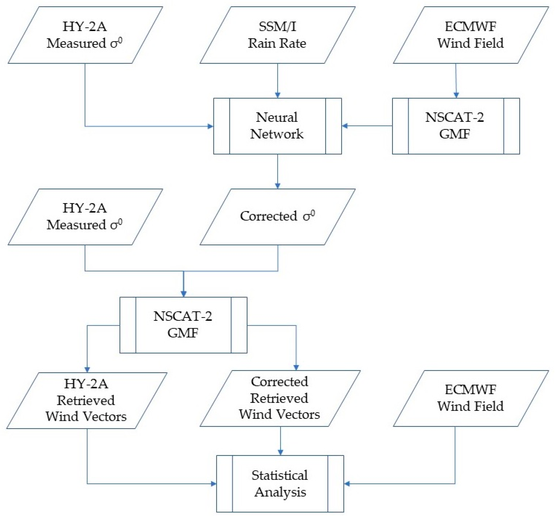
For comparison, we perform a statistical analysis on the accuracy of the backscatter measurements of the HY-2A scatterometer in the case of rain and no rain. In addition, the impact of rain on the backscatter coefficients of the HY-2A scatterometer is studied. The reference standards used are the predicted model backscatter coefficients calculated with the matched ECMWF winds through the NSCAT-2 model. The precision of the HY-2A backscatter coefficient under different rainfall conditions is estimated for different polarizations. The HY-2A scatterometer rainfall effect correction and verification process is shown in Figure 2. In modeling stage, the SSM/I rain rate data and the HY-2A measured σ0 data are the inputs of the neural network, while the ECMWF wind field data are used to calculate the model σ0 though the NSCAT-2 GMF, which is taken as the output of the neural network. The rainfall effect correction neural network model can be obtained through a training procedure. The corrected σ0 and the HY-2A measured σ0 are used to retrieve wind vectors respectively to validate the performance of the neural network for rainfall effect correction.

3.1. Analysis of Backscatter Coefficient without Rain

Figure 3a,b show the scatter plots of the HY-2A measurement σ0 and the ECMWF model σ0 data pairs under the condition of no rain. It can be observed that under either HH polarization or VV polarization, all the matched data points conform to obvious linear distribution characteristics. Due to the property of the measurement noise of the scatterometer and the influence of other random factors, such as satellite attitude variations, the precision of the backscatter coefficients measured by the scatterometer varies with different wind speeds, with a higher error under low wind speed conditions. That is, the scatter plots of the HY-2A measured σ0 and the ECMWF model σ0 at low wind speeds are more discrete. To further verify the error between the HY-2A measurement σ0 and the ECMWF model σ0, we divide the data samples into different wind speed intervals, with an interval length of 1 m/s, and the error statistics are calculated for the HY-2A measurement σ0 and the ECMWF model σ0 for each ECMWF wind speed interval. Table 2 presents the statistical results of the bias error between the measurement σ0 and the model σ0 (the measurement σ0 minus the model σ0) of each wind speed interval under the condition of no rain for different polarizations. In general, the average absolute error between the measurement σ0 of the HY-2A scatterometer and the ECMWF model σ0 is less than 1 dB. Therefore, the error of the measured σ0 by the HY-2A scatterometer is not too high under the condition of no rain.

3.2. Analysis of the Backscatter Coefficient under Rainy Conditions

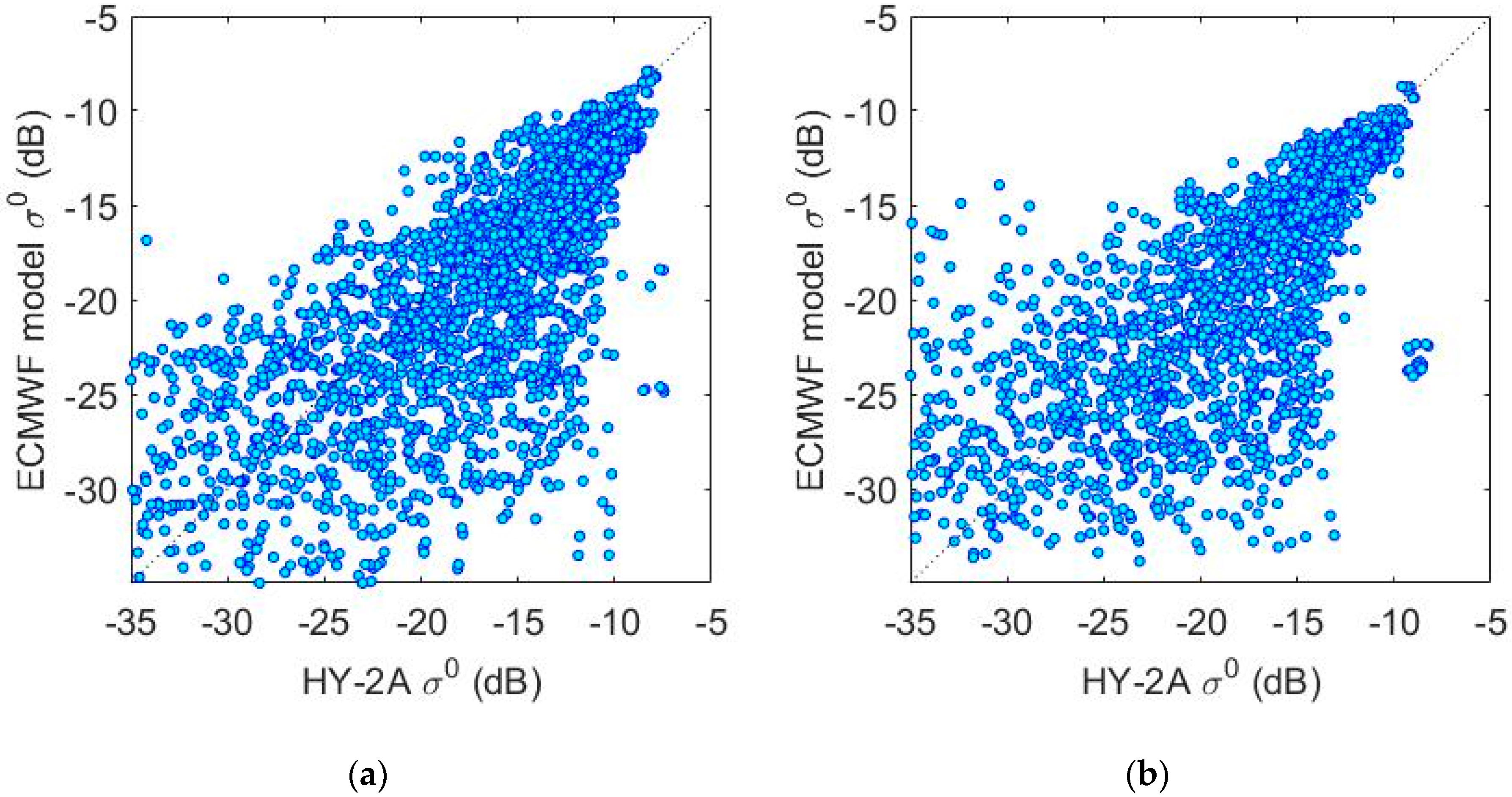
Figure 4a,b give the scatter plots of the HY-2A measurement σ0 and the ECMWF model σ0 under rainy conditions, Figure 4a for HH polarization, and Figure 4b for VV polarization. Compared with the matched data under the condition of no rain, the scatter plots of the HY-2A measurement σ0 and the ECMWF model σ0 under the condition of rain show obvious systematic deviation and are much more dispersed, indicating that the backscatter coefficients measured by the HY-2A scatterometer are strongly affected by rain under both HH and VV polarization. The sizes of raindrops depend on different rain rates, and different sizes of raindrops have different effects on the wind measurement of scatterometers. For each polarization, the matched data samples of the HY-2A measurement σ0 and the ECMWF model σ0 are divided into different bins by rain rate with an interval of 1 mm·h−1, and the error statistics are calculated for each bin. The results are capable of showing the impact of rain on the precision of the backscatter coefficients measured by the HY-2A scatterometer.
Table 3 shows the statistical results of the error between the HY-2A measurement σ0 and the ECMWF model σ0 under rainy conditions. The effect of rain on the backscatter coefficients measured by the HY-2A scatterometer rises with the increase of rain rate, and the increase of the wind speed will also add to the error of the backscatter coefficients measured by scatterometer. Table 3 lists the statistical results of the mean bias errors between the scatterometer measured σ0 and the model predicted σ0 within the rain rate range of 1–20 mm·h−1. The range of ECMWF wind speeds used to compute the bias and standard deviation errors in Table 3 is 1 to 24 m/s. The mean bias errors between the HY-2A measurement σ0 and the ECMWF model σ0 are calculated in decibel units. The bias errors under HH polarization and VV polarization caused by rain are both positive, indicating that the measured σ0 is greater than the model predicted σ0. Moreover, the mean bias errors increase with the increasing rain rate, indicating that the increase in rain rate causes the measured backscatter coefficients to be overestimated, and the extent of the overestimation in the backscatter coefficients increases with the increasing rain rate. From the statistical results of the standard deviation under HH polarization and VV polarization, it can be seen that, due to the influence of rain, there is increased uncertainty in the backscatter coefficients measured by the HY-2A scatterometer, which is quite different from the backscatter coefficients of the ECMWF model under the condition of no rain, and the same trend is reflected in the scatter plots.

3.3. Rainfall Effect Neural Network Correction Model

According to the analysis in Section 3.2, rain strongly affects the backscatter coefficients measured by the scatterometer. It is clear that the impact of rain on σ0 measured by the HY-2A scatterometer is a nonlinear physical process with great uncertainty. The BP (back propagation) neural network is a type of machine learning model that has a strong nonlinear fitting ability and is suitable for dealing with complex function modeling [28]. The BP neural network is composed of multilayer neurons. In the process of training the BP neural network, the signal is transmitted forward, and the error is propagated backward. In the process of forward transmission, the signal is used as the input for the first layer; then, it is processed by multiple hidden layers until it reaches the output layer. In the process of signal transmission, each neuron is given a weight and threshold, and the state of each neuron affects the next layer. The state of the output layer determines whether the neural network training is terminated or not. If the expected output is not obtained, the error propagates backward. According to the prediction error, the network adjusts the weights and thresholds of the neurons until the expected output is obtained or the number of training steps reaches the maximum; then, the training process ends.
As shown in Section 3.1, the ECMWF reanalysis wind is a reliable model-generated data product with high accuracy, and its accuracy is rarely affected by weather conditions such as rain. Because the amount of matched data between the buoy data and the HY-2A data is too small, the ECMWF reanalysis wind data are taken as the reference standard, and the effect of rain on σ0 measured by the scatterometer is corrected by artificial neural network fitting. The temporal coverage of the data we used to establish the correct model is from January 1 to June 31, 2013. In the process of BP neural network modeling, the quality and distribution of the data will affect the training process and prediction results. Generally, the distribution of sample points has a great influence on the training effect of the neural network. The distribution of sample points in the matched dataset is uneven. One of the outstanding characteristics is that there are fewer sample points in the high rainfall range. Therefore, if the input data sample for each iteration is just randomly selected from the original matched dataset, then the neural network will over-fit in the interval with more data samples while it will under-fit in the interval with fewer data samples. To avoid this effect, we present a balanced sampling strategy. In this study, the experimental data are classified by polarization, backscatter coefficient, and rain rate. The classification intervals of the backscatter coefficient and rain rate are 0.1 dB and 1 mm·h−1, respectively, and the ranges of the backscatter coefficient and rain rate are −45~−5 dB and 1~20 mm·h−1, respectively. To ensure the uniformity of the data point distribution, 100 data points are randomly extracted from each classification interval to comprise the modeling dataset. When the number of data points in one classification interval is less than 100, all the data points within that bin are selected and the missing data points are randomly selected from all the data points to make up to 100. Finally, we obtained 78,233 pairs of matched data for HH polarization and 72,497 pairs for VV polarization. Therefore, although there are less data under the condition of high rainfall, the same number of samples is still involved in the training. This strategy ensures that the neural network model can stably converge even when there are few data samples in certain classification interval. At the same time, in order to ensure the training effect, mean squared error (MSE) is used as the cost function, which evaluates the mean square of the difference between the predicted value and the measured value at the output of the neural network. The smaller the MSE, the better the training effect of the neural network. Only when the absolute difference between the MSEs of two adjacent iterations is less than a given threshold value (set to 0.00004 in this paper), the training ends.
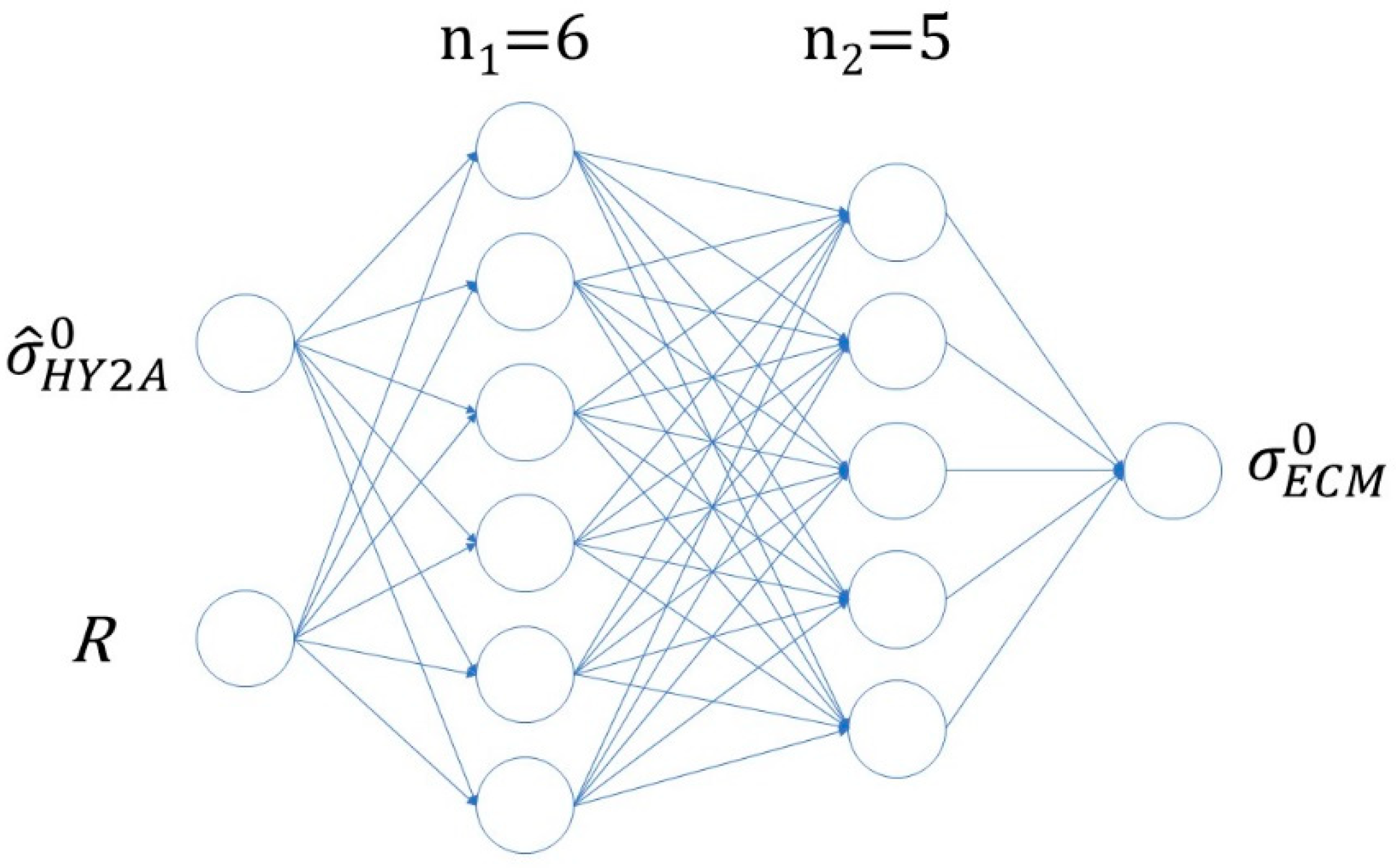
The topological structure of the BP neural network for correcting the rain effect of the measured backscatter coefficients is shown in Figure 5; this network has four layers, one input layer, two hidden layers, and one output layer. The number of nodes in each layer is 2, 6, 5, and 1. The inputs of the network include rain rate, which is represented as R, and the HY-2A measured backscattering coefficient denoted as σ ^ H Y 2 A 0 , and the output end is the ECMWF model backscattering coefficient shown as σ E C M 0 in Figure 4. Before training, both the inputs and output of the neural network are normalized, making all values fall in the interval [−1, 1]. The normalization equation is as follows:
y = ( y m a x y m i n ) ( x x m i n ) / ( x m a x x m i n ) + y m i n ,
where x is the value of input, y is normalized value of x, ymax is the maximum value of y, let it equal 1, ymin is the minimum value of y, let it equal −1, the xmax and xmin are, respectively, the maximum and minimum values of input data.
The first hidden layer has weights coming from the input. Each subsequent layer has a weight coming from the previous layer, all layers have biases, and the last layer is the network output. Two neural networks were established to correct the effect of rain on the σ0 measurement, one for HH polarization and the other for VV polarization.
The activation function is an important part of the neural network. If the activation function is not used, the input of each layer of the network is the linear output of the previous layer, so regardless of the number of layers in the neural network, the final output is a linear combination of the input, which is equivalent to the effect of the neural network without a hidden layer. This situation is the most primitive perception. Because of the above reasons, it is necessary to introduce a nonlinear function as the activation function so that the deep neural network is meaningful, and the output is no longer a linear combination of the input and can approximate any function.
In the rain effect correction neural networks, we employed sigmoid, identity and tanh as the activation functions in the different layers. The activation function of the first hidden layer is the sigmoid function, also known as the logistic function. For any input, its output range is (0, 1). The formula is as follows:
s i g m i o d ( z ) = 1 1 + e z ,
In the second hidden layer, the identity function is adopted as the activation function. In the identity activation function, the input of the node is equal to the output. It is perfect for tasks where the underlying behavior is linear. The identity activation function is as follows:
i d e n t i t y ( z ) = z ,
The activation function of the output layer is the tanh function. Tanh is completely differentiable and antisymmetric. It is a function with a center of symmetry at the origin. Tanh can transform the input into a suitable output range. Specifically, for any input, tanh will produce a value between −1 and 1. Compared with other transition function such as sigmoid, it is more sensitive and easier to converge when the data difference is obvious. Because of the advantages mentioned above, it is widely used in classification tasks. The tanh function is shown in formula (8):
tanh ( z ) = 2 1 + e 2 z 1 ,
The main parameters of the neural network training algorithm include the learning rate, epochs, and goal. The learning rate is the parameter that controls the size of the weight and bias changes in the learning of the training algorithm. In the rain effect correction model, the learning rate, the value of epochs, and the value of the goal are set to 0.1, 600, and 0.00004, respectively. The training will stop once the number of iterations exceeds the epoch value. When the neural network is trained by the minimum error, this value represents the maximum number of iterations. The goal of the training algorithm is usually defined as the minimum mean square error of the epoch, which is the sum of squared differences between the network targets and actual outputs divided by the number of training samples. In this study, these three parameters were empirically determined based on the performance of the neural network.

3.4. Wind Vector Retrieval Algorithm

To examine the performance of the neural network model in rain effect correction, a wind retrieval experiment will be conducted with the validation dataset. Since the model function relating σ0 with environmental variables and radar parameters is nonlinear, to find the optimal solution of wind vector inversion, a scatterometer wind field retrieval algorithm is introduced in [29]. The purpose of the wind vector retrieval algorithm is to determine the possible vector winds when the measured values of σ0 and σ0 calculated from the GMF are the most consistent and obtain wind speed and wind direction information. Although the wind vector retrieval algorithm plays a very important role in the process of scatterometer data processing, it is a numerical process, not an analytical one. Only when σ0 is noise-free, the GMF is accurately known, and σ0 is the only solution for the sea surface wind vector and radar parameter function can the inverse wind vector be completely resolved from more than three σ0 measurements. Sea surface wind vector retrieval is a “prior” problem; due to the influence of noise, the functional form of the statistical distribution is difficult to predict. To solve this a priori estimation problem, the maximum likelihood estimation (MLE) method is usually used as the wind vector retrieval algorithm of the microwave scatterometer ground processing flow [30]. In the process of wind retrieval, the wind vector solutions are determined by looking for the wind vectors that make the residual between the measured σ0 and the GMF predicted σ0 reach the minimum values. The objective function of the MLE method is as follows:
J MLE ( w , Φ ) = i = 1 N [ ( z k M ( w , Φ ) ) 2 Δ k + ln Δ k ] ,
where JMLE is the maximum likelihood value, which is a function of wind speed w and wind direction Φ; N is the number of σ0 measurements associated with different polarizations, azimuth angles and incidence angles in a wind vector cell; zk is the corresponding i-th measured value of σ0; M is the σ0 predicted by the GMF; w is wind speed; Φ is wind direction; and Δk represents the σ0 measurement variance caused by instrument noise.
The process of finding the inversion wind vector that makes the objective function reach a maximum value is highly nonlinear, so multiple wind vectors are usually obtained after the MLE optimization; they constitute a set of potential wind vector solutions for each wind vector cell. One of the solutions needs to be selected as the unique one. The process of determining the true solution from the set of potential solutions is called ambiguity removal. In this study, we use the ECMWF wind field as the reference and select the wind vector solution that has the minimum direction difference against the ECMWF wind as the true solution.

4. Result

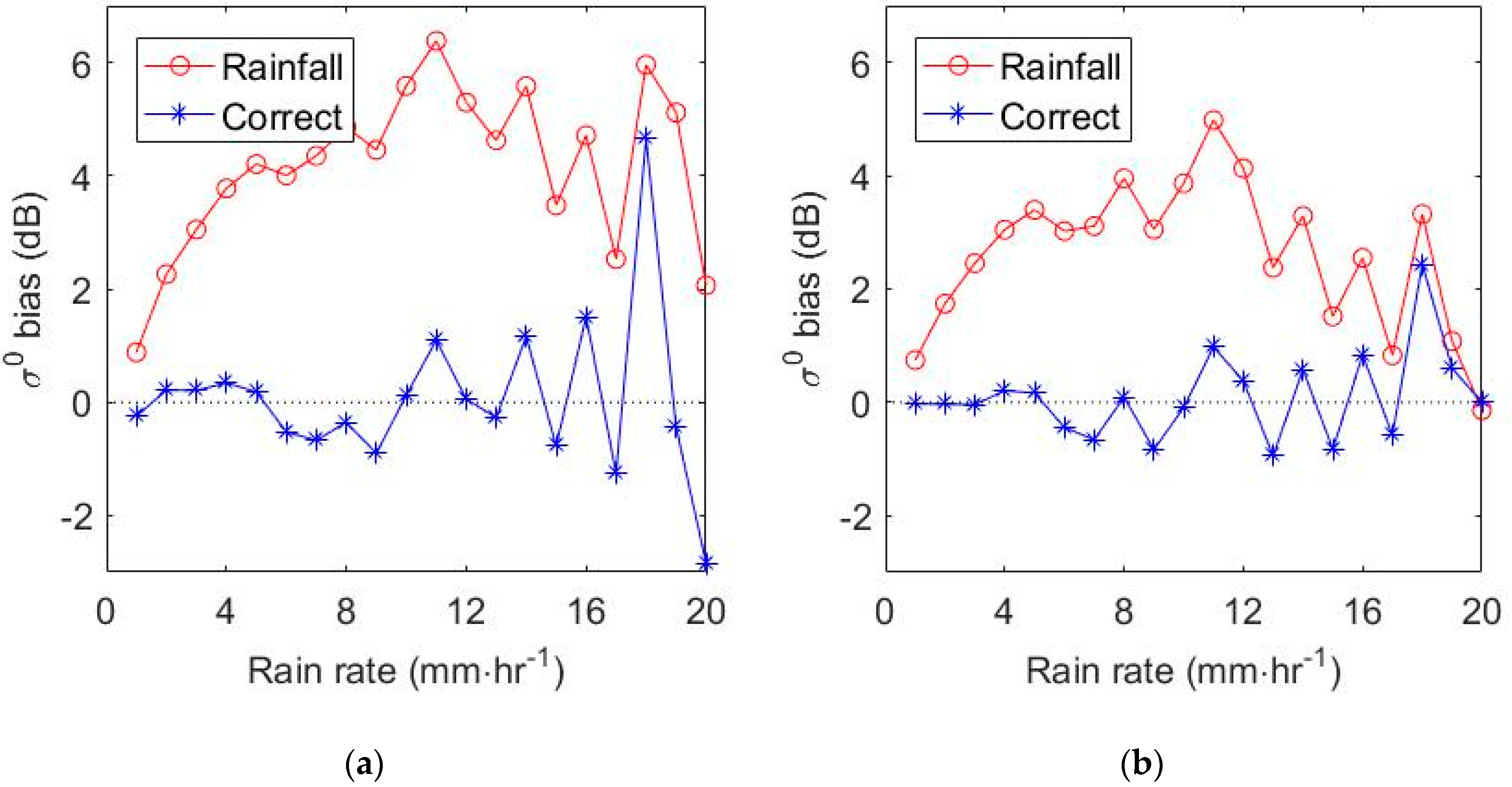
To generate the rainfall effect correction BP neural network, five-sixths of the HY-2A data and the corresponding ECMWF data are used as neural network modeling data, and the remaining one-sixth of the data are used for the model validation. The remaining validation data are used to verify the effectiveness of the neural network model in the correction of the rain-contaminated backscatter coefficients measured by the HY-2A scatterometer. There are 139,629 data pairs for VV polarization data and 150,720 data pairs for HH polarization that are used in verification. For comparison, the mean deviations (bias error) between the HY-2A measured σ0 and the ECMWF model σ0 and between the neural network predicted σ0 and the ECMWF model σ0 are computed for each classification interval of rain rate. The statistical results are shown in Figure 6. Figure 6a,b display the variation curves of the bias errors of σ0 versus the rain rate for HH polarization and VV polarization, respectively. In these two figures, the red circle in the figures denotes the mean deviation between the HY-2A measured σ0 and the ECMWF model σ0 (HY-2A measured σ0 minus ECMWF model σ0), and the blue asterisk denotes the mean deviation between neural network predicted σ0 and the ECMWF model σ0 (neural network predicted σ0 minus ECMWF model σ0). There is a clear trend in the figures, the mean deviation of the HY-2A measured σ0 minus the ECMWF model σ0 is positive. The mean deviation values for HH polarization and VV polarization show the same trend, indicating that the backscatter coefficients measured by the scatterometer are easily overestimated under both polarizations in the case of rain. In Figure 6a,b, the mean deviation value of the neural network predicted σ0 minus the ECMWF model σ0 shows that most of the mean deviation values fluctuate around the zero line without obvious systematic bias. When the rain rate is less than 16 mm·h−1, the absolute mean deviations are less than 2 dB, demonstrating that the difference between the neural network predicted σ0 and the ECMWF model σ0 is small.
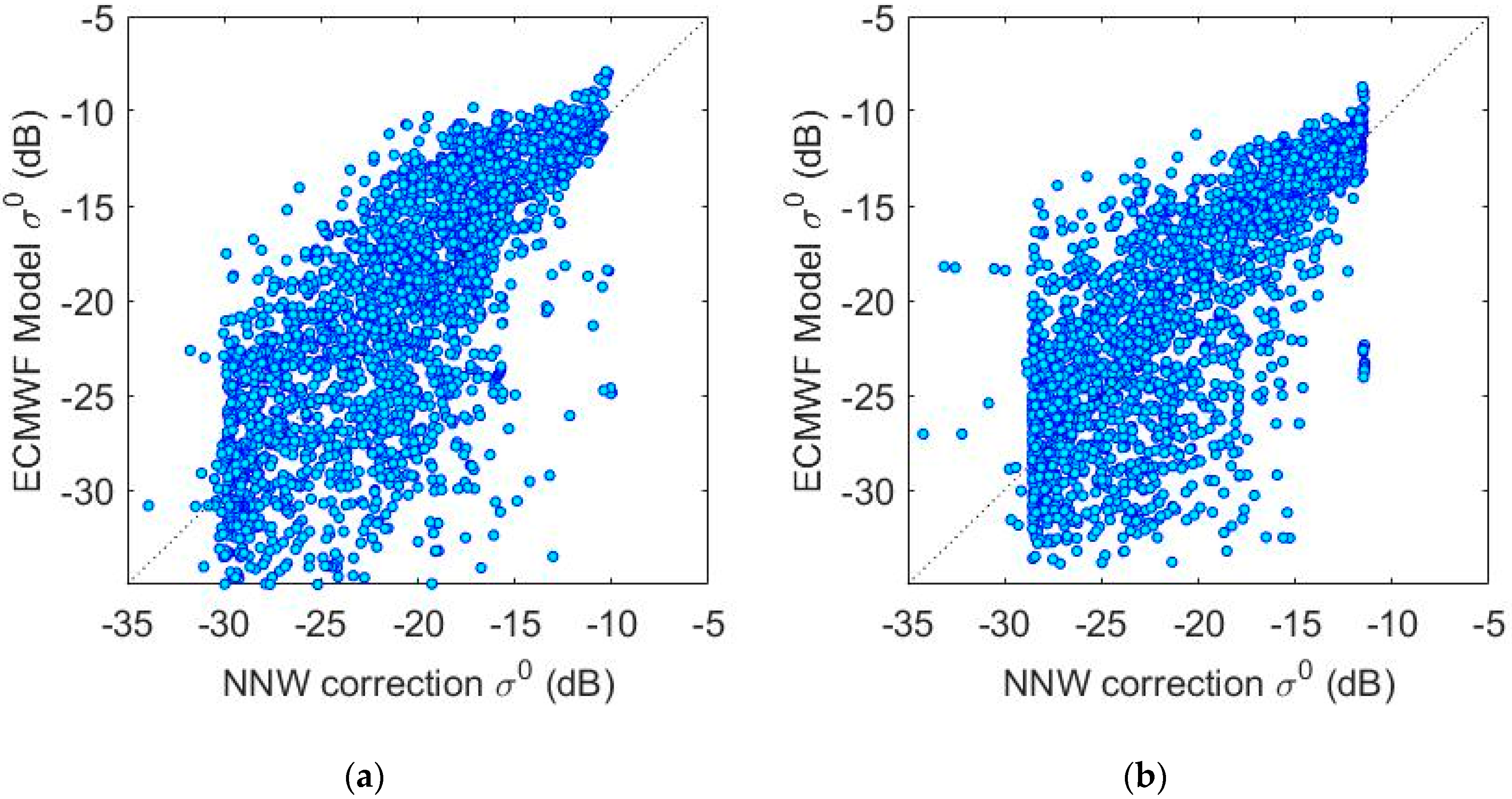
Figure 7a,b display the scatter plots of the neural network predicted σ0 and the ECMWF model σ0 under rain conditions for HH polarization and VV polarization, respectively. Compared with those of the HY-2A measured σ0 data and the ECMWF model σ0 in Figure 4a,b, the scatter plots of the neural network predicted σ0 and the ECMWF model σ0 are much more linear and concentrated.
Table 4 lists the statistical results of the mean bias error between the neural network predicted σ0 and the ECMWF model σ0 to show the correction effectiveness of the rain contaminated σ0 by the neural network model. In Table 4, the mean bias error and standard deviation of the neural network predicted σ0 minus the ECMWF model σ0 are calculated within each classification interval of rain rate over the range of 1–20 mm·h−1 for both polarizations. From the statistical results, it can be seen that the absolute value of the mean bias error between the neural network predicted σ0 and the ECMWF model σ0 is basically less than 1 dB. The standard deviations between the neural network predicted σ0 and the ECMWF model σ0 are not very different from those between the HY-2A measured σ0 and the ECMWF model σ0, which is consistent with the distribution characteristics of the scatter plots. As shown in Table 4, the neural network model significantly improved the accuracy of the backscatter coefficients contaminated by rain, in which the overestimation of the backscatter coefficients caused by rain was corrected to a large extent.
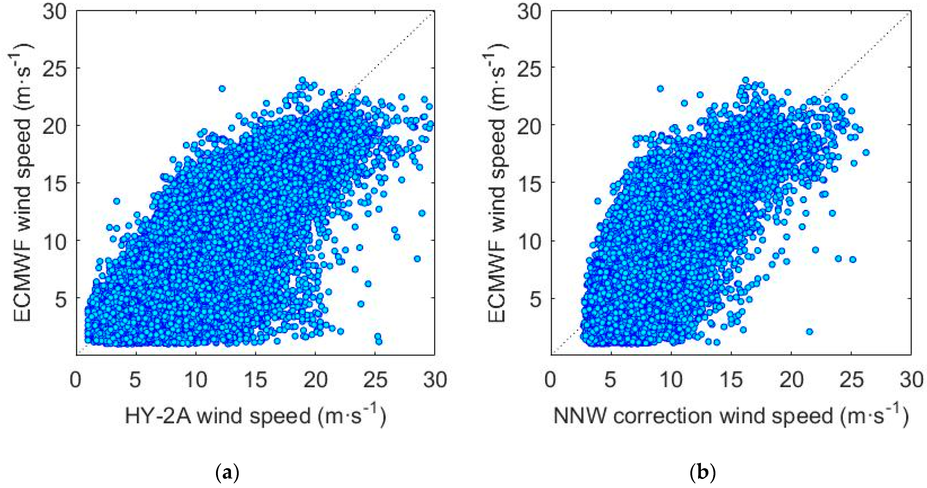
To further validate the effectiveness of the neural network model, wind retrieval experiments are conducted using the backscatter coefficients measured by the HY-2A scatterometer without rain effect correction and the backscatter coefficients corrected by the neural network. The retrieved wind vector data of the HY-2A measured σ0 and the retrieved wind vector data of the neural network corrected σ0 are obtained. Figure 8a shows the scatter plots of the HY-2A-retrieved wind speeds without rain effect correction and the matched ECMWF wind speeds. The horizontal coordinate is the HY-2A retrieved wind speed without rain effect correction, while the vertical coordinate is the ECMWF wind speed. The scatter plot reflects that rain causes the retrieved wind speeds from the HY-2A scatterometer to be overestimated when the measured backscatter coefficients are not corrected, which is consistent with the characteristics of the backscatter coefficients. Figure 8b shows the scatter plot of the retrieved wind speeds from the neural network predicted σ0 and the corresponding ECMWF wind speeds. In this figure, the horizontal coordinate is the retrieved wind speed from the neural network predicted σ0. Compared with Figure 8a, it is clear that the systematic deviation of the retrieved wind speeds caused by rain has been effectively corrected, indicating that the neural network model can improve the accuracy of the retrieved wind speeds under rainy conditions.
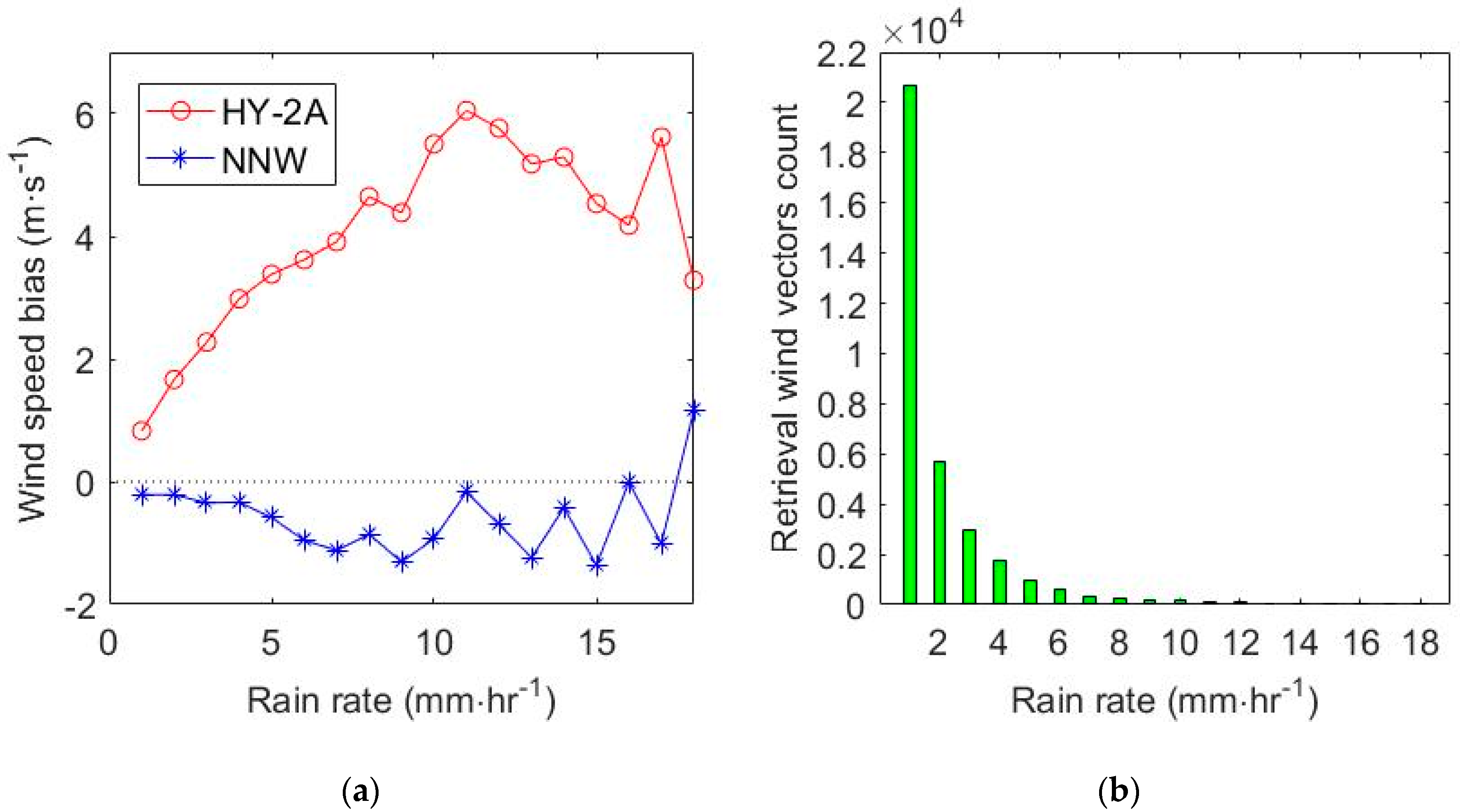
Figure 9a shows the statistical results of the wind speed biases between the retrieved wind speeds of the HY-2A scatterometer affected by rain and the ECMWF model wind speeds and those between the retrieved wind speeds from the neural network corrected σ0 and the ECMWF model wind speeds. The wind speed bias is calculated for each classification interval of rain rate. The classification interval of rain rate is 1 mm·h−1, and the range of rain rate is 1–18 mm·h−1. The red circle in Figure 9a represents the mean bias error between the HY-2A retrieved wind speeds and the ECMWF wind speed (HY-2A minus ECMWF), and the blue asterisk represents the mean bias error between the retrieved wind speeds from the neural network corrected σ0 and the ECMWF wind speeds (NNW minus ECMWF). The error first increases with the increasing rain rate and then decreases with the increasing rain rate. Figure 9a indicates that the impact degree of rain on the retrieved wind speeds first increases with the increasing rain rate and then decreases with the increasing rain rate, which is consistent with the effect trend of rain rate on the backscatter coefficients. Figure 9b gives a statistical histogram of the number of retrieved wind speeds in each rain rate interval. Figure 9b clearly shows that the number of retrieved wind speed samples in each interval declines sharply with the increase in rain rate. When the rain rate is high, there are fewer matched data samples used for training the neural network and verification, so the curve of the wind speed bias tends to fluctuate. From Figure 8, we can conclude that the impact of rain on the wind retrieval of the scatterometer causes the wind speeds to be overestimated.
We calculated the deviations between the HY-2A retrieved wind speeds affected by rain and the ECMWF wind speeds and the deviations between the retrieved wind speeds from the neural network corrected σ0 and the ECMWF wind speeds for each rain rate interval of 1 mm·h−1 over the range of 1–20 mm·h−1. The statistical results are shown in Table 5. Table 5 shows that under the impact of rain, the error of wind speed measured by scatterometer rises with an increase in rain rate, and the absolute value of the bias error of wind speed retrieved from the neural network corrected σ0 is less than 2 m/s, which is consistent with the signature reflected in Figure 8a, indicating that the neural network model has a significant effect on correcting the systematic error in wind speed retrieved by the HY-2A scatterometer under rainy conditions.

5. Discussion

In Section 3, we compute and analyze the bias and standard deviation values between the neural network corrected σ0 and the HY-2A measured σ0 for different polarizations. The results indicate that the impact of the rain tends to increase the measured σ0 value. In error statistics, the error of the HY-2A σ0 caused by rain first increases and then decreases with the increasing rain rate. It should be noted that when the rain rate is greater than 11 mm·h−1, the number of observed data points is less, and the mean deviation fluctuates irregularly. When the rain rate is less than 11 mm·h−1, the mean deviation increases regularly with increasing rain rate, indicating that under such rain conditions, the disturbance of sea capillary waves caused by rain and the body backscattering of raindrops in the atmosphere are dominant. When the rain rate is greater than 16 mm·h−1, the bias error between the neural network predicted σ0 and the ECMWF model σ0 fluctuates strongly due to the fewer matched σ0 data pairs used for training and testing. Due to insufficient knowledge of the mechanism of the rain effect on the backscatter coefficients measured by the scatterometer and the impact of other environmental factors, the scatter plots of the neural network predicted σ0 and the ECMWF model σ0 show a slight dispersion, but the neural network model has a certain effect on correcting the systematic errors in the measured σ0 caused by rain. Compared with the case without correction, the neural network predicted σ0 is much closer to the ECMWF model σ0, illustrating that most deviations of the backscatter coefficients contaminated by rain have been effectively removed.
The error analysis of the retrieved winds by the neural network predicted σ0 and the HY-2A measured σ0 can further verify the correction effect of the neural network on the impact of rain in the scatterometer measurements. Rain causes overestimates in the backscatter coefficients measured by the scatterometer, so this effect should be reflected in the retrieved wind speeds, which are also overestimated. In contrast, the retrieved wind directions are less affected by rain; thus, we mainly examine the impact of rain on the retrieved wind speeds. The mean bias between the retrieved wind speeds with the neural network corrected σ0 and the ECMWF wind speeds is close to the zero with a small negative deviation. The absolute value of the mean bias is much smaller than that of the retrieved wind speeds without rain effect correction. Hence, the neural network can reduce the rain effect on the scatterometer to a large extent, which leads to an improvement of the wind speed retrieval under rainy conditions.
In this study, we applied the SSM/I rain rate data as input for the neural network rain effect correction modeling and validation. The main reason for choosing other satellite radiometer data as input is that the radiometer onboard the HY-2A satellite has no 85 or 89 GHz frequency channel, which are considered to be the necessary frequency bands for accurate rain rate estimation. Thus, the HY-2A radiometer currently does not provide the rain rate parameter. However, it should be noted that there are some limitations in using the SSM/I radiometer data as input. First, the presented approach depends on external data, which reduces its practical value. Second, only parts of the HY-2A scatterometer data are collocated with the SSM/I data due to the different temporal and spatial coverages of these two satellites. The main purpose of this study is to explore the feasibility of the neural network model to correct the rain effect and lay a technical foundation for the wind field inversion of the subsequent satellite scatterometers. The follow-up HY-2 satellites will have the capability of rain rate observation. In that case, we can directly use the rain rate data measured by the HY-2 radiometer as the model input to correct the rain effect.
In summary, the influence of rainfall on the retrieved wind speeds of the HY-2A scatterometer can be reduced by the method of neural network correction. The mean bias errors of wind speeds decreased from 1.48m/s to 0.28m/s. Compared with the results of other researchers, the effect of this method is nearly in the same order of magnitude. Due to the complexity and insufficient knowledge of the physical mechanism of the rain effect, there is still room for improvement of the correction model to completely remove rain contamination.

6. Conclusions

The data used in this study include the backscatter coefficients measured by the HY-2A scatterometer, the ECMWF reanalysis wind field data, the SSM/I radiometer-measured rain rate data, and the TAO buoy wind data. We verified the accuracy of the ECMWF reanalysis wind field data with some collocated TAO wind data before modeling. The deviations of the HY-2A measured σ0 from the ECMWF model σ0 are calculated and analyzed under rainy and no-rain conditions. A neural network model is established based on the matched data pairs of the HY-2A measured σ0 and the ECMWF model σ0 under rainy conditions. The following three conclusions are drawn through experiments.
First, by comparing the mean bias error and standard deviation of the HY-2A measured σ0 and the ECMWF model σ0 under the conditions of rain and no rain, we found that the mean deviation of the matched data is increased under the condition of rain, which indicates that rain interferes with the backscattering coefficients measured by the HY−2A scatterometer, resulting in a systematic deviation in the HY-2A measured σ0. In rainy conditions, the mean deviation between the HY-2A measured σ0 and the ECMWF model σ0 is positive and increases with the increasing rain rate. In the rain rate range of 1–20 mm·h−1, body backscattering and the disturbance of sea capillary waves caused by raindrops enhance the received signal energy of the scatterometer, which leads to the overestimation of backscatter coefficients measured by the scatterometer under rainy conditions. Comparatively, the experimental results indicated that the inaccuracy of the backscatter coefficients measured by the HY-2A scatterometer under the condition of rain can be effectively improved by the neural network model.
Second, from the comparison between the HY-2A retrieved wind speed and the ECMWF wind speed and that between the retrieved wind speed from the neural network corrected σ0 and the ECMWF wind speed under the condition of rain, it can be concluded that the neural network model effectively corrects the systematic deviation of the wind speeds caused by rain and improves the accuracy of the wind speed retrieval. The results show that the neural network model can be used to correct the systematic deviation of wind speed caused by rain.
Finally, due to the limitations of the present data set and the uneven data distribution, the established neural network in this study probably is only reliable and applicable under specific conditions. Since there are not enough data with rain rates greater than 16 mm·h−1, the accuracy of the neural network model under such conditions needs further verification. Due to the mechanism of scatterometer wind measurement, different wind speed conditions also affect the accuracy of wind field retrieval. When the sea surface wind speed is too low, such as less than 4 m·s−1, the instrument and geophysical noise have a strong influence on the wind retrieval accuracy. Thus, when the wind speed is too low, the effect of the neural network model is also limited. Therefore, the conclusion of the model established in this paper is only applicable to data in a certain wind speed range, and more data will be used to verify and improve the model in future work.

Author Contributions

Conceptualization, investigation, writing-review and editing, project administration and funding acquisition, X.X.; Data curation, methodology, software, writing-original draft, J.W.; Formal analysis, validation, supervision, M.L. All authors have read and agreed to the published version of the manuscript.

Funding

This work was funded in part by the National Natural Science Foundation of China under grant 41876204 and grant 41476152, and in part by the National Key Research and Development Project of China under grant 2016YFC1401001, and in part by Special Fund Project for Marine Economic Development of Guangdong Province under grant GDNRC [2020]013.

Acknowledgments

The authors would like to thank the European Centre for Medium-Range Weather Forecasts (ECMWF), the National Data Buoy Center (NDBC), and the Remote Sensing Systems (RSS) for providing the reanalysis wind field data, the buoy data, and the SSM/I radiometer rain rate data, respectively.

Conflicts of Interest

The authors declare no conflicts of interest.

References

  1. Wright, J. Backscattering from capillary waves with application to sea clutter. IEEE Trans. Antennas Propag. 1966, 14, 749–754. [Google Scholar] [CrossRef]
  2. Portabella, M. Wind Field Retrieval from Satellite Radar Systems. Ph.D. Thesis, University of Barcelona, Barcelona, Spain, 2002. [Google Scholar]
  3. Zhong, J.; Huang, S.X.; Zhang, L. Research on the development of surface wind retrieval from microwave scatterometer. J. Meteorol. Sci. 2010, 30, 137–142. [Google Scholar]
  4. Brown, R.A. On satellite scatterometer model functions. J. Geophys. Res. 2000, 105, 29195–29205. [Google Scholar] [CrossRef] [Green Version]
  5. Stoffelen, A.; Verspeek, J.; Vogelzang, J.; Verhoef, A. The CMOD7 geophysical model function for ASCAT and ERS wind retrievals. IEEE J. Sel. Top. Appl. Earth Obs. Remote Sens. 2017, 10, 2123–2134. [Google Scholar] [CrossRef]
  6. Chi, C.Y.; Li, F.K. A comparative study of several wind estimation algorithms for spaceborne scatterometers. IEEE Trans. Geosci. Remote Sens. 1988, 26, 115–121. [Google Scholar] [CrossRef]
  7. Freilich, M.H.; Dunbar, R.S. Derivation of satellite wind model functions using operational surface wind analyses—An altimeter example. J. Geophys. Res. 1993, 98, 14633–14649. [Google Scholar] [CrossRef]
  8. Schultz, H. A circular median filter approach for resolving directional ambiguities in wind fields retrieved from spaceborne scatterometer data. J. Geophys. Res. 1990, 95, 5291–5303. [Google Scholar] [CrossRef]
  9. Lin, M.S.; Zheng, S.Q.; Sun, Y. A study on a new dealias algorithm for retrieval of oceanic wind vectors field. J. Oceanogr. Taiwan Strait 1996, 15, 243–254. [Google Scholar]
  10. Wang, L.; Lu, H.C.; Pan, X.B.; Zhang, Y. Correction of asymmetric strengthening of QuikSCAT wind field and assimilation application in typhoon simulation. J. Trop. Meteor. 2009, 15, 78–82. [Google Scholar]
  11. Contreras, R.; Plant, W. Surface effect of rain on microwave backscatter from the ocean: Measurements and modeling. J. Geophys. Res. 2006, 111, 4105–4108. [Google Scholar] [CrossRef] [Green Version]
  12. Draper, D.; Long, D. Evaluating the effect of rain on SeaWinds scatterometer measurements. J. Geophys. Res. 2004, 109, 235–250. [Google Scholar] [CrossRef] [Green Version]
  13. Draper, D.W.; Long, D.G. Simultaneous wind and rain retrieval using SeaWinds data. IEEE Trans. Geosci. Remote Sens. 2004, 42, 1411–1423. [Google Scholar] [CrossRef]
  14. Yueh, S.H.; Stiles, B.W.; Liu, W.T.L. QuikSCAT wind retrievals for tropical cyclones. IEEE Trans. Geosci. Remote Sens. 2003, 41, 2616–2628. [Google Scholar] [CrossRef] [Green Version]
  15. Weissman, D.E.; Bourassa, M.A.; Tongue, J. Effects of rain rate and wind magnitude on SeaWinds scatterometer wind speed errors. J. Atmos. Ocean. Technol. 2002, 19, 738–746. [Google Scholar] [CrossRef]
  16. Nielsen, S.N.; Long, D.G. A wind and rain backscatter model derived from AMSR and SeaWinds data. IEEE Trans. Geosci. Remote Sens. 2009, 47, 1595–1606. [Google Scholar] [CrossRef]
  17. Allen, J.R.; Long, D.G. An analysis of SeaWinds-based rain retrieval in severe weather events. IEEE Trans. Geosci. Remote Sens. 2005, 43, 2870–2878. [Google Scholar] [CrossRef]
  18. Stiles, B.; Dunbar, R. A neural network technique for improving the accuracy of scatterometer winds in rainy conditions. IEEE Trans. Geosci. Remote Sens. 2010, 48, 3114–3122. [Google Scholar] [CrossRef]
  19. Gohil, B.S.; Sikhakolli, R.; Gangwar, R.K.; Kumar, A.S.K. Oceanic rain flagging using radar backscatter and noise measurements from oceansat-2 scatterometer. IEEE Trans. Geosci. Remote Sens. 2016, 54, 2050–2055. [Google Scholar] [CrossRef]
  20. Lin, W.; Portabella, M.; Stoffelen, A.; Turiel, A.; Verhoef, A. Rain identification in ASCAT winds using singularity analysis. IEEE Geosci. Remote Sens. Lett. 2014, 11, 1519–1523. [Google Scholar] [CrossRef] [Green Version]
  21. Owen, M.P.; Long, D.G. Simultaneous wind and rain estimation for QuikSCAT at ultra-high resolution. IEEE Trans. Geosci. Remote Sens. 2011, 49, 1865–1878. [Google Scholar] [CrossRef]
  22. Li, J.; Tjuatja, S.; Dong, X.; Zhu, D. Impact of rainfall on a Ku-band rotating fan-beam scatterometer. J. Remote Sens. 2013, 17, 98–106. [Google Scholar]
  23. Zou, J.H.; Xie, X.T.; Zhang, Y.; Lin, M.S. Wind Retrieval Processing for HY-2A Microwave Scatterometer. In Proceedings of the 2014 IEEE International Geoscience and Remote Sensing Symposium, Quebec City, QC, Canada, 13–18 July 2014. [Google Scholar]
  24. Thomas, B.; Kent, E.; Swail, V. Methods to homogenize wind speeds from ships and buoys. Int. J. Climatol. 2005, 25, 979–995. [Google Scholar] [CrossRef]
  25. Bozzano, R.; Siccardi, A.; Schiano, M.E.; Borghini, M.; Castellari, S. Comparison of ECMWF surface meteorology and buoy observations in the Ligurian Sea. Elsevier Oceanogr. 2004, 22, 87–91. [Google Scholar] [CrossRef] [Green Version]
  26. Freilich, M.H. SeaWinds Algorithm Theoretical Basis Document. Available online: http://podaac.jpl.nasa.gov/quikscat/qscat-doc/html (accessed on 18 March 2002).
  27. Wentz, F.J.; Smith, D.K. A model function for the ocean-normalized radar cross section at 14 GHz derived from NSCAT observations. J. Geophys. Res.: Ocean. 1999, 104, 11499–11514. [Google Scholar] [CrossRef]
  28. Skrzypek, J. Neural Network Simulation Environments; Springer: Los Angeles, CA, USA, 1994; pp. 120–130. [Google Scholar]
  29. Portabella, M.; Stoffelen, A. A probabilistic approach for SeaWinds data assimilation. QJR Meteorol. Soc. 2004, 130, 127–152. [Google Scholar] [CrossRef] [Green Version]
  30. Vries, J.; Stoffelen, A.; Beysens, J. Ambiguity Removal and Product Monitoring for SeaWinds. Available online: https://www.researchgate.net/publication/239784690_Ambiguity_Removal_and_Product_Monitoring_for_SeaWinds (accessed on 20 March 2020).
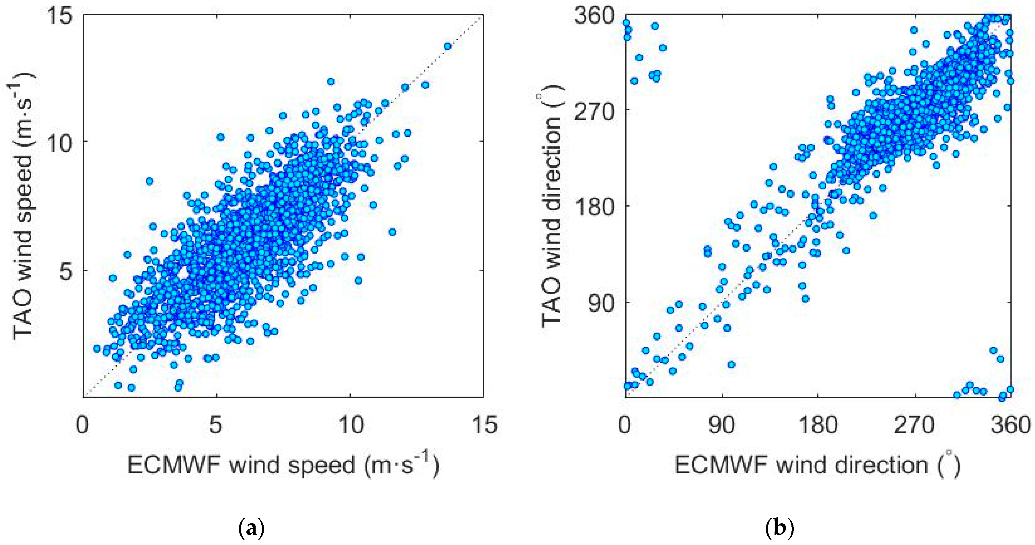
Figure 1. Scatter plots of TAO and ECMWF paired data. (a) Scatter plots of wind speed; (b) Scatter plots of wind direction. The dashed line in this figure is the diagonal line.
Remotesensing 12 01648 g001
Figure 2. Flow chart of the HY-2A scatterometer neural network rainfall effect correction.
Remotesensing 12 01648 g002
Figure 3. Scatter plot of measureσ0 and modelσ0 paired data without rainfall. (a) for HH polarization; (b) for VV polarization. The dashed line in this figure is the diagonal line.
Remotesensing 12 01648 g003
Figure 4. Scatter plot of measure σ0 and model σ0 paired data with rainfall. (a) for HH polarization; (b) for VV polarization. The dashed line in this figure is the diagonal line.
Remotesensing 12 01648 g004
Figure 5. Schematic diagram of BP neural network topology.
Remotesensing 12 01648 g005
Figure 6. Dependence of σ0 residual on the SSM/I rain rate. The red circle in the figure is the mean value of deviation of HY-2A measurement σ0 minus ECMWF model σ0, and the blue asterisk is the mean value of deviation of neural network correction σ0 minus ECMWF model σ0. (a) for HH polarization; (b) for VV polarization.
Remotesensing 12 01648 g006
Figure 7. Scatter plot of NNW correction σ0 and model σ0 paired data with rainfall. (a) for HH polarization; (b) for VV polarization. The dashed line in this figure is the diagonal line.
Remotesensing 12 01648 g007
Figure 8. Scatter plot of HY-2A wind speed and NNW wind speed with ECMWF wind speed. (a) for HH polarization; (b) for VV polarization. The dashed line in this figure is the diagonal line.
Remotesensing 12 01648 g008
Figure 9. Dependence of wind speed residual and number statistics on the SSM/I rain rate. (a) The result of error verification, the dashed line in the figure represents σ0 bias is 0; (b) The number of matched data samples.
Remotesensing 12 01648 g009
Table 1. ECMWF wind field data and TAO sea surface wind velocity data statistical analysis.
BiasStandard Deviation
Wind speed−0.00521.3467
Wind direction−1.685014.4374
Table 2. Dependence of σ0 residual (HY-2A-ECMWF) on the ECMWF wind speed statistical analysis.
ECMWF Wind Speed (m·s−1)HH-pol (dB)VV-pol (dB)
4−0.7971−0.5566
5−1.0560−0.7881
6−0.9248−0.7194
7−0.7961−0.5989
8−0.5841−0.4099
9−0.5713−0.3740
10−0.4625−0.3628
11−0.3737−0.3808
12−0.2744−0.3322
13−0.2369−0.2681
14−0.1091−0.1836
15−0.1398−0.0868
16−0.01610.0660
170.05400.1415
180.15060.1849
190.32700.3672
200.27860.3579
210.18000.3920
220.31080.2426
230.3420−0.0434
240.35950.1168
Table 3. HY-2A measure σ0 and ECMWF model σ0 statistical analysis.
Rain Rate (mm·h−1)Bias (dB)Standard Deviation (dB)
HH-polVV-polHH-polVV-pol
10.88100.74664.14243.7829
22.26171.74394.92334.2775
33.05092.45745.28224.7124
43.77653.04865.43444.8975
54.20573.39735.67494.8612
64.00593.02215.56874.6850
74.35073.11275.11134.5176
84.85473.95255.53165.1866
94.45413.05335.18934.2722
105.58663.86645.65835.2931
116.38034.98116.15905.6455
125.29454.12874.91964.8473
134.62432.37585.47994.3731
145.58023.28874.93694.3286
153.47541.51733.29062.9760
164.71152.54884.55844.1609
172.52860.83132.26792.1763
185.95943.32224.93913.9919
195.11641.07810.81020.8454
202.0640−0.13741.36600.9191
Table 4. NNWσ0 and ECMWF modelσ0 statistical analysis.
Rain Rate (mm·h−1)Bias (dB)Standard Deviation (dB)
HH-polVV-polHH-polVV-pol
1−0.2464−0.02493.98493.5596
20.2119−0.03434.80964.1298
30.2066−0.03645.17804.5098
40.34280.20715.30844.5923
50.18020.16685.60494.5560
6−0.5262−0.44235.49734.4841
7−0.6743−0.65984.97514.2717
8−0.35430.09225.42824.9399
9−0.9041−0.83385.02554.0298
100.1220−0.09325.61525.0522
111.09560.97916.06425.6303
120.05640.37884.92574.7773
13−0.2753−0.94575.29844.3006
141.16170.57744.85594.1675
15−0.7756−0.82732.97292.9511
161.50960.83454.90014.1017
17−1.2580−0.57852.71152.1361
184.65142.43706.56553.9099
19−0.43570.60170.68380.7682
20−2.8396−0.00211.49180.9214
Table 5. The errors of HY-2A wind speed and NNW wind speed with ECMWF wind speed.
Rain Rate (mm·h−1)Bias (m·s−1)Standard Deviation (m·s−1)Count
HY-2ANNWHY-2ANNW
10.8278−0.21082.52462.395120,706
21.6651−0.21392.95672.81285663
32.2736−0.34763.26043.03673000
42.9814−0.33403.52173.19101755
53.3827−0.58703.74993.3487942
63.6176−0.95614.01083.4617574
73.9107−1.11944.18053.4155342
84.6463−0.85564.37033.6356270
94.3848−1.30924.44433.5175201
105.5052−0.93155.19694.1480150
116.0519−0.16815.37934.2121125
125.7634−0.69554.66534.1094102
135.1812−1.23885.37734.366560
145.2926−0.42564.70883.973544
154.5338−1.36204.06213.298324
164.1803−0.00864.05624.433418
175.6187−1.01133.46572.436410
183.28401.15904.76426.47804