1. Introduction
The construction process of large-scale civil engineering development projects, such as quarry development projects, creates numerous soil-cutting and soil-banking slopes. If the cutting and banking slopes at a construction site are left unrestored for a long time, intense rainfall leads to soil erosion and subsequent damage to the surrounding river streams via deposition onto river beds. Problems such as collapsed soil slopes can arise depending on the treatment conditions associated with the cutting and banking slopes. In Korea, environmental impact assessments are conducted in accordance with the Environmental Impact Assessment Act to prevent problems that may arise from forest land development and quarry development projects. The environmental impact assessments for quarry development projects suggest that environmental pollution prevention measures, such as the installation of dustproof covers to reduce the occurrence of scattered dust due to the long-term stacking of waste stockpiles and the installation of waterproof covers to reduce soil leaks during the rainy season, should be implemented in the project sites. The impact of these projects on the environment should be minimized by continuous monitoring and rapid treatment of stacked waste stockpiles. Developers should be able to periodically maintain the treatment conditions of waste stockpiles by accurately and quickly computing its volume.
Traditional stockpile volume measurement methods include the truckload-and-bucket-count method and the eyeballing method. The truckload-and-bucket-count method is useful for computing a small stockpile volume; however, it takes a long time to compute a large-scale stockpile volume. Computing a volume using the eyeballing method is also plagued by significantly lower accuracy as computations are roughly performed based on the user’s estimated measurements. With advances in technology, global positioning system (GPS) or terrestrial laser scanning (TLS) can be used to compute the volumes more efficiently. TLS has been used to estimate the volume in various fields [
1]. The primary objective of TLS is to compute the distance from the lens to each object based on the range and time the light reflected by the object surface takes to reach the lens [
2].
TLS-based point cloud generation has applications in numerous fields (e.g., industry, forestry, and academic research) [
3,
4,
5,
6,
7]. Pitkänen et al. [
3] employed TLS in stem diameter measurements for a more accurate volume estimation, while Liu et al. [
4] measured leaf angle distribution affecting the flux of radiation, carbon, and water. Cultural heritage sites or buildings can be represented as point clouds for observation or monitoring purposes [
5,
8]. Xu et al. [
9] utilized TLS to monitor the annual surface elevation of glaciers and their accurate boundary measurements. Osada et al. [
10] proposed a method to minimize the Global Navigation Satellite System (GNSS) measurements in places such as city corridors where GNSS signals are weak. The TLS method has been intensively employed due to its ability to generate high-accuracy data with dense TLS-based three-dimensional (3-D) point clouds [
6,
11]. This method, however, is suboptimal (in terms of utility) due to its high cost and time consumption [
12]. There are numerous limitations with respect to monitoring waste stockpiles using TLS at project sites located in areas of danger, such as mountainous areas, where access is poor due to surrounding environmental features [
13]. The danger intensifies as people approach the waste mounds. Wastes create unpredictable landscapes that are difficult to walk on and may cause respiratory or skin problems depending on their type. Due to the limited access on foot, a ladder is used to reach the waste mound top and place ground control points (GCPs).
With the recent developments in computer vision technology, unmanned aerial vehicles (UAVs) have been widely used to complement the limitations of TLS [
14,
15] in various fields such as weed control [
16] (Pérez-Ortiz et al., 2016), agriculture mapping [
17], forest phenology [
18], forest structure [
19], and disaster prevention [
20,
21]. There has been a recent surge of research on the generation of point clouds using photogrammetry based on UAVs (also known as “drones”) to achieve location accuracy [
22,
23,
24]. The UAV-based orthoimages are employed to generate point clouds based on the scale-invariant feature transform and structure from motion (SfM) algorithms. Point clouds are also used to construct digital elevation models (DEMs), digital surface models (DSMs), and digital terrain models (DTMs).
The quality of a point cloud depends on various flight parameters (e.g., flight altitude and image overlap, GCPs), which have been the focus of numerous studies [
23,
25,
26,
27]. Agüera-Vega et al. [
23] evaluated the accuracy of images constructed using UAVs according to the number of GCPs. Mesas-Carrascosa et al. [
26] extracted the most accurate orthomosaic images in a wheat field based on different flight altitudes, flight modes (stop and cruise mode), and GCP settings. Furthermore, Mesas-Carrascosa et al. [
25] conducted an aerial survey of an archaeological area using the flight altitude, overlap setting, and number of GCPs as flight parameters. Dandois et al. [
27] compared the canopy height obtained in a deciduous forest by setting the altitude and the overlap against field data and airborne LiDAR data.
UAV technology has the advantages of accessibility and efficient site maintenance by periodic monitoring and thus is cheaper and less time-consuming than TLS; however, TLS can generate denser and more accurate point clouds [
11,
14,
28]. Relatively limited research has been conducted on point cloud generation or volume computation using TLS and UAV technologies in an integrated manner. Müller et al. [
29] mapped a study area using both TLS and UAV methods for eruption site monitoring, as both approaches can be selected depending on the technological characteristics and geomorphological conditions of the study area. Silva et al. [
30] performed volume computation in mining areas using UAV, GNSS, and TLS technologies, and evaluated the calculation accuracy and number of person-hours required to implement the applied technologies. The difference between the values obtained using the TLS and UAV technologies should be analyzed for geospatial accuracy that accounts for spatial differences. By identifying the differences between these two technologies on a spatial plane, we can derive an integrated technology capable of selectively applying the features matching the geomorphological characteristics of the survey area. The development of the upgraded technology by fusing these two technologies in a manner that enables their respective disadvantages to be mutually compensated for should be the subject of studies to further optimize volume computation.
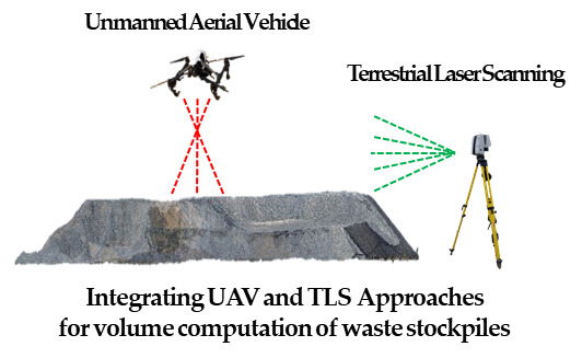
In this study, we compared and fused the TLS and UAV technologies by analyzing their spatial features and efficiencies. The specific objectives of this study were to (1) build point clouds using the TLS and UAV technologies, (2) perform waste stockpile volume computations to derive an optimal computation technique based on technology fusion, and (3) present a comparative analysis of these technologies.
2. Materials and Methods
First, we separately built two point clouds using TLS and UAV technologies, evaluated their accuracies, and performed waste stockpile volume computations. For the UAV investigation, we set up various scenarios and performed volume computation for the scenario yielding the most accurate point cloud. A variety of scenarios were set up for the UAV because different flight designs were required to estimate the effect of the number of GCPs and their placement on model accuracy [
23,
31,
32]. Then, we conducted a comparative spatial analysis of the TLS and UAV technologies and performed waste stockpile volume computations via a TLS/UAV fusion model. Finally, we analyzed the volume computation results.
For the UAV technology, we used DJI Inspire 1 Pro (Shenzhen, China), a rotary-wing UAV resistant to wind and capable of flying for approximately 15 min. Since a single mission was unable to cover the entire study area, a sufficient number of batteries were prepared for repeated mission flights. For image acquisition, we used a camera sensor (ZENMUSE X5) (Shenzhen, China) with 16 megapixels and a 72° diagonal field of view.
For TLS, we used a Leica ScanStation P40 (Aarau, Switzerland) with an ultra-high scan rate of 1,000,000 points/s at a maximum range of 270 m. The GNSS survey was performed using a Trimble R8s GNSS receiver (Sunnyvale, California, USA) to enhance the positional accuracies of point clouds and evaluate the accuracy of each point cloud. The R8s is equipped with 440 channels and supports GPS and global navigation satellite system (GLONASS) satellites. Image processing and GNSS survey data points were processed separately using the Pix4D Mapper 4.3 (Prilly, Switzerland), Cyclone 9.2.1 (Aarau, Switzerland), CloudCompare 2.10.2 (Aarau, Switzerland), and ArcMap 10.1 (California, Redlands, USA) software.
The accuracy of TLS- and UAV-based point cloud data was compared using the model-to-model cloud comparison (M3C2) algorithm, and the UAV-based point cloud efficiency was evaluated based on the UAV flight time, GCP, and control point (CP) measurement time. The individual steps of the process are described in
Section 2.2,
Section 2.3 and
Section 2.4.
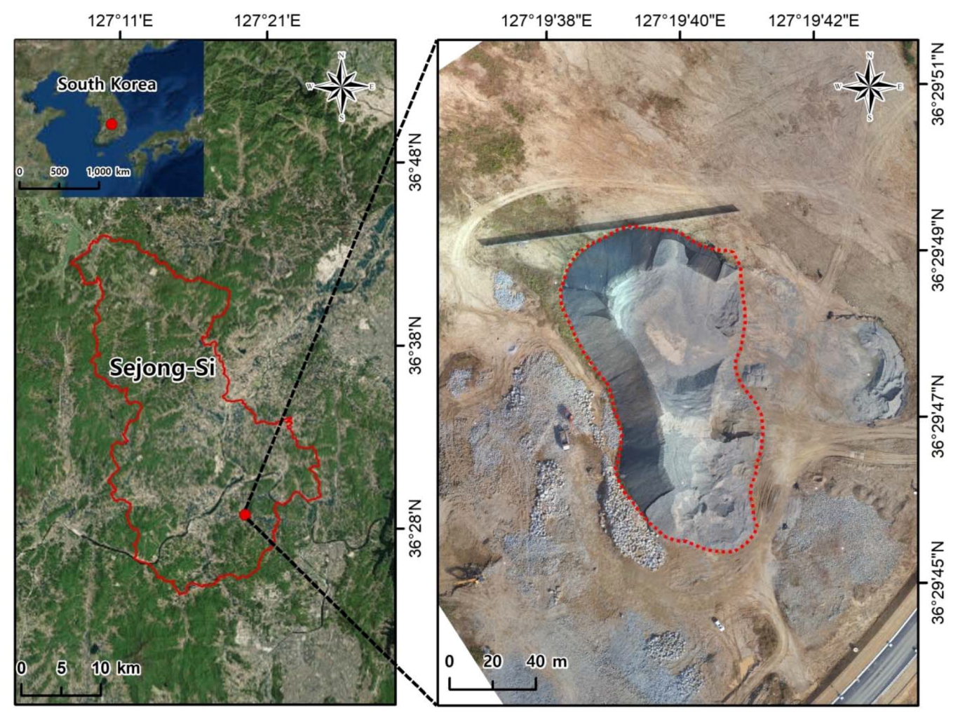
2.1. Study Area
A site for waste stockpiles in Jipyeon-ri in Sejong City, South Korea was selected as the study area. Sejong City is a planned city in which large construction sites and residential areas coexist. Excavated earth materials and construction wastes are stored at a temporary waste disposal site, damaging the landscape and posing problems to residential areas via wind-blown dust. Construction site waste management is, therefore, a compelling issue, and accurate waste volume computation is important for the waste removal plan. The waste disposal site selected as the study area extends over ~6000 m
2, containing a significant volume of waste, which is challenging to measure. The peak waste mound height is approximately 20 m spreading over a 130 m × 90 m surface area. Wastes are mostly from construction sites and include concrete, slag, and sand. Due to the limited access to the mound featuring uneven surfaces, measurements were taken using a ladder in this study (
Figure 1).
2.2. TLS- and UAV-Based Point Cloud Generation and Waste Stockpile Volume Computation
The UAV images and TLS measurements were taken on 10 October 2018. UAV images were taken from 10 a.m. to 11 a.m., whereas TLS measurements were conducted from 2 p.m. to 4 p.m. The temperature and humidity data provided by a nearby weather station on 10 October 2018 were 16.3 °C and 49.5% at 10 a.m. and 15.9 °C and 34.8% at 4 p.m., respectively.
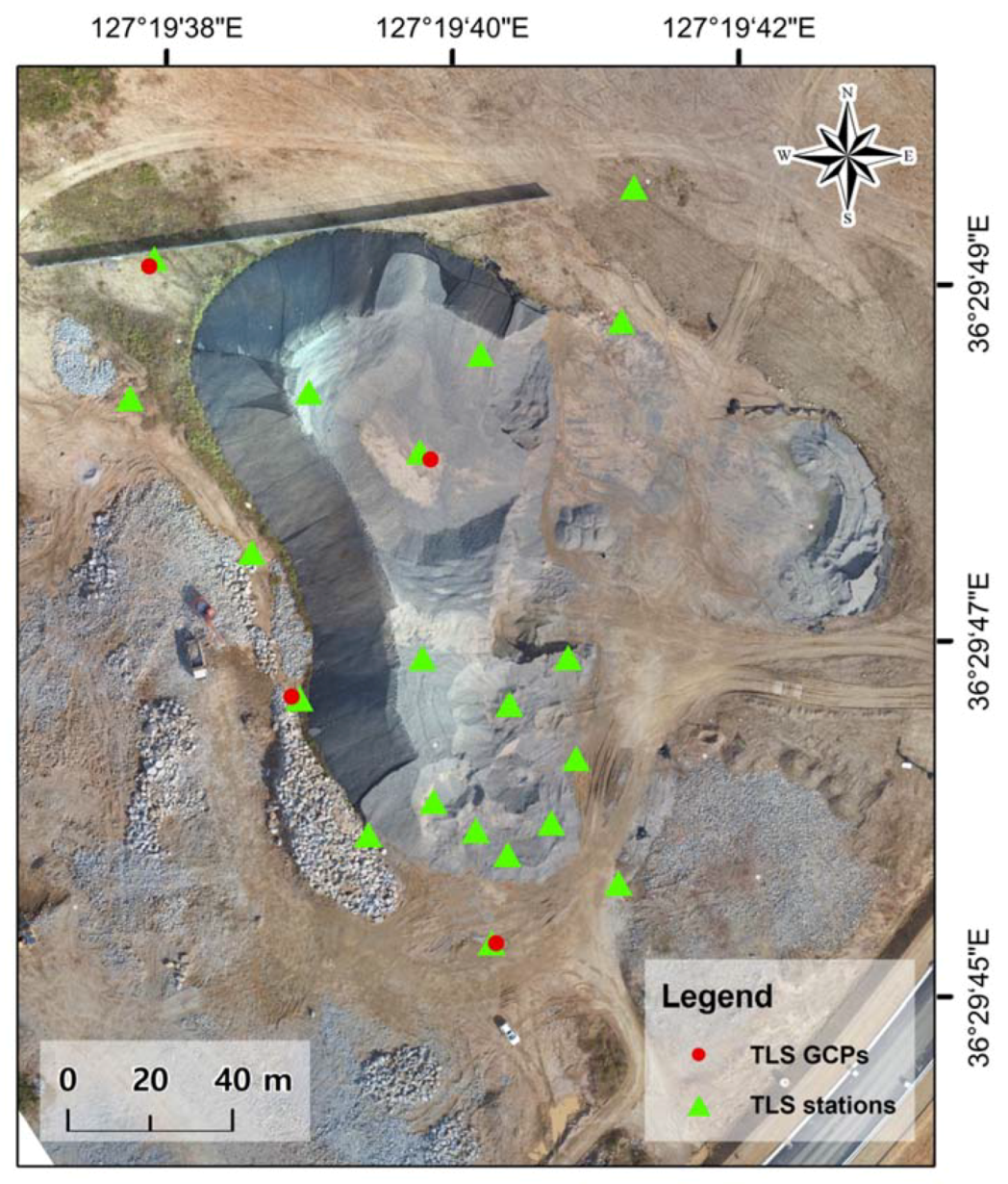
The overall process of TLS-based point cloud generation can be divided into three phases. (1) In the goal setting and planning phase, the scan positions and distances should be planned to account for shadow zones and disturbances. (2) In the field scanning phase, scanning is performed based on the planned scan positions, and backups are executed to prevent data loss. The quality of the scanned data is verified during scanning such that rescanning is performed if necessary. In this study, field scanning was conducted at 20 scan positions (
Figure 2). To ensure accurate registration of individual scan data, GCPs should be measured in the survey area and the measured values should be reflected in the ensuing data processing. This study used four GCPs. (3) In the data processing phase, the datasets acquired in the field scanning phase are registered and converted into georeferenced coordinates. The converted data points are realigned and unnecessary parts are removed.
Data processing was performed using the Cyclone 9.2.1 software and accuracy evaluations and volume computations were conducted using CloudCompare 2.10.2 and ArcMap 10.1, respectively.
To implement the UAV-based point cloud generation, we set the flight altitude, image overlap, and number of GCPs as key parameters. The flight plan must be scrutinized and set up accordingly because the data for a particular location of interest may not be shown otherwise, forcing a return to the recovery point [
33].
The flight altitude was varied from 40 to 160 m (in 40 m intervals). A higher flight altitude can decrease the flight time by reducing the number of images required to cover the survey area, but it results in a larger ground sampling distance, i.e., lower image resolution and quality. Therefore, the flight height was set to four different levels, accounting for the height of the waste pile in the survey area.
The three-dimensional (3-D) vision is only possible when at least two images overlap, and the overlap ratio is typically set at 60–80% [
34,
35] or 80% for cities with complex landscapes [
34]. Greater image overlap can enhance the quality of image registration results, but it requires more flight and data processing time. We set a fairly high overlap rate in this study, i.e., 85% forward lap (FL) and 65% side lap (SL).
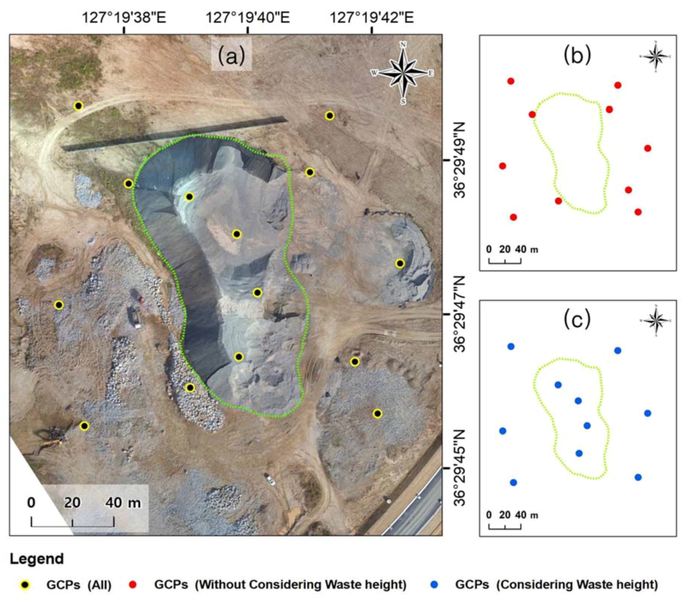
The number of GCPs is an important parameter related to image quality. Numerous studies have attempted to explain the relationship between the number of GCPs and image quality enhancement. In [
36], one GCP per 2 ha yielded the highest accuracy, while [
37] highlighted the importance of an even GCP distribution across the survey area. In this study, we also examined the association between the number of GCPs and point cloud accuracy by setting a sufficient number of GCPs based on previous studies. We conducted two surveys (i.e., one that included the waste pile and one that excluded it) in two GCP placement scenarios, placing 10 GCPs across each survey area (
Figure 3). This GCP placement criterion is different from that in previous studies in which the number of GCPs or their even distribution was more important. We used a different criterion to test our hypothesis that the altitude-dependent GCP placement influences image quality.
Data processing was performed using the Pix4D Mapper 4.3 software, and accuracy evaluations and volume computations were conducted using CloudCompare 2.10.2 and ArcMap 10.1, respectively. Volume computation was performed using the following equation:
where
Li,
Wi, and
Hi are the length, width, and height of the cell, respectively [
38]. The height of the cell is the difference between the terrain altitude of the cell given at its center and the base altitude in the cell’s center, defined as follows [
38]:
where
ZTi is the altitude in the center of cell
i of the 3-D terrain and
ZBi is the altitude in the center of cell
i from the base surface [
38].
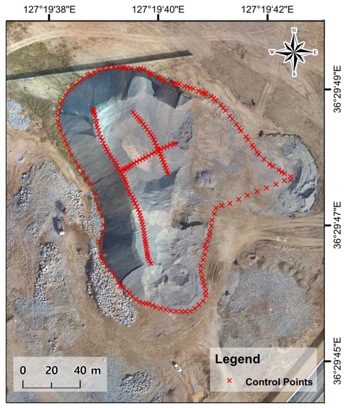
The accuracy of the point clouds generated using the TLS and UAV technologies was evaluated by comparing them with those generated by setting a large number of control points (CPs) in the survey area based on a GNSS field survey. The discrepancy between the 3-D model and CPs can be used to evaluate the model accuracy using the root mean square error (RMSE). The RMSE is a statistical metric commonly used to validate the accuracy of point cloud-based modeling approaches such as TLS and UAV [
31,
39]. The RMSE is a popular and easily understood proxy when the “ground truth” dataset is a set of distributed points rather than a continuous “truth” surface [
21]. In this study, CPs were measured with the VRS/RTK-GNSS in Trimble R8s. In total, 311 CPs were measured, as shown in
Figure 4.
Measurements were performed at CPs located across the study area, generating reference data essential for evaluating the point cloud accuracy. The RMSE reflects the accuracy of each of the
x,
y, and
z components, but we computed the RMSE using the
xyz value, which was obtained by combining the RMSEs corresponding to
x,
y, and
z, as follows:
where
RMSEx can be defined as follows:
where Δ
xi is the difference between the CP coordinates and coordinates determined from the point cloud and
n is the number of points. The same equation applies to
RMSEY and
RMSEZ mutatis mutandis.
2.3. Comparison of Spatial Features and Efficacy of Point Clouds
We compared the point clouds generated using the two previously discussed technologies by analyzing their spatial features and efficiencies. Three techniques are generally used when comparing two spatial models, namely the DEM of difference (DoD), direct cloud-to-cloud (C2C), and cloud-to-mesh or cloud-to-model distance (C2M) techniques [
40,
41]. However, these methods have disadvantages when used to compare point clouds, which are summarized as follows.
The DoD method, which is used to compare two DEMs, cannot handle overhanging, such that information density decreases in proportion to surface steepness [
39]. Moreover, it is not a full 3-D model, but rather a 2.5-D model in which
z is added to a cell, rendering it unsuitable for evaluating the complex morphology of solid waste [
42].
The C2C approach is the simplest and fastest direct method for a 3-D comparison of point clouds [
43]. For each point of the second point cloud, the closest point can be defined in the first point cloud. In its simplest version, the change in the surface can be estimated as the distance between the two points. However, this method cannot be used to calculate spatially variable confidence intervals [
41].
In the C2M method, the change in the surface can be calculated based on the distance between a point cloud and a reference 3-D mesh [
44], which generally requires time-consuming manual inspection. As in the DoD technique, interpolation of missing data introduces uncertainties that are difficult to quantify [
41].
To overcome the uncertainties associated with the spatial data comparison, we can use the M3C2 algorithm [
41], which enables the rapid analysis of point clouds with complex surface topographies [
40,
41,
45]. The M3C2 algorithm finds the best-fitting normal direction for each point and then calculates the distance between the two point clouds along a cylinder of a given radius projected in the normal direction [
46]. Barnhart and Crosby [
40] divided the M3C2 algorithm into two steps—point normal estimation and difference computation. Users may specify if local point normals are calculated or if normals are fixed in either the horizontal or vertical direction [
40]. Horizontal point normals allow true horizontal erosion rates to be calculated from the M3C2 analysis, whereas vertical normals allow M3C2 data to be used for strictly vertical erosion and aggradation measurements [
40]. In this study, point cloud comparison was performed using the M3C2 algorithm instead of a conventional spatial model comparison technique.
For efficiency analysis, we employed the time variables used by Silva et al. [
30] when comparing the UAV, GNSS, and LiDAR and those used by Son et al. [
47] when building a UAV-based DSM. The efficiency and accuracy were compared by analyzing the time required for point cloud generation based on the UAV and TLS technologies. For the UAV case, we selected the scenario with the highest accuracy.
2.4. Point Cloud Fusion and Volume Computation
We built one point cloud by fusing the TLS- and UAV-based point clouds to compare the spatial accuracy and efficiency of the TLS-UAV fusion model with those of each individual model. Although higher accuracy is expected for the point cloud generated using the fusion model, efficiency of the process should also be considered. We fused the two technologies and analyzed the performance of the fusion method to test the hypotheses that the TLS- and UAV-based point clouds have their respective problems, which can be solved by point cloud generation using a fusion of these two technologies. As the UAV-based point cloud, we selected the most accurate cloud from among the eight point clouds generated in eight different scenarios.
The fused TLS- and UAV-based point cloud equation can be expressed as follows:
where
is the TLS-based point cloud,
is the UAV-based point cloud, and
is the fused TLS- and UAV-based point cloud.
The TLS- and UAV-based point clouds were fused using the CloudCompare 2.10.2 software. Since the point clouds use the same coordinate system (Korea 2000/Central Belt 2010–EPSG:5186), there is no need to perform additional georeferencing. The volume computation accuracy of the point cloud generated by the fusion approach was evaluated using the same method employed for the TLS and UAV methods.
3. Results
3.1. Point Cloud Generation and Volume Computation
TLS-based point cloud data were obtained by scanning the survey area from all 20 scan positions. The individual scan data were registered into a single point cloud, yielding reasonably high accuracy (RMSE = 0.202 m). The volume computed using the TLS-based point cloud was 41,226 m3.
UAV-based point clouds were generated for eight scenarios (A–H), with four flight altitudes and two sets of 10 GCPs as variables (
Table 1).
Among eight scenarios (A–H) in which point clouds were generated, scenario A was the most accurate one (RMSE = 0.032 m). Scenario A was configured with a flight altitude of 40 m and a set of 10 GCPs considering the waste height. In scenarios considering waste height (A, C, E, and G), the RMSE increased with the increasing flight altitude, which indicates that accuracy has an inverse correlation with flight altitude. In scenarios with evenly distributed GCPs (B, D, F, and H) that did not consider waste height, no correlation was observed between the RMSE and flight altitude.
Volume computation was conducted on eight UAV flight scenarios using the corresponding point clouds (
Table 2).
Among eight scenarios (A–H) in which volume computation was performed, those with GCPs placed atop the waste pile (A, C, E, and G) exhibited similar values (~41,000 m3). This finding can be examined in association with the RMSE. The computed volumes for the other scenarios (B, D, F, and H), which did not have high point cloud accuracy, deviated considerably from each other. Such observations are attributed to the fact that volume is obtained from point cloud data comprising x, y, and z values. In other words, x, y, and z coordinates must be sufficiently accurate to reduce the estimated volume uncertainty.
3.2. Comparison of Spatial Features and Efficacy of Point Clouds
The M3C2 algorithm was employed to compare and analyze the point clouds generated using the TLS and UAV technologies. For UAV-based point clouds, scenario A, which had the highest accuracy, was used. Although both the TLS and UAV methods yielded point clouds with fairly high accuracies, they had certain drawbacks.
Figure 5a,b shows the side-view images comparing the TLS- and UAV-based point clouds of the waste disposal site.
Figure 5a-1,b-1 depicts the point clouds generated using the TLS approach, whereas
Figure 5a-2,b-2 presents those obtained using the UAV method. The latter two images show missing portions, presumably due to the difference between the TLS position and UAV shooting position. The TLS technology scans sideways from positions fixed on the ground, but UAV images taken from above are more likely to miss side-view aspects. Constructing a model similar to the original shape is possible using SfM algorithms, with images taken from different positions as configured when setting the UAV flight parameters. However, this technique was not sufficient to reproduce irregularly curved sides.
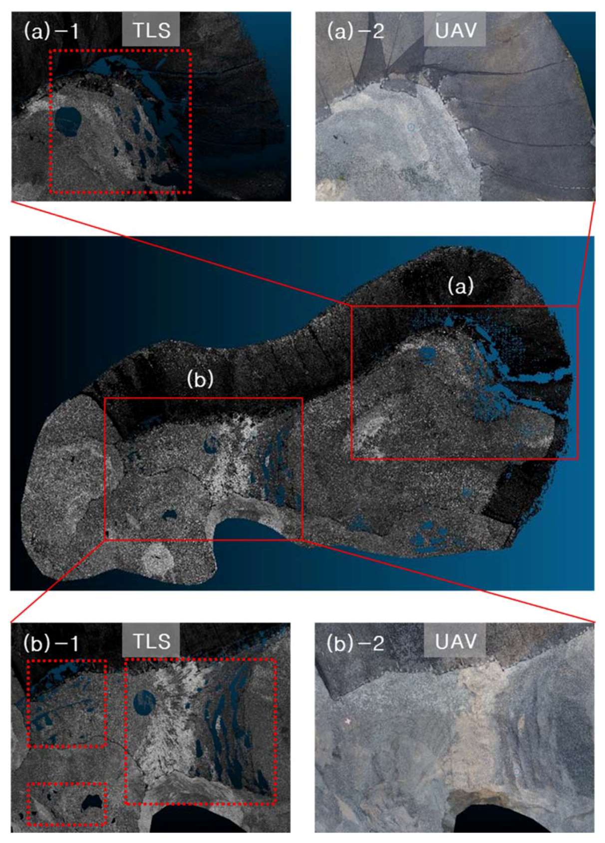
Figure 6a,b shows the top-view images comparing the TLS- and UAV-based point clouds of the waste disposal site.
Figure 6a-1,b-1 presents the images of the TLS-based point cloud, whereas
Figure 6a-2,b-2 depicts the UAV-based point cloud. Although TLS was also performed on top of the waste pile, the TLS-based point cloud exhibits unskinned portions, presumably due to uneven surfaces with steps and grooves. The TLS method was particularly prone to errors when representing grooves in the point cloud. In contrast, grooves and curves were well reflected in the UAV-based point cloud. In addition to the advantage of the UAV’s vertical shooting position in taking top-view photos, as mentioned in the side-view image discussion, the GCPs placed atop the waste pile presumably contributed to the representation accuracy.
We then calculated the time required to generate a point cloud, i.e., from the beginning of the TLS and UAV flight to point cloud completion, to compare the time requirements of the TLS and UAV technologies (
Table 3).
The TLS and UAV methods required 800 and 340 min, respectively. The same amount of time was spent measuring CPs, which were used for accuracy evaluation, because the same data were used for TLS and UAV tests. TLS required more time, with the exception of the time spent measuring the GCPs. Given the small size of wastes in the study area compared to the typical volumes of disaster and construction wastes, the feasibility of using TLS technology for volume computation is considered low.
3.3. Point Cloud Fusion and Volume Computation
We then built a single point cloud by fusing the TLS- and UAV-based point clouds. The fusion model yielded the following values: RMSE = 0.030 m and volume = 41,232 m
3 (
Table 4).
The point cloud accuracy of the fusion model was higher than those of the TLS and UAV methods, but similar to that of the UAV method. Müller et al. [
29] constructed a high-resolution DEM by fusing TLS and UAV technologies to monitor an eruption site. Although a fusion model was used to reflect the geomorphological characteristics of the study area, comparisons and analyses showed that the UAV approach alone can yield the desired results.
4. Discussion
The accuracy of UAV-based point clouds was evaluated for each scenario. In general, a lower flight height enhances image resolution and allows for more images to be taken with overlapping parts, resulting in higher image quality and accuracy. However, no significant effect of the flight altitude was observed when the GCPs were placed only on flat land. This finding suggests that the GCP arrangement is associated with the accuracy of the point cloud model [
31,
48,
49]. Most studies, which have been conducted in areas with only slight elevation variations, have mostly focused on the number of GCPs, rather than on their placement [
13,
50]. The results of this study demonstrate that GCPs should also be placed at the highest points in an area with significant elevation variations.
Although the UAV method outperformed the TLS approach in terms of point cloud accuracy, this finding does not necessarily indicate that UAV technology is superior to TLS technology. In the UAV approach, an optimized point cloud can be built by selecting the best performing scenario among eight different scenarios. If the TLS method was conducted using a similar experimental setup (i.e., with more scan stations and more elaborate measurements), its accuracy would have also improved. Jo and Hong [
5] built point clouds of the same target object using TLS and UAV technologies, computing the accuracies of the
x,
y, and
z coordinates. The TLS approach yielded more accurate
x and
y coordinates, whereas the UAV method generated slightly more accurate
z coordinates. There remains considerable room for discussion regarding the performance of these two techniques in terms of time, cost, and efficiency.
In the TLS/UAV point cloud fusion model, the TLS and UAV technologies can mutually compensate for the disadvantages of each other. Although TLS is advantageous over UAV technology when surveying a small area (in terms of image accuracy), it has limitations in surveying large areas [
51]. Jo and Hong [
5] suggested that, in the fusion of the UAV- and TLS-based point clouds of an area with buildings and surrounding grounds, a UAV can be employed to obtain the point cloud at the top of the building, which is difficult to obtain via TLS, thereby enhancing the overall accuracy of the 3-D point cloud data.
In this study, we applied the TLS and UAV methods to the sides and top of the waste pile, respectively, and showed that the integrated use of TLS and UAV technologies can compensate for the drawbacks of each method. However, given the insignificant difference in accuracy between the UAV- and fusion model-based point clouds, the efficacy of these methods should be further examined. The total time spent on point cloud generation was 800 min for TLS and 340 min for the UAV. The fusion model required considerably more time because of its own analysis time in addition to the time taken for the TLS and UAV approaches. Consequently, the UAV method alone can be considered highly advantageous in terms of efficiency.
In summary, the fusion model may be a rational solution to the problems associated with UAV and TLS technologies, but it is less efficient than the UAV approach. The UAV method is prone to errors in side-view photogrammetry during point cloud generation, which can be overcome by UAV tilt control and flying along the sides of a waste pile. The insufficient representation of the sides in a point cloud obtained in this study is ascribable to the limitation of the vertical UAV shooting position. In view of this insufficiency, future research must focus on deriving an optimal configuration of various flight parameters, such as the camera position and direction, to enhance the accuracy of point cloud generation and volume computation.
The present study estimated the waste volume from the environmental management perspective and requires further discussion from the temporal standpoint. Wastes from mass developments or natural disasters must be quantified and examined in a timely manner for proper management. Large-scale wastes from mass developments must be processed within a predefined time period according to the Environmental Impact Assessment Act, while those from natural disasters must be quickly quantified to prevent subsequent damage. In light of this, the UAV-based volume estimation method exhibits relatively high accuracy and shorter processing time; it can therefore be applied in a variety of situations wherein fast and accurate volume estimation is critical.
5. Conclusions
Continuous monitoring of developing project sites is essential to minimize environmental problems resulting from long-term stacking of waste stockpiles, such as scattered dust and soil loss. Three volume computation methods (TLS, UAV, and TLS/UAV) were compared and analyzed in this study to obtain accurate volume estimates that must precede continuous monitoring activities. Waste stockpile volume computations were performed using the generated point clouds, and the accuracy and efficacy of the three techniques were compared.
All three techniques were suitable for generating highly accurate point clouds. The fusion model was the most accurate one, followed by the UAV and TLS approaches, with the point cloud accuracy of the fusion model being similar to that of the UAV method. Similar volumes were computed using all three techniques. The UAV-based volume estimation method was the most effective one in terms of time requirement, whereas the fusion method yielded the most accurate results (
Table 5).
Although the UAV approach is advantageous for rapidly performing waste stockpile volume computations in a large area, the UAV and TLS technologies can mutually compensate for their respective weaknesses in capturing images through scanning or aerial photography, depending on the situation and target object. The fusion method exploits the advantages of both UAV and TLS. This method is deemed appropriate for historical objects requiring a more detailed point cloud rather than for reconstruction and preservation of forestry where the point cloud generation at the lower end of the forest is challenging [
28,
52].
Future studies should determine the most efficient method of computing the volumes of solid waste stockpiles at different scales by considering the time requirements and economic factors, such as equipment and labor costs. Research on topographic point cloud generation with a LiDAR sensor mounted on a UAV is ongoing and will enable point cloud generation with a higher density than UAV photogrammetry [
53]. Thus, we should also perform volume computations using a UAV camera and UAV LiDAR, followed by a comparison of their performance. The results of this study demonstrate that efficient environmental management can be achieved using UAVs for environmental impact assessments or environmental monitoring associated with large-scale development projects.


