Abstract
Confidence in the use of Earth observations for monitoring essential climate variables (ECVs) relies on the validation of satellite calibration accuracy to within a well-defined uncertainty. The gap analysis for integrated atmospheric ECV climate monitoring (GAIA-CLIM) project investigated the calibration/validation of satellite data sets using non-satellite reference data. Here, we explore the role of numerical weather prediction (NWP) frameworks for the assessment of several meteorological satellite sensors: the advanced microwave scanning radiometer 2 (AMSR2), microwave humidity sounder-2 (MWHS-2), microwave radiation imager (MWRI), and global precipitation measurement (GPM) microwave imager (GMI). We find departures (observation-model differences) are sensitive to instrument calibration artefacts. Uncertainty in surface emission is identified as a key gap in our ability to validate microwave imagers quantitatively in NWP. The prospects for NWP-based validation of future instruments are considered, taking as examples the microwave sounder (MWS) and infrared atmospheric sounding interferometer-next generation (IASI-NG) on the next generation of European polar-orbiting satellites. Through comparisons with reference radiosondes, uncertainties in NWP fields can be estimated in terms of equivalent top-of-atmosphere brightness temperature. We find NWP-sonde differences are consistent with a total combined uncertainty of 0.15 K for selected temperature sounding channels, while uncertainties for humidity sounding channels typically exceed 1 K.
1. Introduction
The exploitation of geophysical information from earth observation (EO) space borne instruments, particularly where quantifying uncertainties is important, depends on the calibration and validation of these data to a recognized standard. This user requirement has led to the development of various validation practices in EO communities [1]. Methods for post-launch characterization include dedicated field campaigns [2,3], vicarious calibration against invariant ground targets [4], simultaneous nadir overpasses (SNOs) for intercalibration [5], and double differences via a third transfer reference [6], although these all suffer to some extent from limited sampling.
The framework of numerical weather prediction (NWP) is attractive for assessment of satellite instrument performance, since NWP forecast and reanalysis models ingest large volumes of observational data and offer comprehensive spatial and temporal sampling. Modern data assimilation (DA) systems blend information from observations and the forecast model to arrive at an optimal estimate (analysis) of the atmospheric state. Model physics constraints ensure that the resulting global atmospheric fields are physically consistent. NWP forecasts are routinely validated by comparison with reference observations (e.g., radiosondes) or NWP analyses, and accurate representations of three-dimensional temperature and humidity fields make NWP systems effective in detecting subtle artefacts in satellite data [7,8,9,10,11].
It is routine at NWP centers to compare satellite observations with model equivalents. To perform such an assessment, NWP fields at the time of observation are transformed into radiance space using a fast radiative transfer model. The diagnostic for the comparison is then the observation minus short-range forecast (“background”) fields in radiance space, termed O-B or background departure. O-B differences may be systematic (apparent as large-scale global biases), geographically local, or random (e.g., resulting from satellite instrument noise). The instrument state dependence and geophysical state dependence of biases can be used to infer the mechanisms underlying these differences (e.g., sensor calibration errors, NWP model forecast errors or radiative transfer errors).
The European Union gap analysis for integrated atmospheric ECV climate monitoring (GAIA-CLIM) project investigated the calibration/validation (cal/val) of satellite data sets using non-satellite reference data. During the three-year project the potential of NWP frameworks for assessing and validating new satellite missions was explored. DA systems employed operationally by two independent forecasting centers, the European Centre for Medium-Range Weather Forecasts (ECMWF) and the Met Office, were used to evaluate a number of recently launched satellite sensors.
NWP model data are not yet traceable to an absolute calibration standard. Activities within GAIA-CLIM aimed to develop the necessary infrastructure at NWP centers for the routine monitoring of reference networks such as the GCOS (global climate observing system) reference upper-air network (GRUAN) in order to establish a traceable linkage between NWP and reference standards. As a result the GRUAN processor was developed [12] to collocate GRUAN radiosonde profiles and NWP model fields, simulate the top-of-atmosphere brightness temperature at frequencies used by space-borne instruments, and propagate uncertainties to gauge the statistical significance of NWP-GRUAN differences.
In this paper, we explore the use of NWP as a reference for satellite cal/val. We present results of comparisons between NWP and satellite data from a number of recent missions where the NWP fields were particularly useful in identifying anomalies in satellite measurements. We show we can attribute O-B signatures to instrument calibration biases or external influences such as radio frequency interference. We further investigate the absolute uncertainty in the NWP fields using the GRUAN processor. Finally, we discuss whether NWP fulfills the validation requirements for the upcoming MetOp second generation temperature and humidity sounding missions.
2. Materials and Methods
2.1. NWP Assessments of Current Satellite Missions
It is modern practice at NWP centers to assimilate satellite radiances, in preference to products retrieved from the radiances such as temperature and humidity profiles. A fast radiative transfer model is required to map between radiances and Earth system variables, for which the Met Office and ECMWF use radiative transfer for TOVS (RTTOV) [13].
ECMWF and the Met Office have implemented a four-dimensional NWP data assimilation system (4D-Var) [14,15]. The Met Office also employs a simplified 1D-Var pre-processing step [16]. Using vector notation, we represent the atmosphere and surface variables on which the radiances depend as a state vector x and compute the simulated satellite radiance H(x) for RTTOV observation operator H. The 1D-Var assimilation, which is analogous to that performed within the full 4D-Var system, proceeds by minimizing the cost function
in order to estimate the most probable solution for x. Here, is the a priori background vector from the NWP forecast model, y is the vector of measurements (radiances for satellite channels of interest), while B and R represent the error covariance characteristics of the NWP background state and observations respectively.
The difference between the observations and NWP model background (O-B) is the key parameter we use as a diagnostic in this paper. We examine the characteristics of these departures and seek to determine their dependence on geophysical and/or instrument variables.
2.1.1. Satellite Data Description
Several satellite instruments were assessed in coordinated activities at the Met Office and ECMWF during the GAIA-CLIM project as summarized in Table 1. Three of these sensors are conically scanning instruments with channels at frequencies below 90 GHz. The advanced microwave scanning radiometer 2 (AMSR2) on the global change observation mission–water satellite 1 (GCOM-W1) is a follow-on from previous Japan Aerospace Exploration Agency (JAXA) missions AMSR and AMSR-E. Several major changes have been made to improve the AMSR2 design [17]. These include a larger main reflector, thermal design changes to address temperature non-uniformities, and extensive sunlight shielding. A hot load calibration target and cold sky mirror are used for two-point radiometric calibration. The reflector rotates to provide Earth views with a fixed incidence angle of 55°. AMSR2 has fourteen channels (seven frequencies with dual polarization between 6.9 GHz and 89 GHz).

Table 1.
Passive microwave satellite sensors assessed within the NWP framework in this study. GCOM-W1 was launched in May 2012; FY-3C was launched in September 2013; GPM was launched in February 2014.
The MicroWave Radiation Imager (MWRI) and MicroWave Humidity Sounder -2 (MWHS-2) instruments fly on the Chinese FengYun-3C (FY-3C) polar orbiting satellite. MWRI is a microwave conical-scanning imager with 10 channels at frequencies ranging from 10.65 GHz to 89 GHz which are sensitive to total column water vapor, cloud and precipitation. A 3-point calibration method is used for MWRI, involving the use of three reflectors. Antenna nonlinearity corrections for MWRI were suggested to be the largest source of calibration uncertainty [18]. MWHS-2 scans cross-track and has 8 channels which sample around the 118.75 GHz oxygen line, 5 channels sampling the 183 GHz water vapor line, and 2 window channels at 89 GHz and 150 GHz. Results from pre-launch tests indicated calibration uncertainties of around 0.3 K for most channels [19].
The global precipitation measurement (GPM) mission is the result of an international effort led by NASA and JAXA built on the tropical rainfall measuring mission (TRMM) legacy. The satellite flies in a non-Sun-synchronous orbit that provides coverage of the Earth from 65°S to 65°N. The GPM Microwave Imager (GMI) has 13 channels ranging in frequency from 10.65 GHz to 183.31 GHz. Its design benefits from a number of enhancements over its heritage from the TRMM Microwave Imager (TMI) and other similar instruments. The main reflector has an improved low emissivity coating, the instrument design mitigates against solar intrusions and thermal gradients and additional calibration points are provided via internal noise diodes for low-frequency channels up to 37 GHz [20,21]. One study [22] estimated the absolute calibration accuracy to be within 0.25 K root mean square error, supporting the design goal of GMI to be the GPM calibration standard.
2.1.2. Data Assimilation Configurations
At ECMWF, a hybrid incremental 4D-Var assimilation model is used with a 12-h assimilation window. The forecast model used in operations has a resolution of TCo1279 (approximately 9 km horizontal resolution, 137 vertical levels). For the purpose of monitoring satellite data for GAIA-CLIM the experiments have a reduced resolution of TCo399 (approximately 25 km, 137 levels). ECMWF employs an all-sky scheme to assimilate microwave radiances over ocean [23,24]. In order to account for the scattering, emission, and absorption effects of cloud and precipitation, ECMWF uses a version of RTTOV known as RTTOV-SCATT [25].
At the Met Office the assimilation proceeds in two stages. At N768L70 resolution (~25 km horizontal resolution at mid-latitudes, 70 vertical levels from the surface to 80 km), a 1D-Var retrieval is performed for quality control and to derive physical parameters which are subsequently fixed in the full incremental 4D-Var assimilation across a 6-h time window. For this study, we have used the output from the Met Office 1D-Var preprocessor without recourse to running the more computationally expensive 4D-Var. This means the model background used to calculate O-B departures is a short-range forecast of typically a few hours. The Met Office uses the non-scattering version of RTTOV but includes the absorption effects of cloud liquid water. Since the work presented here, the Met Office forecast model has been upgraded to N1280L70 resolution, corresponding to a grid length of approximately 10 km at mid-latitudes.
Both centers produced statistics for this study without applying bias corrections to the satellite data as is done operationally. These are presented over ice-free, open ocean only, since the surface emissivity and skin temperature required as input to RTTOV is considered more accurate than over land or sea ice. ECMWF and the Met Office use the fast microwave emissivity model (FASTEM) [26,27] over ocean.
Wherever possible, differences in the treatment of observations at ECMWF and the Met Office were minimized. However, for technical reasons the centers’ configurations differed in minor respects. RTTOV version 11 was used at both centers for the intercomparison, with the exception of the FY-3C MWHS-2/MWRI study at the Met Office for which RTTOV version 9 was used. FASTEM-6 was used throughout at ECMWF. The Met Office processed data for this paper using FASTEM-6 except for MWHS-2 where FASTEM-2 was used.
2.1.3. Data Selection
In this study we aim to analyze O-B statistics such that the model simulated radiances are as reliable a reference as possible. Therefore, we should select cases where the NWP model background state exhibits small errors and the radiative transfer model is capable of accurately representing that model state in radiance space. There are some meteorological regimes that are problematic in this regard, such as the presence of clouds and precipitation for which the NWP forecast model may be in error spatially and temporally, and for which the radiative transfer is complicated. By contrast, in clear skies, we expect the NWP model state of temperature and (to a lesser extent) humidity to be accurate for short forecast lead times, and the radiative transfer to be simpler than for cloudy skies.
At ECMWF cloudy microwave imager observations are assimilated by varying the weight given to observations as a function of an effective cloud amount [28] derived from the observations and the background. For microwave imagers the normalized polarization difference at 37 GHz is used [29,30]:
where and are the 37 GHz V- and H-polarized brightness temperatures respectively, and are the all-sky background brightness temperatures for these channels (calculated using RTTOV-SCATT), and and are the clear-sky background brightness temperatures for these channels neglecting cloud effects. At 37 GHz the sea-leaving radiance is highly polarized, while contributions due to clouds or precipitation tend to be unpolarized. Thus, we expect and to vary between 1 in clear sky conditions and 0 in conditions of total opacity. We can define an effective cloud amount as
We can now apply a cloud screening where we include observations only for low effective cloud amounts:
We keep AMSR2, MWRI, and GMI data for analysis only where both tests (6) and (7) above are met. The threshold value of 0.05 is a compromise between retaining sufficient observations to be globally representative and ensuring the quality control is strict. The Met Office does not currently use RTTOV-SCATT in operations. For this study RTTOV-SCATT was run offline using Met Office background fields in order to estimate and .
For MWHS-2 we use a scattering index (we calculate whether the difference between brightness temperatures at 89 GHz and 150 GHz exceeds a threshold) to screen out observations affected by scattering from precipitation and cloud ice.
A criterion was used to accept observations only within the range 60°S to 60°N in order to avoid sea ice contaminated data, except for MWRI where the range was 50°S to 50°N. Some data usage details differ between ECMWF and the Met Office. At ECMWF, AMSR2, MWRI and GMI data are spatially averaged over 80 km scales (“superobbed”) while individual footprints are assimilated at the Met Office. However, for MWRI only superobbing was switched off at ECMWF to improve consistency with Met Office data. An additional screen was applied to ECMWF statistics to remove data in cold-air outbreak regions because such regions have been shown to exhibit systematic biases between model and observations [31]. A complete description of the quality controls used in the two centers’ frameworks can be found in publicly-available GAIA-CLIM reports [32,33,34].
2.2. The GRUAN Processor
NWP-based cal/val assessments of satellite data have been hampered to date by the lack of metrologically traceable characterization. The evaluation of errors and uncertainties in NWP model fields was addressed during GAIA-CLIM by the development of the GRUAN processor [12]. GCOS (Global Climate Observing System) reference upper-air network (GRUAN) radiosondes are processed following strict criteria, correcting for known sources of error and reporting uncertainty estimates for profiles of temperature, humidity, wind, pressure and geopotential height [35]. GRUAN uncertainties do not include error covariance estimates. The GRUAN processor collocates GRUAN radiosonde profiles and NWP model fields to facilitate a comparison of the pairs of profiles. Importantly, the NWP-GRUAN comparison is performed in radiance (or brightness temperature) space using RTTOV to simulate the top-of-atmosphere radiance from the radiosonde and model profiles. In this way NWP fields can be compared with reference GRUAN data for any sensor RTTOV is able to simulate. The unique solution offered by a forward radiative transfer calculation avoids the ambiguity that is inevitable in inverse calculations (retrievals). The GRUAN processor also allows profile uncertainties to be mapped to observation space for a meaningful comparison. This is achieved by applying RTTOV Jacobians to matrices representing sources of uncertainty [12].
2.2.1. Sampling for GRUAN Comparison
For this study GRUAN profiles from nine sites were collocated with ECMWF and Met Office fields for the six-month period July-December 2016. We divide the sites into three geographic regions (Table 2).
Table 2.
Details of GRUAN sites used in this study.
The GRUAN processor generated NWP-GRUAN comparisons for all GRUAN radiosonde ascents during the period of study. However, the relatively large number of mid-latitude profiles compared with other regions results in a skew of the global mean statistics towards mid-latitude values. In addition, we suspect that NWP model biases are to some extent latitude-dependent. For these reasons, and for practicality, we present GRUAN processor results for the aggregate set of mid-latitude sites in this paper, noting cases where the results and their statistical significance differ between geographic areas.
2.2.2. Treatment of Uncertainty
We follow the treatment of uncertainty in multiple measurements presented in [36]. For a series of N individual measurements, each with independent uncertainty , the uncertainty of the measurement average, , can be expressed as
However, Equation (8) only holds for uncorrelated uncertainties. In the case where the individual uncertainties are completely correlated we obtain
In Equation (9) the uncertainty is simply the average of individual uncertainties and is not reduced by increasing N. We can treat the expressions in Equations (8) and (9) as extreme cases for entirely uncorrelated or correlated uncertainties respectively.
In making the comparison of NWP fields with GRUAN profiles we want to test the NWP-GRUAN difference for statistical significance. If we consider a pair of independent measurements, and with normally distributed uncertainties and , the probability that
is approximately 95.5% for individual pairwise match-ups when (k is the coverage factor) [36]. We can conclude the measurements are significantly different, and therefore the estimated uncertainties are too small, if a proportion greater than 4.5% of match-ups violates the inequality in (10).
We express the total uncertainty of the difference , a matrix of dimension n where n is the number of simulated channels, as a covariance matrix as described fully in [12]. This matrix accounts for GRUAN uncertainties in temperature, humidity and pressure profiles as well as launch site surface measurements (matrix R). Note that R here is different to that used in NWP DA (Equation (1)). also includes terms for NWP model temperature, humidity and surface uncertainty due to random errors (covariance matrix B), as well as the uncertainty related to interpolation between vertical grids (interpolation matrix W and covariance of interpolation uncertainty ). For this paper a climatological global B matrix has been derived, separately for ECMWF and the Met Office, by sampling error covariances from 2016. The observation operator H (Jacobian matrix provided by RTTOV) is used to map the uncertainty into radiance space:
The matrix neglects some aspects of the NWP-GRUAN uncertainty. It is important to note that B does not account for any systematic errors in NWP fields, only representing randomly distributed errors about the mean. Also, since GRUAN does not provide a full uncertainty covariance matrix, we define R as diagonal where the GRUAN uncertainty components at each profile level are added in quadrature. Further, we neglect the unquantified uncertainty due to spatial representativeness errors, where the NWP and sonde profiles represent the atmosphere at different spatial scales. However, we are entitled to neglect uncertainties in the forward operator H itself, due to any underlying errors in RTTOV, since H is applied to both NWP and GRUAN profiles in the comparison. (Such radiative transfer uncertainties are relevant when assessing the satellite-NWP (O-B) differences we present in Section 3.1.)
Bearing in mind the caveats above, the statistical significance of is assessed (cf. Equation (10)) by testing the relation
for each satellite channel j under consideration for each NWP-GRUAN match-up . Only the diagonal terms of are used for the test in Equation (12), i.e., cross-correlations between channels are excluded.
We can also assess the overall agreement between NWP model and GRUAN profiles for a given instrument, for all channels under consideration including inter-channel correlation. Notwithstanding some incompleteness in the full covariance matrix , for example a lack of covariance information between vertical levels when representing GRUAN uncertainties in R, a reduced test is constructed as [12]
Here we denote the ith NWP-GRUAN match-up difference as . This difference is de-biased by subtracting the mean comparison over the sample . (Therefore, the test is designed to be relatively insensitive to NWP model biases that affect the mean, but inform on whether the estimated uncertainties are too large or too small.) The number of degrees of freedom, c, is the number of channels. Having calculated the distribution of over the set of match-ups, we test the percentage for which lies within 95.5% of the expected theoretical distribution.
2.2.3. Application to MetOp-SG Future Missions
This paper aims to explore the utility of NWP-based assessments for the validation and characterization of upcoming satellite missions. We take as a prominent example the EUMETSAT polar-orbiting MetOp Second Generation (MetOp-SG) microwave and infrared sounders: the Microwave Sounder (MWS) and Infrared Atmospheric Sounding Interferometer-Next Generation (IASI-NG) [37]. Of the two series of spacecraft, A and B, MWS and IASI-NG will fly on the Metop-SG A mission [38], with the first satellite launch expected in 2023. The MetOp-SG sounding instruments build on the heritage of preceding European satellite missions: MWS [39] expands on the suite of channels flown previously on AMSU-A and MHS, with a requirement that the MWS radiometric bias shall be less than 1 K for all channels. The MWS set of channels is similar to those of the Advanced Technology Microwave Sounder (ATMS) on board recent United States NOAA polar-orbiting weather satellites. The IASI-NG interferometer [40] will operate at twice the spectral resolution and half the radiometric noise of the existing IASI instrument (the design requirement for IASI-NG absolute radiometric calibration accuracy is 0.25 K cf. 0.5 K for IASI).
For the purposes of this paper we select a subset of channels from IASI-NG and MWS which are sensitive to a range of heights in the atmosphere. We have chosen four temperature and four humidity sounding frequencies on IASI-NG used operationally (on IASI) by NWP centers. Figure 1 compares temperature and water vapor Jacobians for these IASI-NG channels with equivalent Jacobians for IASI at the same channel frequencies (Jacobians valid for a US Standard atmosphere). Since IASI-NG has twice the spectral resolution of IASI, the temperature Jacobians are slightly sharper (i.e., the vertical resolution is slightly better). The IASI and IASI-NG water vapor Jacobians are very similar for the channels selected. Notice that the IASI[-NG] channel at 731 cm−1 appears in both Figure 1a,b, since although nominally designated for temperature sounding this channel is also sensitive to atmospheric humidity. Given the set of GRUAN collocations described in Section 2.2.1, we can use the GRUAN processor to map NWP-GRUAN vertical profile differences into top-of-atmosphere brightness temperature differences at the eight selected IASI-NG channel frequencies. This will allow us to compare the estimated uncertainty in NWP fields in brightness temperature space with the IASI-NG design specification for radiometric accuracy.
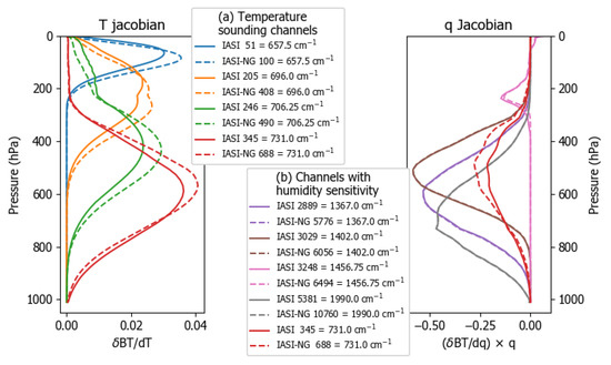
Figure 1.
Jacobians for IASI channels selected for this study (solid lines) compared with Jacobians for IASI-NG (dashed lines). A US Standard atmosphere has been used to calculate Jacobians in RTTOV, and perturbations are per layer (using 50 layers). Channel number and frequency (wavenumber) are displayed in the legend. (a) Four temperature sounding channels (Jacobian for brightness temperature BT (K) and atmospheric temperature T (K)); (b) Four humidity sounding channels in addition to one nominal temperature sounding channel at 731 cm−1 which exhibits sensitivity to humidity (Jacobian for specific humidity q (kg/kg)).
Jacobians for seven MWS temperature sounding channels and five MWS humidity sounding channels are shown in Figure 2. IASI-NG and MWS channels in our study were selected as (i) being relatively insensitive to the surface, and (ii) having Jacobians peaking within the vertical range of GRUAN sonde profiles. As for IASI-NG, we can use the GRUAN processor to map NWP-GRUAN differences into brightness temperatures at the MWS channel frequencies for the 12 selected channels.
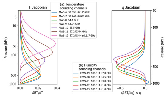
Figure 2.
Jacobians for MWS channels selected for this study. A US Standard atmosphere has been used to calculate Jacobians in RTTOV, and perturbations are per layer (using 50 layers). Channel number and frequency (GHz) are displayed in the legend. (a) Seven temperature sounding channels (Jacobian as in Figure 1); (b) Five humidity sounding channels (Jacobian ). Note the vertical scales in (a) and (b) are different.
3. Results
3.1. Calibration and Validation of Current Missions
Data sets for each instrument (Table 1) were evaluated for a common period in coordination at ECMWF and the Met Office. These periods were March-August 2015 (AMSR2); all of 2016 (MWHS-2); August-November 2016 (MWRI). For GMI three periods were selected: August–September 2016, December 2016 to January 2017, and 6 March 2017 to 20 March 2017. The latest of these periods occurred after a calibration change on 4 March 2017 affecting GMI Level 1c data. Having applied quality controls to the data sets as described in Section 2.1.3, we investigate the instrument state and geophysical state dependence of O-B differences.
In this section we present examples of O-B anomaly detection which serve to illustrate the power of the NWP framework for instrument evaluation. These comprise only part of the investigations performed for GAIA-CLIM: for a more complete overview the reader is referred to the project deliverable reports [32,33,34].
3.1.1. Detection of Geographic Biases
It can be instructive to view global maps of O-B for a few satellite orbits to see if geographic features emerge. We show mean-subtracted O-B maps over a 12-h period for MWRI in Figure 3. The maps show a clear bias difference between the ascending and descending orbits for both channels shown, for both ECMWF and Met Office statistics. Importantly, such a bias is not observed for the equivalent channels of AMSR2 and GMI, at either ECMWF or the Met Office, which gives us confidence that the bias is instrument-related. The magnitude of this bias between ascending and descending nodes is approximately 2 K (ascending minus descending) for all MWRI channels. Ascending-descending biases have been observed previously for other imagers including F-16 SSMI/S (Special Sensor Microwave - Imager/Sounder) [7]. In this case the orbital bias was diagnosed to be due to solar heating of the reflector leading to an emission which varied depending on whether the instrument was in sunlight or shade. Similar solar-dependent biases were also seen for the TMI instrument [8].
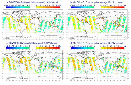
Figure 3.
Global maps of FY-3C MWRI O-B departures for a 12-h period on 15 September 2016, shown for (a) 10H channel, ECMWF statistics; (b) 10H channel, Met Office statistics; (c) 23V channel, ECMWF statistics; and (d) 23V channel, Met Office statistics. The mean global bias has been subtracted in each plot.
Recently, a physically-based correction has been developed for FY-3C MWRI to mitigate the effects of hot load reflector emission on the calibration [41]. By accounting for how the hot reflector temperature varies around the orbit due to illumination by the sun, and estimating the contribution of the hot reflector emissivity, the new algorithm results in a substantially reduced ascending–descending bias. Figure 4 compares global maps of MWRI O-B using the Met Office model for the 10.65 GHz V-polarization channel, where the original instrument calibration is compared with the revised correction [41]. A test data set for 17 August 2017 was used. The new algorithm is shown in Figure 4 to be successful in reducing the ascending–descending bias. MWRI data are currently being assimilated successfully at NWP centers such as the Met Office alongside other comparable microwave imagers.
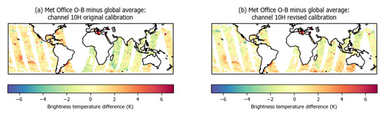
Figure 4.
Global maps of FY-3C MWRI 10.65 GHz H-polarization channel O-B departures (Met Office model) for a 10-h period on 17 August 2017, shown for (a) the original calibration algorithm; (b) with a correction [41] applied to the calibration algorithm. The mean global bias has been subtracted in each plot.
As with MWRI, we can investigate GMI O-B statistics for signs of geographic patterns such as ascending-descending differences. We focus on the period 6–20 March 2017 after the GMI calibration change. Daytime observations, defined as observations obtained between 08:00 and 15:00 local time, correspond to the descending orbit and night-time observations, defined as observations obtained between 20:00 and 03:00 local time, correspond to the ascending orbit. The mean difference ascending minus descending (or night minus day) is shown in Figure 5 for GMI imaging channels. Both ECMWF and Met Office datasets show no significant ascending/descending bias, with double differences ranging from –0.1 to 0.25 K. This is much lower than the MWRI ascending–descending departure difference of ~2 K in Figure 3, supporting GMI’s status as a calibration standard.
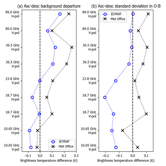
Figure 5.
(a) difference between the background departure from GMI ascending and descending nodes for the Met Office dataset (black) and ECMWF (blue) for the period 6–20 March 2017; (b) difference between the 1σ standard deviation in the ascending-descending departures.
3.1.2. Detection of Time-Dependent Biases
Accumulated statistics from NWP DA systems allow us to monitor the performance of instruments over time. We show in Figure 6 time series of mean O-B for five MWHS-2 channels, where discontinuities are observed of magnitude 0.2–0.3 K for 118 GHz channels and 2–3 K for channels 13 and 14 at 183.3 GHz. The O-B departures for the Met Office and ECMWF models are very similar, and show the same discontinuities, which suggests instrument calibration errors may be largely responsible for the biases. Figure 6 also shows how the instrument environment temperature varies with time. There is a clear correlation (or anticorrelation) between environment temperature and changes in O-B for some channels, seen most noticeably for MWHS-2 channels 13 and 14. It is unclear why changes in the instrument environment temperature should lead to changes in the MWHS-2 biases, since any changes in the systematic errors of the antennas should be removed by the calibration process. One possibility is that a change in detector non-linearity could be responsible although this awaits further investigation. Nevertheless, this finding demonstrates the ability of the NWP framework to identify sudden changes in instrument calibration. We note that the time-varying bias in MWHS-2 data has not prevented the instrument being used operationally at NWP centers, since ECMWF, the Met Office and others employ a variational bias correction scheme [42] that updates corrections to the observations every assimilation cycle.
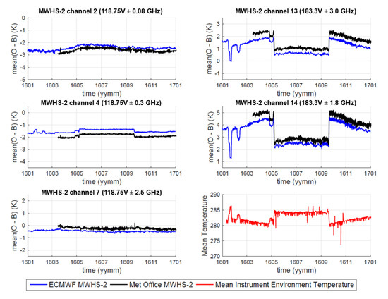
Figure 6.
The first five panels show time series of daily mean O-B for MWHS-2 channels 2, 4, 7, 13 and 14 (channel frequencies 118.75 V ± 0.08, 118.75 V ± 0.3, 118.75 V ± 2.5, 183.3 V ± 3.0 and 183.3 V ± 1.8 GHz respectively). ECMWF statistics are shown in blue, Met Office data in black for January-December 2016. The final panel shows the mean MWHS-2 instrument environment temperature as reported in direct broadcast data received by the Met Office.
3.1.3. Detection of Radio Frequency Interference
We find that global maps of O-B departures are sensitive to phenomena such as radio frequency interference (RFI) due to commercial transmissions at frequencies used by meteorological satellites. In Figure 7 we observe atypically large positive departures along the coastline of the United States for GMI channels at 18.7 GHz (we see this positive O-B anomaly for all periods studied). The coastline bias is in excess of 3 K and is spatially limited to the US territory, i.e., not extending over Canadian or Mexican coastlines. This bias can be traced back to RFI from US television providers whose satellites broadcast at frequencies between 18.3 and 18.8 GHz [43]. In comparison, the GMI RFI detection algorithm appears to perform well for the 10.65 GHz channels that are also prone to RFI by screening out affected data over Europe (not shown).
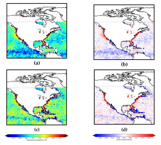
Figure 7.
Departure maps for GMI centered over North America for the period August-September 2016. All data were processed at ECMWF using the all-sky framework. (a) O-B for GMI channel 3 at 18.7 GHz V-polarization; (b) Same data as (a) presented as anomaly (O-B) – mean(O-B); (c) O-B for GMI channel 4 at 18.7 GHz H-polarization; (d) Same data as (c) presented as anomaly (O-B) – mean(O-B).
3.1.4. Inter-Satellite Comparison
We have demonstrated in preceding sections the ability to detect a number of instrument calibration anomalies within the NWP framework. Nevertheless, we need to address the limits to which the framework can be used and understand the associated uncertainties.
For example, we show in Figure 8 O-B maps generated for the same channel (10.6 GHz H-polarization) on AMSR2 and GMI for the same 24-h period. This channel was mapped in Figure 3a,b for MWRI, although in Figure 8 we have not subtracted the mean bias to aid a relative comparison. Overall, the departures do not exhibit marked geographic variations, suggesting that the NWP background fields used to compute O-B are sufficiently stable globally to enable a meaningful comparison from just 24 h of data. The NWP framework is acting as an intercalibration standard, revealing in this case that the AMSR2 channel is warmer than the RTTOV calculation by almost 4 K while the GMI channel matches the model/RTTOV calculation to within 1 K (these values are global averages).
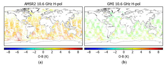
Figure 8.
Departure maps for 10.6 GHz H-polarization channels on (a) AMSR2; (b) GMI. Maps have been generated for the same period (Met Office statistics from 24 h of data on 1 July 2017).
We summarize the results of our NWP-based satellite mission assessments in Figure 9. The agreement between ECMWF and Met Office mean O-B for each instrument/channel is substantial. The two centers’ data agree that MWRI exhibits negative biases below 89 GHz for the period studied while positive biases are seen for AMSR2. For GMI the mean O-B is very small for all channels, typically less than 1 K in magnitude. As noted in Section 3.1.1, the GAIA-CLIM data analysis predates the revised calibration correction for FY-3C MWRI [41], although a negative global mean bias in O-B persists when using the updated calibration.
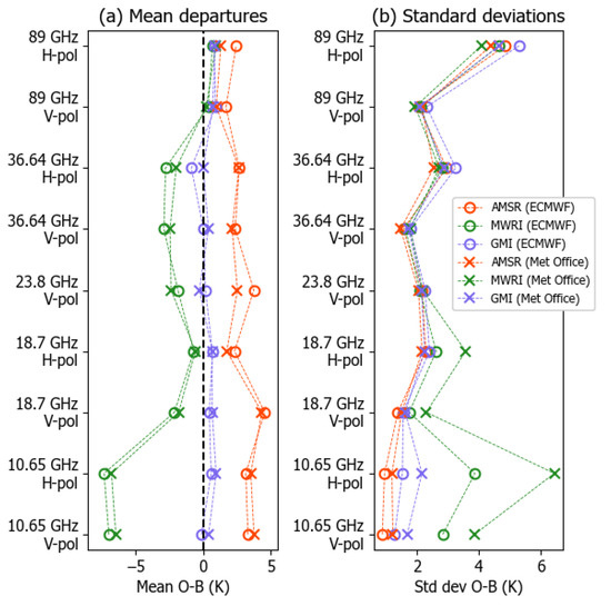
Figure 9.
A comparison of O-B statistics for common channels (vertical axis) on AMSR2 (red), MWRI (green) and GMI (blue). ECMWF data are shown as open circles, Met Office data as crosses. (a) O-B averaged globally over the data analysis periods for each instrument; (b) standard deviation in the mean O-B.
The standard deviations calculated from Met Office data tend to be larger than ECMWF for the 10.65 GHz and 18.7 GHz channels in Figure 9b. One factor affecting the statistics is proximity to the coast or small islands, since the lower frequency footprints are larger and part of the field of view can potentially be affected by land surface signals. This, along with differences in spatial thinning and averaging at ECMWF and the Met Office, likely contributes to the discrepancy in standard deviations.
The very small mean O-B biases for GMI in Figure 9 may reflect a high calibration accuracy due to improvements in the instrument design (see Section 2.1.1). However, the mean O-B can be affected by a range of other bias sources, such as errors in the radiative transfer used to translate the NWP background into a simulated radiance (especially errors in surface emissivity), or biases in the model fields (e.g. total column humidity). It is possible that radiative transfer errors or biases in the model background are compensating for GMI biases in these statistics. At the same time, the striking similarity between the O-B differences from two different NWP systems may suggest that the biases in the background values are comparatively small.
The GAIA-CLIM project identified uncertainty in surface emission as a key gap in our ability to perform cal/val studies of microwave imager missions. One of the project thematic recommendations supported improved quantification of the effects of surface properties to reduce uncertainties in satellite data assimilation, retrieval and satellite to non-satellite data comparisons. Activities are underway to establish a reference model for ocean emissivity with traceable uncertainties [44]. Recent work [45] found uncertainties in laboratory measurements of the seawater dielectric constant are in some cases inconsistent with the permittivity model used by FASTEM to calculate the ocean surface emissivity, particularly at low temperatures and below 20 GHz.
3.2. Calibration and Validation of Future Missions
We wish to evaluate the role of NWP as more than just a relative reference for satellite evaluation. To do this we need to understand uncertainties related to the accuracy of NWP temperature and humidity fields as well as uncertainties in radiative transfer and surface emission modelling. The microwave imager instruments we have considered so far exhibit high surface sensitivity such that the uncertainty related to the emissivity of the sea surface is dominant. However, for satellite temperature and humidity sounders the signal from the atmosphere dominates. Here, we consider how NWP uncertainties, traceably linked to reference GRUAN measurements, impact on the ability to characterize future missions such as the sounders MWS and IASI-NG described in Section 2.2.3.
3.2.1. IASI-NG
Using the GRUAN processor to translate NWP-GRUAN profile differences into top-of-atmosphere brightness temperatures at IASI-NG frequencies, we test the statistical significance of the differences in Figure 10 for ECMWF model fields. Depending on the channel, at least 593 GRUAN profiles were used to derive statistics. For each channel, we show the distribution of pairwise differences (as boxes and whiskers) corresponding to the left-hand side of Equation (10). The combined uncertainty estimate for NWP and GRUAN profiles (the dotted red line in Figure 10) represents the square root term on the right hand side of Equation (10). Then, for a coverage factor of k = 2, we expect 95.5% of match-ups to satisfy the inequality in Equation (10) (rewritten as Equation (12)) in order to conclude there is statistical agreement.
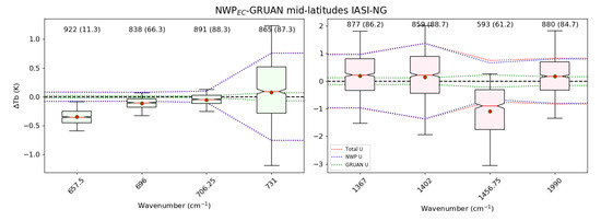
Figure 10.
Box plot summarizing ECMWF NWP-GRUAN differences for IASI-NG at mid-latitudes. The channel frequency is displayed on the horizontal axis. For each channel the mean NWP-GRUAN difference (ΔTb (K), vertical axis) is marked as a red dot; the median difference is marked as a horizontal red band at the waist of each box; the bounds of each box represent the lower and upper quartiles of the NWP-GRUAN distribution (25%–75%); the whiskers span 5%–95% of the distribution. The dotted red lines represent the total estimated uncertainty for the comparison (square root of diagonal in Equation (11) representing one standard deviation). Partial contributions to the total uncertainty are shown for the NWP model (dotted blue lines) and for GRUAN components (dotted green lines); these were calculated from the components and respectively in Equation (11). Above each box the number of profile match-ups is displayed alongside the percentage (in brackets) of match-ups in agreement following Equation (12). Temperature sounding channel boxes are shaded in green, humidity sounding channel boxes are shaded in red.
We find that none of the channel differences in Figure 10 achieve the significance threshold of 95.5%. This might suggest that the total combined uncertainty as expressed in Equation (11) is underestimated, either in terms of the component NWP and GRUAN uncertainties or due to neglected sources of uncertainty such as spatial representativeness errors. Alternatively, a lack of agreement between NWP and GRUAN profiles may result from systematic biases in NWP fields, since we account for random NWP errors only in our uncertainty estimate. We expect that a combination of random and systematic terms will contribute to the overall uncertainty.
Five of the eight channels achieve agreement between NWP and GRUAN to a confidence value of greater than 80%. The channel at 657.5 cm−1 is an outlier, with a marked negative NWP-GRUAN bias, and only 11% of match-ups are in statistical agreement according to prescribed uncertainty estimates. This channel peaks in the stratosphere (Figure 1), where there is a known systematic bias in ECMWF temperature fields [46].
Corresponding statistics for Met Office fields are shown in Figure 11. There is no stratospheric temperature bias in this case, although only one of the four temperature sounding channels (at 731 cm−1) achieves agreement to the 95% level. This is the lowest-peaking temperature channel and has significant sensitivity to humidity in the troposphere which increases the combined estimated uncertainty to 1.5 K. Statistical agreement is achieved to a level of at least 93% for all four water vapor channels, albeit with respect to relatively large combined uncertainties of between 1.2 and 2.5 K. We note that for cases where more than the expected 95% of NWP-GRUAN differences fall within expected uncertainties (for k = 2, as in Equation (12)) we should consider the possibility that the combined GRUAN and NWP uncertainties are overestimates.
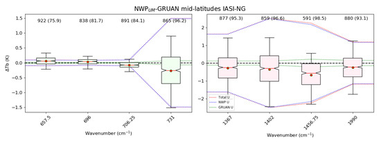
Figure 11.
As Figure 10, box plot summarizing Met Office (Unified Model) NWP-GRUAN differences for IASI-NG at mid-latitudes.
It is notable that the total uncertainty estimates in Figure 10 and Figure 11 are dominated by the NWP contribution, derived from B matrix covariances. For the three channels at 657.5, 696 and 706.25 cm−1, the uncertainty associated with NWP temperature fields is close to 0.1 K, with minimal contributions from other sources. For the other IASI-NG channels, at 731 cm−1 and larger wavenumbers, their significant humidity Jacobians result in estimated uncertainties of at least 0.75 K. This reflects the comparatively greater uncertainties in NWP humidity compared with temperature profiles.
Considering the IASI-NG channel at 706.25 cm−1 in Figure 10 and Figure 11, the mean NWP-GRUAN difference is −0.05 K (ECMWF) and −0.08 K (Met Office) with estimated total uncertainties 0.10 K and 0.10 K respectively. Neither of these comparisons reaches statistical significance to the 95.5% level, which suggests that the total uncertainty estimate for the comparison is somewhat underestimated or that a systematic bias between NWP and GRUAN profiles exists (or both). To illustrate our sensitivity to estimated uncertainty, we can scale the NWP uncertainties in an ad hoc way in order to reach the 95.5% threshold. We find that increasing the NWP uncertainty so that the total uncertainty reaches 0.13 K (ECMWF) and to 0.15 K (Met Office) achieves statistical agreement between the NWP profiles and GRUAN radiosondes. For the IASI-NG channel at 696 cm−1, the Met Office-GRUAN comparison (mean difference 0.03 K) is statistically consistent with a total uncertainty increased from 0.09 K to 0.13 K. We cannot be sure that the NWP uncertainty needs to be adjusted in this way, since other sources such as spatial representativeness errors are not included in our uncertainty budget. Nevertheless, this finding suggests the total uncertainty (dominated by NWP uncertainty, including the possibility of a small systematic bias) for these cases is unlikely to far exceed 0.15 K.
We can perform a similar exercise for a humidity sounding channel. For the IASI-NG channel at 1367 cm−1 the mean NWP-GRUAN difference is 0.20 K (ECMWF) and –0.27 K (Met Office). For the Met Office, the estimated total uncertainty for this channel is 1.63 K and already satisfies the 95% level of agreement at the k = 2 level. For ECMWF we need to inflate the total uncertainty from 0.98 K to 1.69 K to achieve statistical agreement for the comparison. For both centers’ results, across all four humidity sounding channels, we find the total uncertainty needs to be greater than 1 K to achieve statistical significance. The smallest uncertainty satisfying this requirement is for the ECMWF-GRUAN case at 1990 cm−1 where we need to increase the uncertainty from 0.83 K to 1.31 K.
It remains to consider whether, given the very stringent IASI-NG design requirement for a 0.25 K absolute calibration accuracy, a quantitative assessment of this new mission within the NWP framework is possible. While uncertainties for humidity sounding channels are too large to make meaningful statements about O-B differences at the sub-1 K level, we find that for certain temperature sounding channels (our example at 706.25 cm−1) a total uncertainty of 0.15 K is consistent with NWP-GRUAN comparisons. When investigating IASI-NG O-B statistics we would need to assess whether the differences are small enough to satisfy statistical agreement with observation and NWP uncertainties, as in Equation (10). The uncertainty in IASI-NG observations will include a random component (instrument noise, which can be reduced by taking multiple measurements as in Equation (8)) and a systematic component accounting for the expected calibration accuracy. It is difficult to estimate and partition the relative contributions of random and systematic uncertainties related to NWP fields. We would also need to account for additional sources of uncertainty, for example due to possible errors in radiative transfer calculations. It is therefore not certain that a uniform bias of 0.25 K could be detected from O-B, although calibration errors giving rise to geographical patterns in O-B biases, as in Figure 3, would be more easily detected.
3.2.2. MWS
NWP-GRUAN differences, translated to top-of-atmosphere brightness temperature for MWS channels, are summarized for ECMWF fields in Figure 12 and Met Office fields in Figure 13. Once again, the temperature sounding channels peaking in the stratosphere exhibit a negative bias for the ECMWF comparison. For the two lowest-peaking temperature channels (MWS channels 6 and 7 at 53.60 ± 0.115 GHz and 53.95 ± 0.081 GHz respectively) agreement is achieved with a confidence interval of 97% or greater, for both ECMWF and the Met Office. However, for the remaining temperature channels agreement to within 95% is not reached. Interestingly, for MWS channels 6 and 7, the largest contribution to the NWP uncertainty stems from the surface contribution. This motivates future work exploring whether the component uncertainty estimates need to be revised.
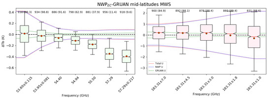
Figure 12.
As Figure 10, box plot summarizing ECMWF NWP-GRUAN differences for MWS at mid-latitudes.
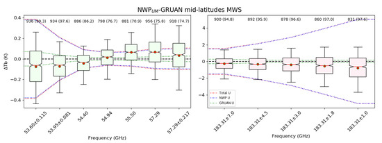
Figure 13.
As Figure 10, box plot summarizing Met Office NWP-GRUAN differences for MWS at mid-latitudes.
Considering the five MWS humidity channels, agreement of GRUAN profiles with ECMWF fields is achieved in Figure 12 with a confidence interval in the range 85–89%, depending on the channel, i.e., somewhat below the 95.5% level of statistical consistency expected for a coverage factor k = 2 [36]. For Met Office fields in Figure 13 agreement is reached at the 95%–98% level. Taken at face value, these results would suggest that the overall uncertainty for the comparisons (dominated for 183 GHz channels by NWP B matrix humidity uncertainty) is estimated too small in the ECMWF case and a little too large in the Met Office case. However, this should not disguise the qualitative agreement between estimated uncertainties and spread of NWP-GRUAN differences for both centers’ results.
As noted in Section 2.2.3, the MWS design requirement is for an absolute radiometric bias of less than 1 K for all channels. This is greater than the 0.2–0.4 K combined uncertainties for the two temperature sounding channels in Figure 12 and Figure 13 where there is statistical agreement at (greater than) the 95.5% level. We can conclude a radiometric bias of 1 K for an MWS-like temperature sounding channel is detectable in current NWP frameworks.
We have drawn conclusions for MWS and IASI-NG based on statistics for mid-latitude GRUAN profiles. However, for sub-tropical GRUAN sites we see less consistency (not shown) between NWP and GRUAN for both ECMWF and the Met Office, albeit with fewer collocations over the period to assess. The greater water vapor burden in tropical atmospheres raises the peak height of humidity Jacobians compared with higher latitudes, which changes the overall uncertainty estimates. It is also likely that model biases vary between different regions. For northern latitudes, the distribution of NWP-GRUAN differences is broadly similar to that at mid-latitudes. However, for MWS humidity channels, there is greater sensitivity to the surface at high latitudes. This applies especially to MWS channel 19 at 183.3 ± 7.0 GHz where the surface contribution dominates the uncertainty for both GRUAN and NWP components.
We can attempt to quantify the overall level of agreement between NWP fields and GRUAN profiles by applying the test as in Equation (13). The test does not reach the 95.5% level for MWS or IASI-NG, for either ECMWF or Met Office comparisons. This is suggestive that the uncertainty has been under-represented in as expressed in Equation (11). However, there are some marked latitudinal variations in the statistics, with results in the range 82%–89% at northern latitudes but only 62%–72% in the sub-tropics. This may indicate that the use of global-average NWP B matrices does not capture important aspects of uncertainties in NWP fields, particularly geographic variations. It might be possible to improve on the representation of NWP uncertainty, for example sampling B separately for each geographic area of interest, but this is beyond the scope of the current work.
4. Discussion
In this paper we have presented examples of satellite validation studies within the NWP framework. The advantages of evaluating instrument performance with O-B statistics is apparent for the case of MWRI ascending/descending biases in Section 3.1.1, highlighting the ability to perform a comprehensive global validation with 12 h of data. While there will continue to be an essential role for dedicated efforts such as field campaigns, which offer high quality though sparse validation data sets, the NWP framework is increasingly being used as a powerful tool for cal/val activities.
The summary of AMSR2, MWRI and GMI O-B statistics in Figure 9 serves to illustrate the value of NWP as a comparative reference, revealing inter-sensor brightness temperature differences of several K. For GMI the O-B bias is within ±1 K for all channels, consistent with its status as a calibration standard. Statistics are very similar for both ECMWF and the Met Office, which gives us confidence that inter-model differences are not critical for studies of this kind. However, we acknowledge that there remain gaps in our ability to perform quantitative assessments, particularly for microwave imagers which exhibit high sensitivity to the surface. We do not currently have robust estimates of the uncertainty that results from using sea surface emission models such as FASTEM. Advances have been made recently in characterizing the uncertainty in the permittivity component of this model [45] but more efforts are needed.
The GRUAN processor allows us to test the statistical significance of differences between NWP and sonde profiles when transformed into observation space. We expect 95.5% of pairwise differences to fall within the k = 2 bound in Equation (10) if, crucially, we have estimated GRUAN and NWP uncertainties correctly and if the NWP model is not affected by systematic biases. We can think of the comparison, therefore, as a consistency check on the specified uncertainties.
For some, though not all, of the comparisons shown in Figure 10, Figure 11, Figure 12 and Figure 13, fewer than the expected number of NWP-GRUAN differences lie within expected bounds. There are a number of possible reasons for this. Firstly, we do not account for systematic NWP model biases in our formulation of the uncertainty in Equation (11) since the B matrix only represents randomly distributed errors. It is therefore not surprising that the GRUAN profiles and ECMWF NWP equivalents proved to be significantly different for high-peaking temperature sounding channels, since we are confirming a known stratospheric temperature cold model bias. Our results show that GRUAN uncertainties are sufficiently constrained to allow a model bias of up to 0.5 K [46] to be detectable in our framework. In principle, the reduced test (Equation (13)) removes a dependence on the mean bias. However, the application of Equation (13) still relies on appropriately estimated random uncertainties.
Secondly, our uncertainty formulation neglects the role of spatial representativeness errors. We are comparing NWP profiles characterized by a spatial resolution of approximately 10 km with radiosonde measurements which capture atmospheric profiles at very fine scales. This inevitable scale mismatch introduces an additional uncertainty in the comparison (only vertical interpolation uncertainty is accounted for in Equation (11)). However, we expect scale mismatch to contribute to the spread of the NWP-GRUAN distribution without necessarily affecting the mean difference significantly. Attempts to estimate the magnitude of spatial representativeness errors will rely on future work.
Thirdly, we are sensitive to possible over- or under-estimates of NWP uncertainty represented by the B matrix, which includes covariances for temperature and humidity profiles (as well as surface variables calculated from the variance of model surface parameters at each launch site). This may explain differences in NWP-GRUAN statistics between geographic zones, with greater surface sensitivity at high latitudes and a larger impact due to water vapor in the sub-tropics. In this work we have used global-mean B matrices; it might be possible to improve on our method by using B matrices representing “errors of the day” at a particular location and date.
Fourthly, our specification of the GRUAN uncertainty matrix (R in Equation (11)) is sub-optimal. We lack information about how uncertainties are correlated between vertical levels, so we use a diagonal R matrix with off-diagonal covariances of zero. Further, the GRUAN total uncertainty at each level comprises both systematic and random uncertainties combined in quadrature. We note, though, that for most of the cases we have considered estimates of NWP uncertainty far exceeded those attributed to GRUAN radiosondes.
For channels sensitive to water vapor, estimated combined uncertainties for the NWP-GRUAN comparison are typically 1–3 K. Agreement for most of these channels is achieved at a confidence level of 85% or more, which suggests these uncertainties are not wholly unrealistic. As a result, we are not able to validate NWP humidity fields to any better than 1 K in terms of sensor brightness temperature. The lower confidence level in sub-tropical NWP-GRUAN comparisons needs further investigation.
Conversely, for most temperature sounding channels we find combined uncertainties for NWP-GRUAN comparisons in the range 0.1–0.4 K, achieving statistical agreement at the 99% level for two of the MWS channels in this study. As a sensitivity study, we have also tried inflating the NWP component of the total uncertainty in order to bring the expected 95.5% of match-up differences within the k = 2 uncertainty bound (Equation 12). For the 706.25 cm−1 IASI-NG temperature sounding channel a total uncertainty of 0.13–0.15 K is sufficient to achieve statistical significance. We use this value as a reasonable estimate for the total NWP-GRUAN uncertainty that is consistent with the distribution of NWP-GRUAN differences, while acknowledging that more work needs to be done to finesse estimates of uncertainty in Equation (11).
The uncertainty estimates we use are valid for assessing the statistical agreement between NWP-GRUAN profiles for a set of collocations. Estimating the uncertainty in the mean NWP-GRUAN difference for each instrument channel is more difficult. To do this, we would need to know whether NWP and GRUAN uncertainties are systematic and correlated between match-ups (limiting case in Equation (9)) or whether the uncertainties are partly random in character and can be reduced by averaging a large number of match-ups (limiting case in Equation (8)). In reality, both NWP fields and GRUAN profiles are likely to exhibit a combination of random and systematic uncertainties. Since our knowledge is incomplete, a conservative assumption is that the mean pairwise uncertainties are correlated and irreducible by averaging. This is likely to err on the pessimistic side when assigning uncertainty bounds to the mean differences.
The data assimilation and observation processing systems at NWP centers undergo regular upgrades. We expect, therefore, that the accuracy and bias characteristics of NWP fields will change over time. In our study, the NWP-GRUAN comparison provides a snapshot of model uncertainty evaluation from 2016. The GRUAN processor provides us with the means of tracking changes in the quality of NWP outputs over time.
We note the NWP and GRUAN collocated profiles, when converted to top-of-atmosphere brightness temperatures, use a common operator (RTTOV). Thus, any uncertainties in RTTOV itself (for example due to limitations in our knowledge of spectroscopy) cancel and are not included in the uncertainty for the comparison. A complete closure of the uncertainty budget for NWP-based assessments of new satellite missions using O-B statistics, however, will need to take estimated radiative transfer errors into account, in addition to the spatial representativeness uncertainties that result from scale mismatch between satellite footprints and the NWP model grid.
5. Conclusions
The European Union GAIA-CLIM project examined the calibration/validation of Earth observation data sets using non-satellite reference data. We have explored the role of NWP frameworks for assessing the data quality of recent satellite missions at two centers, ECMWF and the Met Office. As a demonstration of the utility of NWP systems for characterizing satellite measurements, we show examples in this paper of anomaly detection such as identifying geographically- and temporally-varying calibration biases and radio frequency interference. We also acknowledge limitations in the use of NWP for validation, particularly uncertainties in surface emission which remain poorly constrained. This means that while we can identify inter-satellite biases for surface-sensitive channels on microwave imagers (at frequencies typically below 89 GHz) it is difficult to assign an absolute uncertainty to differences between observed radiances and NWP model equivalents.
We have attempted to make an improved assessment of uncertainties for NWP fields by comparison with GRUAN reference radiosondes. In terms of top-of-atmosphere brightness temperature, for selected temperature sounding channel frequencies, we find NWP-GRUAN differences are in statistical agreement within an estimated combined uncertainty of 0.15 K. In contrast, for humidity sounding channels, the combined uncertainty is generally greater than 1 K. In both cases the NWP model uncertainty is the dominant contribution. We conclude that, given the relative accuracy of NWP temperature compared with humidity fields or surface variables, the validation of new instruments is most easily pursued by examining temperature sounding channels with minimal surface sensitivity.
The prospects for the NWP validation of future sounding missions have been considered. For the IASI-NG hyperspectral infrared sounder, with a stringent design requirement for radiometric calibration accuracy of 0.25 K, validation within the NWP framework tests the limits of current capabilities. Conversely, any biases exceeding the radiometric bias requirement of 1 K for the MWS microwave sounder temperature channels should be straightforwardly detectable using NWP fields as a reference.
Author Contributions
Conceptualization, W.B. and S.N.; methodology, S.N., F.C., H.L. and W.B.; software, S.N., F.C. and H.L.; validation, S.N., F.C. and H.L.; formal analysis, S.N., F.C. and H.L.; investigation, S.N., F.C. and H.L.; resources, S.N., F.C., H.L. and K.S.; data curation, S.N., F.C., H.L. and K.S.; writing—original draft preparation, S.N. and F.C.; writing—review and editing, S.N., F.C., H.L., N.B. and K.S.; visualization, S.N., F.C. and H.L.; supervision, W.B., N.B. and S.N.; project administration, W.B., N.B. and S.N.; funding acquisition, W.B. All authors have read and agreed to the published version of the manuscript.
Funding
The work presented in this report was funded by the European Union’s Horizon 2020 research and innovation program under the GAIA-CLIM project (grant agreement No. 640276).
Acknowledgments
We thank colleagues at ECMWF (Stephen English, Bruce Ingleby, Peter Lean, Jacqueline Farnan and Alan Geer) and the Met Office (Stefano Migliorini and Nigel Atkinson) for their assistance and useful discussions during the project. We are grateful to Qifeng Lu (National Satellite Meteorological Center, China Meteorological Administration) for providing test data for FY-3C MWRI.
Conflicts of Interest
The authors declare no conflict of interest.
References
- Loew, A.; Bell, W.; Brocca, L.; Bulgin, C.E.; Burdanowitz, J.; Calbet, X.; Donner, R.V.; Ghent, D.; Gruber, A.; Kaminski, T.; et al. Validation practices for satellite-based Earth observation data across communities. Rev. Geophys. 2017, 55, 779–817. [Google Scholar] [CrossRef]
- Newman, S.M.; Knuteson, R.O.; Zhou, D.K.; Larar, A.M.; Smith, W.L.; Taylor, J.P. Radiative transfer validation study from the European Aqua Thermodynamic Experiment. Q. J. R. Meteorol. Soc. 2009, 135, 277–290. [Google Scholar] [CrossRef]
- Larar, A.M.; Smith, W.L.; Zhou, D.K.; Liu, X.; Revercomb, H.; Taylor, J.P.; Newman, S.M.; Schlüssel, P. IASI spectral radiance validation inter-comparisons: Case study assessment from the JAIVEx field campaign. Atmos. Chem. Phys. 2010, 10, 411–430. [Google Scholar] [CrossRef]
- Müller, R. Calibration and Verification of Remote Sensing Instruments and Observations. Remote Sens. 2014, 6, 5692–5695. [Google Scholar] [CrossRef]
- Cao, C.Y.; Weinreb, M.; Xu, H. Predicting simultaneous nadir overpasses among polar-orbiting meteorological satellites for the intersatellite calibration of radiometers. J. Atmos. Ocean. Technol. 2004, 21, 537–542. [Google Scholar] [CrossRef]
- Wang, L.K.; Goldberg, M.; Wu, X.Q.; Cao, C.Y.; Iacovazzi, R.A.; Yu, F.F.; Li, Y.P. Consistency assessment of Atmospheric Infrared Sounder and Infrared Atmospheric Sounding Interferometer radiances: Double differences versus simultaneous nadir overpasses. J. Geophys. Res. Atmos. 2011, 116, 11. [Google Scholar] [CrossRef]
- Bell, W.; English, S.J.; Candy, B.; Atkinson, N.; Hilton, F.; Baker, N.; Swadley, S.D.; Campbell, W.F.; Bormann, N.; Kelly, G.; et al. The assimilation of SSMIS radiances in numerical weather prediction models. IEEE Trans. Geosci. Remote Sens. 2008, 46, 884–900. [Google Scholar] [CrossRef]
- Geer, A.J.; Bauer, P.; Bormann, N. Solar Biases in Microwave Imager Observations Assimilated at ECMWF. IEEE Trans. Geosci. Remote Sens. 2010, 48, 2660–2669. [Google Scholar] [CrossRef]
- Lu, Q.F.; Bell, W.; Bauer, P.; Bormann, N.; Peubey, C. Characterizing the FY-3A Microwave Temperature Sounder Using the ECMWF Model. J. Atmos. Ocean. Technol. 2011, 28, 1373–1389. [Google Scholar] [CrossRef]
- Saunders, R.W.; Blackmore, T.A.; Candy, B.; Francis, P.N.; Hewison, T.J. Monitoring Satellite Radiance Biases Using NWP Models. IEEE Trans. Geosci. Remote Sens. 2013, 51, 1124–1138. [Google Scholar] [CrossRef]
- Lu, Q.F.; Bell, W. Characterizing Channel Center Frequencies in AMSU-A and MSU Microwave Sounding Instruments. J. Atmos. Ocean. Technol. 2014, 31, 1713–1732. [Google Scholar] [CrossRef][Green Version]
- Carminati, F.; Migliorini, S.; Ingleby, B.; Bell, W.; Lawrence, H.; Newman, S.; Hocking, J.; Smith, A. Using reference radiosondes to characterise NWP model uncertainty for improved satellite calibration and validation. Atmos. Meas. Technol. 2019, 12, 83–106. [Google Scholar] [CrossRef]
- Saunders, R.; Hocking, J.; Turner, E.; Rayer, P.; Rundle, D.; Brunel, P.; Vidot, J.; Roquet, P.; Matricardi, M.; Geer, A.; et al. An update on the RTTOV fast radiative transfer model (currently at version 12). Geosci. Model Dev. 2018, 11, 2717–2732. [Google Scholar] [CrossRef]
- Rabier, F.; Jarvinen, H.; Klinker, E.; Mahfouf, J.F.; Simmons, A. The ECMWF operational implementation of four-dimensional variational assimilation. I: Experimental results with simplified physics. Q. J. R. Meteorol. Soc. 2000, 126, 1143–1170. [Google Scholar] [CrossRef]
- Rawlins, F.; Ballard, S.P.; Bovis, K.J.; Clayton, A.M.; Li, D.; Inverarity, G.W.; Lorenc, A.C.; Payne, T.J. The Met Office global four-dimensional variational data assimilation scheme. Q. J. R. Meteorol. Soc. 2007, 133, 347–362. [Google Scholar] [CrossRef]
- English, S.J.; Renshaw, R.J.; Dibben, P.C.; Smith, A.J.; Rayer, P.J.; Poulsen, C.; Saunders, F.W.; Eyre, J.R. A comparison of the impact of TOVS and ATOVS satellite sounding data on the accuracy of numerical weather forecasts. Q. J. R. Meteorol. Soc. 2000, 126, 2911–2931. [Google Scholar]
- Imaoka, K.; Kachi, M.; Kasahara, M.; Ito, N.; Nakagawa, K.; Oki, T. Instrument performance and calibration of AMSR-E and AMSR2. Netw. World Remote Sens. 2010, 38, 13–16. [Google Scholar]
- Yang, H.; Weng, F.Z.; Lv, L.Q.; Lu, N.M.; Liu, G.F.; Bai, M.; Qian, Q.Y.; He, J.K.; Xu, H.X. The FengYun-3 Microwave Radiation Imager On-Orbit Verification. IEEE Trans. Geosci. Remote Sens. 2011, 49, 4552–4560. [Google Scholar] [CrossRef]
- He, J.Y.; Zhang, S.W.; Wang, Z.Z. Advanced Microwave Atmospheric Sounder (AMAS) Channel Specifications and T/V Calibration Results on FY-3C Satellite. IEEE Trans. Geosci. Remote Sens. 2015, 53, 481–493. [Google Scholar] [CrossRef]
- Draper, D.W.; Newell, D.A.; Wentz, F.J.; Krimchansky, S.; Skofronick-Jackson, G.M. The Global Precipitation Measurement (GPM) Microwave Imager (GMI): Instrument Overview and Early On-Orbit Performance. IEEE J. Sel. Top. Appl. Earth Obs. Remote Sens. 2015, 8, 3452–3462. [Google Scholar] [CrossRef]
- Draper, D.W.; Newell, D.A.; McKague, D.S.; Piepmeier, J.R. Assessing Calibration Stability Using the Global Precipitation Measurement (GPM) Microwave Imager (GMI) Noise Diodes. IEEE J. Sel. Top. Appl. Earth Obs. Remote Sens. 2015, 8, 4239–4247. [Google Scholar] [CrossRef]
- Wentz, F.J.; Draper, D. On-Orbit Absolute Calibration of the Global Precipitation Measurement Microwave Imager. J. Atmos. Ocean. Technol. 2016, 33, 1393–1412. [Google Scholar] [CrossRef]
- Bauer, P.; Geer, A.J.; Lopez, P.; Salmond, D. Direct 4D-Var assimilation of all-sky radiances. Part I: Implementation. Q. J. R. Meteorol. Soc. 2010, 136, 1868–1885. [Google Scholar] [CrossRef]
- Geer, A.J.; Bauer, P.; Lopez, P. Direct 4D-Var assimilation of all-sky radiances. Part II: Assessment. Q. J. R. Meteorol. Soc. 2010, 136, 1886–1905. [Google Scholar] [CrossRef]
- Bauer, P.; Moreau, E.; Chevallier, F.; O’Keeffe, U. Multiple-scattering microwave radiative transfer for data assimilation applications. Q. J. R. Meteorol. Soc. 2006, 132, 1259–1281. [Google Scholar] [CrossRef]
- Liu, Q.H.; Weng, F.Z.; English, S.J. An Improved Fast Microwave Water Emissivity Model. IEEE Trans. Geosci. Remote Sens. 2011, 49, 1238–1250. [Google Scholar] [CrossRef]
- Kazumori, M.; English, S.J. Use of the ocean surface wind direction signal in microwave radiance assimilation. Q. J. R. Meteorol. Soc. 2015, 141, 1354–1375. [Google Scholar] [CrossRef]
- Geer, A.J.; Bauer, P. Observation errors in all-sky data assimilation. Q. J. R. Meteorol. Soc. 2011, 137, 2024–2037. [Google Scholar] [CrossRef]
- Petty, G.W.; Katsaros, K.B. Precipitation observed over the South China Sea by the Nimbus-7 Scanning Multichannel Microwave Radiometer during winter MONEX. J. Appl. Meteorol. 1990, 29, 273–287. [Google Scholar] [CrossRef]
- Petty, G.W. Physical retrievals of over-ocean rain rate from multichannel microwave imagery .1. Theoretical characteristics of normalized polarization and scattering indexes. Meteorol. Atmos. Phys. 1994, 54, 79–99. [Google Scholar] [CrossRef]
- Lonitz, K.; Geer, A. New Screening of Cold-Air Outbreak Regions Used in 4D-Var All-Sky Assimilation. EUMETSAT/ECMWF Fellowship Programme Research Report No. 35. 2015. Available online: https://www.ecmwf.int/node/10777 (accessed on 11 May 2020).
- Newman, S.; Bell, W.; Salonen, K. Calibration/Validation Study of AMSR2 on GCOM-W1. GAIA-CLIM Deliverable Report D4.2. 2015. Available online: http://www.gaia-clim.eu/system/files/workpkg_files/D4.2_Individual%20reports%20on%20validation%20of%20satellites%20v1.pdf (accessed on 11 May 2020).
- Lawrence, H.; Carminati, F.; Bell, W.; Bormann, N.; Newman, S.; Atkinson, N.; Geer, A.; Migliorini, S. An Evaluation of FY-3C MWRI and Assessment of the Long-Term Quality of FY-3C MWHS-2 at ECMWF and the Met Office. GAIA-CLIM Deliverable Report D4.5. 2017. Available online: http://www.gaia-clim.eu/system/files/document/D4.5%20Individual%20Reports%20on%20validation%20of%20satellites%20V2.pdf (accessed on 11 May 2020).
- Lawrence, H.; Carminati, F.; Goddard, J.; Newman, S.; Bell, W.; Bormann, N.; English, S.; Atkinson, N. Individual Reports on Validation of Satellites, Version 3. GAIA-CLIM Deliverable Report D4.6. 2017. Available online: http://www.gaia-clim.eu/system/files/document/d4.6.pdf (accessed on 11 May 2020).
- Dirksen, R.J.; Sommer, M.; Immler, F.J.; Hurst, D.F.; Kivi, R.; Vomel, H. Reference quality upper-air measurements: GRUAN data processing for the Vaisala RS92 radiosonde. Atmos. Meas. Technol. 2014, 7, 4463–4490. [Google Scholar] [CrossRef]
- Immler, F.J.; Dykema, J.; Gardiner, T.; Whiteman, D.N.; Thorne, P.W.; Vomel, H. Reference Quality Upper-Air Measurements: Guidance for developing GRUAN data products. Atmos. Meas. Technol. 2010, 3, 1217–1231. [Google Scholar] [CrossRef]
- Holmlund, K.; Bojkov, B.; Klaes, D.; Schlussel, P. IEEE. The Joint Polar System: Towards the Second Generation EUMETSAT Polar System. 2017 IEEE Int. Geosci. Remote Sens. Symp. (Igarss) 2017, 2779–2782. [Google Scholar] [CrossRef]
- Schlüssel, P.; Kayal, G. Introduction to the Next Generation EUMETSAT Polar System (EPS-SG) Observation Missions. In Proceedings of the Conference on Sensors, Systems, and Next-Generation Satellites XXI, Warsaw, Poland, 11–14 September 2017. [Google Scholar]
- D’Addio, S.; Kangas, V.; Klein, U.; Loiselet, M.; Mason, G. IEEE. The Microwave Radiometers on-board MetOp Second Generation satellites. 2014 IEEE Int. Workshop Metrol. Aerosp. (Metroaerospace) 2014, 599–604. [Google Scholar] [CrossRef]
- Bermudo, F.; Rousseau, S.; Pequignot, E.; Bernard, F. IEEE. IASI-NG program: A New Generation of Infrared Atmospheric Sounding Interferometer. 2014 IEEE Int. Geosci. Remote Sens. Symp. (Igarss) 2014, 1373–1376. [Google Scholar] [CrossRef]
- Xie, X.X.; Wu, S.L.; Xu, H.X.; Yu, W.M.; He, J.K.; Gu, S.Y. Ascending-Descending Bias Correction of Microwave Radiation Imager on Board FengYun-3C. IEEE Trans. Geosci. Remote Sens. 2019, 57, 3126–3134. [Google Scholar] [CrossRef]
- Auligne, T.; McNally, A.P.; Dee, D.P. Adaptive bias correction for satellite data in a numerical weather prediction system. Q. J. R. Meteorol. Soc. 2007, 133, 631–642. [Google Scholar] [CrossRef]
- Zou, X.L.; Tian, X.X.; Weng, F.Z. Detection of Television Frequency Interference with Satellite Microwave Imager Observations over Oceans. J. Atmos. Ocean. Technol. 2014, 31, 2759–2776. [Google Scholar] [CrossRef]
- English, S.; Geer, A.; Lawrence, H.; Meunier, L.-F.; Prigent, C.; Kilic, L.; Johnson, B.; Chen, M.; Bell, W.; Newman, S. A reference model for ocean surface emissivity and backscatter from the microwave to the infrared. In Proceedings of the 21st International TOVS Study Conference, Darmstadt, Germany, 29 November–5 December 2017. [Google Scholar]
- Lawrence, H.; Bormann, N.; English, S.J. Uncertainties in the permittivity model for seawater in FASTEM and implications for the calibration/validation of microwave imagers. J. Quant. Spectrosc. Radiat. Transf. 2020, 243. [Google Scholar] [CrossRef]
- Shepherd, T.G.; Polichtchouk, I.; Hogan, R.J.; Simmons, A.J. Report on Stratosphere Task Force, ECMWF Technical Memorandum 824. 2018. Available online: https://www.ecmwf.int/en/elibrary/18259-report-stratosphere-task-force (accessed on 11 May 2020).


© 2020 by the authors. Licensee MDPI, Basel, Switzerland. This article is an open access article distributed under the terms and conditions of the Creative Commons Attribution (CC BY) license (http://creativecommons.org/licenses/by/4.0/).