Article

Assimilating SMOS Brightness Temperature for Hydrologic Model Parameters and Soil Moisture Estimation with an Immune Evolutionary Strategy

1
School of Earth Sciences and Engineering, Hohai University, Nanjing 211100, China
2
Geomatics Center of Huzhou, Huzhou 313000, China
3
College of Hydrology and Water Resources, Hohai University, Nanjing 210098, China
4
QiuZhen College, Huzhou University, Huzhou 313000, China
5
Zhejiang Province Key Laboratory of Smart Management & Application of Modern Agricultural Resources, Huzhou University, Huzhou 313000, China
*
Author to whom correspondence should be addressed.
Remote Sens. 2020, 12(10), 1556; https://doi.org/10.3390/rs12101556
Submission received: 8 April 2020 / Revised: 28 April 2020 / Accepted: 11 May 2020 / Published: 14 May 2020
(This article belongs to the Special Issue Microwave Remote Sensing for Hydrology)

Abstract

:
Hydrological models play an essential role in data assimilation (DA) systems. However, it is a challenging task to acquire the distributed hydrological model parameters that affect the accuracy of the simulations at a grid scale. Remote sensing data provide an ideal observation for DA to estimate parameters and state variables. In this study, a special assimilation scheme was proposed to jointly estimate parameters and soil moisture (SM) by assimilating brightness temperature (TB) from the Soil Moisture and Ocean Salinity (SMOS) mission. Variable infiltration capacity (VIC) hydrological model and L-band microwave emission of the biosphere model (L-MEB) are coupled as model and observation operators, respectively. The scheme combines two stages of estimators, one for the static model parameters and the other for the dynamic state variables. The estimators approximate the posterior probability distribution of an unknown target through sequential Monte Carlo (SMC) sampling. Markov chain Monte Carlo (MCMC) and immune evolution strategy are embedded in both stages to solve particle impoverishment problems. To evaluate the effectiveness of the scheme, the estimated SM sets are compared with in-situ observations and SMOS products in Maqu on the Tibetan Plateau. Specifically, the root mean square error decreased from 0.126 to 0.087 m3m−3 for surface SM, with a slight impact on the root zone. The temporal correlation between DA results and in-situ measurements increased to 0.808 and 0.755 for surface SM (+0.057) and root zone SM (+0.040), respectively. The results demonstrate that assimilating TB has tremendous potential as an approach to improve the estimation of distributed model parameters and SMs of surface and root zone at a grid scale, and the immune evolution strategy is effective for increasing the accuracy of approximation in sampling.

Graphical Abstract

1. Introduction

Soil moisture (SM) plays a fundamental role in the global energy and water cycle. It governs the partitioning of the mass and energy fluxes between the land and the atmosphere [1,2]. Therefore, accurate and reliable SM profiles are crucial in various applications, such as flood and drought monitoring, water resource management, land–atmosphere interaction studies, and even economic and policy analysis [3,4]. Generally, modeling and observation are two typical approaches to obtain SM information. According to the means of acquisition, observation can be divided into ground-based measurements and remote sensing observations. However, different approaches have their respective advantages and drawbacks.The drawbacks limit their practical applications, such as potential the bias of modeling, limited coverage of regions for ground-based measurements, and limited penetration depth of microwaves. Data assimilation (DA), merging observed data into a model, is a widely used technique to obtain continuous spatio-temporal SM in hydrology and meteorology [5,6,7].
Currently, the most common method to estimate SM is the assimilation of microwave remote sensing observations into the land surface model (LSM) and evaluation of the assimilation results using ground-based measurements [8,9,10]. With the development of satellite-based microwave missions, including the Advanced Microwave Scanning Radiometer-Earth Observing System (AMSR-E), the Soil Moisture and Ocean Salinity (SMOS) mission, and the Soil Moisture Active Passive (SMAP) mission [11], much research about SM estimation has been successfully conducted to assimilate microwave data sets, such as SM retrievals and brightness temperature (TB) [1,12,13]. Originally, SM retrievals were more widely applied to assimilation [10,14]. However, there is an increasing trend whereby TB observations are directly assimilated into LSMs [1,12,15]. LSMs and the radiative transfer model (RTM) have consistent parameters and auxiliary inputs to avoid cross-correlated errors through directly assimilating TB [15].
The performance of assimilation is mainly determined by the quality of observation, accuracy of modeling, and effectiveness of the assimilation algorithm. Thus, it is necessary to improve the simulation accuracy of a model before assimilating observations into a model. The simulation and forecasting accuracy of a model mainly depend on the quality of the model parameters, which are classified as physical parameters and process parameters. Unlike the physical parameters that can be measured directly, the process parameters mostly must be estimated (calibrated) [16]. Considering the spatio-temporal heterogeneity, a single set of parameters estimated by in-situ observations at point scale or streamflow at catchment scale may cause unrealistic spatio-temporal variability of SM. Satellite-based observations with regional and global coverage can be applied for model parameters and state variables estimation at a grid scale, which is usually larger than 10km × 10km. For instance, Yang et al. used AMSR-E TB to calibrate LSM at a grid scale [17]. Chen et al. improved SM estimation by jointly assimilation AMSR-E TB and MODIS LST products [18]. Many parameters represent conceptual or effective properties of a landscape in LSM. Usually, they are assumed to be time-invariant (static) for convenience in the hydrological literature [17,19,20,21]. Two common approaches have been proposed to estimate unknown static parameters based on sequential Monte Carlo (SMC) sampling. (1) State augmentation method. The state vector is extended with any unknown static parameter in the model. Then, DA techniques are used to track and predict the extended state vector. In fact, this method treats static parameters as time-varying and transfers parameter estimation to the filtering process [19,22,23]. (2) Geometric bridge method. The target distribution is inferred by moving smoothly from a tractable initial distribution through intermediary distribution in a sequence form based on all observations [20,24,25,26].
Different classes of DA algorithms have been successfully applied in DA applications. The ensemble Kalman filter (EnKF) and particle filtering (PF) are the most popular nonlinear filters in sequential DA. Currently, EnKF is widely used in various applications due to its computational efficiency and ease of use [10,27,28]. However, the Gaussian error assumption and linear updating rule limit the superiority of EnKF [14,29]. The PFs are also widely employed in parameters or states estimation in nonlinear LSMs [22,30,31]. One of the major advantages of PFs is that error distributions no longer need to be Gaussian. However, the filtering technology based on SMC sampling suffers from a serious problem, which is a well-known issue of particle impoverishment. This phenomenon is characterized by most particles having identical value and so the process cannot sufficiently approximate the posterior distribution, which leads to inaccurate estimations. Particles usually need to be estimated by Markov chain Monte Carlo (MCMC) method to mitigate the impoverishment problem [32,33].
In addition, evolutionary computation methods have also been embedded into the assimilation framework for their well-known global search ability to improve the quality and diversity of particles. Vrugt et al. proposed Particle-DREAM, combining the strengths of SMC, MCMC, and differential evolution (DE) algorithm for hydrologic DA [19]. Abbaszadeh et al. designed an improved PF algorithm with genetic algorithm (GA) and MCMC simulation to enhance the hydrologic forecast [23]. Zhu et al. presented a new moving strategy incorporating GA, DE, and MCMC for optimizing the hydrologic model [20]. Among these intelligent optimization and search methods, the Particle-DREAM algorithm is widely applied in numerous practical applications and has proven its effectiveness. In addition, Ju et al. proposed an immune evolution PF inspired by the biological immune system for SM estimation [34]. The mechanism of antibody diversity preservation and immune memory function are imitated to generate candidate particles with more prior information for the MCMC step and ensure particle evolution towards optimal estimation. The immune evolution strategy has been successfully applied in DA and verified by highly the nonlinear and high-dimensional Lorenz96 atmospheric model, which is usually performed as a benchmark to validate DA algorithms [35,36], and the variable infiltration capacity (VIC) model through ground-based measurements. Compared with Particle-DREAM and EnKF, the immune evolution PF consistently receives the best performance in both synthetic experiments and real cases. A major limitation of immune evolution PF is the higher computational cost when ensemble size is larger than 100 (for more detail, see [34]). However, these works mainly focused on assimilation of synthetic or ground-based measurements to estimate the parameters or state variables. More attention should be paid to assimilation of satellite observations, especially TB data, based on intelligent optimization methods at a grid scale.
In this study, a special DA scheme was proposed to fulfil the task of joint model parameters and state variables estimation with an immune evolutionary strategy. The methodology of the DA scheme is Bayesian, which means that the posterior probability distributions of the unknowns can be approximated by the given available TB data. The scheme contains two stages of estimators, one for the unknown time-invariant parameters and the other for the dynamic state variables. The joint task of estimation is performed in a purely recursive and sequential form.
In this paper, the main objective was estimating model parameters and SM using TB observations in the abovementioned DA framework at a grid scale and evaluating these estimates with SM ground-based measurements and SMOS SM retrievals. The rest of this paper is organized as follows. First, Section 2 briefly introduces the model frameworks, data assimilation strategy, and assimilation experiment with the required data. Section 3 contains the experimental results. Section 4 discusses the results. Lastly, Section 5 provides the brief conclusions of this paper.

2. Materials and Methods

A complete DA framework contains three parts including model operator, assimilation algorithms, and observation data. In this section, a hydrological model and its parameters are briefly introduced. Then, a bridge is built between the model operator and satellite TB observation through a radiative transfer model. Next, DA algorithms based on Bayesian are described in detail for parameters and state variables estimation. Due to the emergence of some problems in both estimation processes, MCMC technology is introduced and used to mitigate the particle impoverishment. Then, the immune evolution strategy is proposed. In this paper, the main benefit of using an immune evolution strategy is to provide candidate particles with high quality and diversity for the MCMC move process. The DA scheme is also illustrated with a flowchart, which unifies the above mentioned independent parts into a whole. Finally, data assimilation experiments were designed to evaluate the DA framework.

2.1. Model Frameworks

2.1.1. Variable Infiltration Capacity Model

The distributed hydrological model applied to this study is VIC. VIC is a large-scale hydrologic model solving water and energy balances. The land surface is divided and modeled with grid cells. Each grid cell is flat, uniform, and much larger than 1 km. VIC can be used to simulate the various hydrological state variables of each grid cell, including runoff, SM, baseflow, accumulation and melt of snow, evapotranspiration, and various heat fluxes. It was originally developed by Xu Liang at the University of Washington [37]. The soil column is simply divided into three layers, including the top, upper, and lower layers. Usually, the thickness of the topsoil layer is set to 10cm, which is an additional thin layer. The purpose of the top layer is to better respond to rainfall and improve the simulation of the diffusion between soil layers and the dynamic changes of topsoil SM. The streamflow at hydrological observation stations is simulated through the river networks in the drainage basin. The VIC model is able to perform with both water balance mode and full energy balance mode at a daily or sub-daily time step, respectively.
VIC has been successfully used in many studies [38,39,40]. The quality of the hydrological model parameters has a great influence on the simulation accuracy of the state variables [16]. Many parameters of VIC are directly measured and assigned based on the soil texture and vegetation type, which are extracted from the land surface database. Although most of physical parameters can be computed, other crucial process parameters must be estimated through the process of model calibration [38]. According to the previous calibration studies with VIC [40,41,42,43], the sensitive model parameters that were selected to be optimized are listed in Table 1.

2.1.2. Radiative Transfer Model

The observation dataset for assimilation in this paper is SMOS TB, which can reflect the radiative characteristics of the topsoil SM. An RTM needs to be selected as an observation operator to link the SM output from the hydrological model with the TB from the microwave remote sensing. SMOS retrieval algorithm simultaneously retrieves vegetation opacity and topsoil SM by fitting the simulations of L-band microwave emission of the biosphere model (L-MEB) with observations of multi-angle TBs at both H- and V-polarization [44]. Therefore, L-MEB is used as an observation operator in this study. TB is expressed as:
T B ( ϑ , p ) = ( 1 ω p ) ( 1 γ ( ϑ , p ) ) ( 1 + γ ( ϑ , p ) r G ( ϑ , p ) ) T C + ( 1 r G ( ϑ , p ) ) γ ( ϑ , p ) T G ,
where ω p denotes the single scattering albedo, γ ( ϑ , p ) is the vegetation attenuation factor, and r G represents the soil reflectivity. T C and T G represent the vegetation and effective soil temperature, respectively. p and ϑ denote the vertical or horizontal polarization and incidence angle, respectively.
For simplicity, the temperatures of vegetation and soil are usually assumed equal during the nighttime. Soil temperature is represented by T . Based on a previous study [44], a general simplified form of TB at a given polarization and incidence angle can be expressed as:
T B ( ϑ , p ) = T [ 1 r G ( ϑ , p ) exp ( 2 τ / cos ( ϑ ) ) ] ,
where r G ( ϑ , p ) denotes the smooth soil reflectivity and τ is the single parameter of combined roughness and vegetation and does not depend on the incidence angle. If A = exp ( 2 τ / cos ( ϑ ) ) , then at a given incidence angle with both H- and V-polarization, the simulated TBs can be simplified as follows:
T B h = T ( 1 r h A ) ,
T B v = T ( 1 r v A ) ,
With the given H- and V-polarization TB observations T B h o and T B v o , A is expressed as:
A = T B h o T B v o T B h o r v T B v o r h ,
Then, the simulated H- and V-polarization TBs are computed as:
T B h = T ( 1 r h T B h o T B v o T B h o r v T B v o r h ) ,
T B v = T ( 1 r v T B h o T B v o T B h o r v T B v o r h ) ,
According to the Fresnel equations, r h and r v only relate to the soil permittivity at a known incident angle. The soil permittivity can be calculated with the Mironov model, computing the soil permittivity on the basis of the SM content, soil clay content, and soil temperature [45]. Simplified equations are represented in the literature [45], which are usually applied in retrieval algorithms for retrieving SM in radiometric and radar remote sensing.

2.2. Data Assimilation Strategy

DA in this work consists of two stages: (1) estimating the parameters of the hydrologic model; (2) estimating SM. The implemented methods of the two-step process are based on the Bayesian theory, MCMC, and immune evolutionary strategy.
The dynamic nonlinear hydrologic model can be defined as:
x t = f ( x t - 1 , θ , μ t ) + ω t ,
y ˜ t = h ( x t ) + υ t ,
where x t m denotes the state vector at time step t { 1 , 2 , , n } , f ( · ) is the nonlinear model operator representing the system transition from time t - 1 to t in response to forcing data μ t , θ d denotes the unknown model parameters vector; h ( · ) denotes the measurement operator producing forecasted observations; y ˜ t k is a vector of the observations, ω t and υ t represent the model and measurement errors with mean zero and covariance indicated as Q t and R t , respectively. In most cases, ω t and υ t are considered as independent.

2.2.1. Bayesian Inference

At the first step, the classical approach to calibrate hydrologic model parameters considers the parameters to be the only uncertainty source. In this paper, the hydrologic model parameters are assumed to be time-invariant. Following the Bayes theorem, model parameters are treated as probabilistic variables and the posterior parameter distribution, p ( θ | y ˜ 1 : n ) , is expressed as:
p ( θ | y ˜ 1 : n ) = p ( θ ) p ( y ˜ 1 : n | θ ) p ( y ˜ 1 : n ) p ( θ ) p ( y ˜ 1 : n | θ ) ,
where p ( θ ) signifies the prior model parameters distribution and p ( y ˜ 1 : n | θ ) denotes model likelihood for the set of all available observed data y ˜ 1 : n . In the most simplistic case, the Gaussian distribution is a common choice for the likelihood function, which can be written as:
p ( y ˜ 1 : n | θ ) = ( 1 2 π σ 2 ) n t = 1 n exp [ ( y ˜ t h ( x t ) ) T ( y ˜ t h ( x t ) ) 2 σ 2 ] ,
where σ is an estimate of the standard deviation of the measurement error. However, the main task of summarizing p ( θ | y ˜ 1 : n ) cannot be carried out with an analytical solution. For practical reasons, the posterior distribution is usually approximated by a set of samples.

2.2.2. Sequential Monte Carlo Sampling

SMC sampling approach propagates a set of random samples (termed particles) with associated weights from p ( θ | y ˜ 1 : n ) . With the increase of samples, the true posterior distribution is equivalently approached [46]. Since p ( θ | y ˜ 1 : n ) is usually difficult to sample directly, a sequence of intermediary distributions with the final distribution given by the desired posterior is introduced to tackle this problem [24]. The geometric bridge method is used to construct the intermediary distribution [20,24,26], which is defined as:
π s ( θ ) p 0 ( θ ) 1 β s p ( θ | y ˜ 1 : n ) β s   , 0 = β 0 β 1 β S = 1
where p 0 ( θ ) and π s ( θ ) represent the initial and the kth distribution in the sequence ( s { 0 , 1 , , S } ), respectively, and π s ( θ ) will smoothly transit from the known initial sampling distribution to the posterior. π 0 (with β s = 0 ) is chosen to be the prior distribution for the model parameters, π S (with β s = 1 ) denotes the target posterior. In this article, { β s } is specified as an exponential sequence.
SMC sampler is initialized by direct sampling particles (i.e., parameters vectors θ ) from the known initial sampling distribution. Each particle is defined as θ j 0 and associated with a weight w j 0 = 1 / N for j = 1 , 2 , , N . Therefore, the initial particles are represented as { θ j 0 , w j 0 } at the stage s = 0 . Then, the weighted particles are propagated from π s 1 ( θ ) to π s ( θ ) through a sequence of intermediary distributions, using reweighting, resampling, and move processes. For a more detailed description about mathematical and applications of this method see [20,24,26]. The concise introduction of reweighting, resampling, and move processes are also presented in the following sections.

2.2.3. Sequential Bayesian Estimation

The purpose of the model parameters and state estimation is to seek the joint posterior distribution p ( θ , x 1 : t | y ˜ 1 : t ) of the parameters and state based on the dataset of all available observations y ˜ 1 : t , p ( θ , x 1 : t | y ˜ 1 : t ) is inferred as:
p ( θ , x 1 : t | y ˜ 1 : t ) p ( θ ) p θ ( x 1 : t | y ˜ 1 : t ) ,
At the second step, θ is considered to be known and optimal. Accordingly, p θ ( x 1 : t | y ˜ 1 : t ) denotes the state posterior distribution for the given θ , and can be expressed recursively as:
p θ ( x 1 : t | y ˜ 1 : t ) = p θ ( x 1 : t 1 | y ˜ 1 : t 1 ) p θ ( x t | x t 1 ) p θ ( y ˜ t | x t ) p θ ( y ˜ t | y ˜ 1 : t 1 ) ,
where p θ ( x 1 : t 1 | y ˜ 1 : t 1 ) is prior distribution, p θ ( x t | x t 1 ) denotes the transition probability of the model states, the likelihood function p θ ( y ˜ t | x t ) is the probability of the observations given the state variables, and p θ ( y ˜ t | y ˜ 1 : t 1 ) is the normalization factor. If x 1 : t 1 is integrated out, the marginal distribution p θ ( x t | y ˜ 1 : t ) is derived at time step t as follows:
p θ ( x t | y ˜ 1 : t ) = p θ ( y ˜ t | x t ) p θ ( x t | y ˜ 1 : t 1 ) p θ ( y ˜ t | y ˜ 1 : t 1 ) ,
p θ ( x t | y ˜ 1 : t 1 ) = p θ ( x t | x t 1 ) p θ ( x t 1 | y ˜ 1 : t 1 )   d x t 1 ,
The particle filtering algorithms consist of two stages: update step Equation (15) and prediction step Equation (16). Finally, the marginal likelihood p θ ( y ˜ 1 : t ) is computed as:
p θ ( y ˜ 1 : t ) = p θ ( y ˜ 1 ) p θ ( y ˜ t | y ˜ 1 : t 1 ) ,
where p θ ( y ˜ t | y ˜ 1 : t 1 ) is computed as:
p θ ( y ˜ t | y ˜ 1 : t 1 ) = p θ ( y ˜ t | x t ) p θ ( x t | y ˜ 1 : t 1 ) d x t ,
Since most hydrologic models are non-linear, the analytical solutions of p θ ( x t | y ˜ 1 : t ) and p ( θ , x 1 : t | y ˜ 1 : t ) are difficult to determine because it might be impossible to evaluate the integral. Consequently, some approximate methods are commonly employed in practical applications.

2.2.4. Particle Filter-Markov Chain Monte Carlo

PF is an implementation of Bayesian filtering based on SMC sampling. PF combined with MCMC could gain more complete estimates of posterior distribution. PF-MCMC consists of two steps: (1) predicting the ensemble state; and (2) updating the predicted state when the new observations become available. In detail, consider a mass of particles { x t i , w t i } i = 1 N that are sampled from the posterior distribution, where N is the number of particles and x t i denotes random state variables at time step t. Then, the posterior distribution of the state can be approximated as a discrete function:
p θ ( x t | y ˜ 1 : t ) i = 1 N w t i δ ( x t x t i ) ,
where w t i denotes the associated weight of the ith particle and δ ( · ) is the Dirac delta function. The normalized weight of particle is recursively updated as follows:
w ˜ t i = w t 1 i p θ ( y ˜ t | x t i ) i = 1 N ( w t 1 i p θ ( y ˜ t | x t i ) ) ,
where w t 1 i represents the prior particle weight and the p θ ( y ˜ t | x t i ) can be calculated from the likelihood function. For simplicity, a Gaussian likelihood can be estimated using:
p θ ( y ˜ t | x t i ) = ( 1 2 π σ 2 ) k exp [ ( y ˜ t h ( x t i ) ) T ( y ˜ t h ( x t i ) ) 2 σ 2 ] ,
The process of resampling is usually applied in PF to solve the particle degeneracy problem. The particles with small weights are excluded and replaced by copying particles with large weights in this procedure. However, the other serious problem is the particle impoverishment phenomenon characterized by a lack of particle diversity, which is caused by the resampling process.
MCMC and SMC have emerged as the major approaches to sample the probability distribution in high dimensional problems [33]. The main idea of MCMC is to take advantage of the Markov chain to move and explore the target distribution. The candidate particle x t - 1 p is generated from a proposal density. All candidate particles will transit again from t - 1 to t by means of a model operator. Then, the Metropolis acceptance probability α determines whether or not to move from x t 1 to x t - 1 p ; α is calculated as follows:
α = min ( 1 , p θ ( y ˜ t | x t p ) p θ ( y ˜ t | x t ) ) ,
Only when μ α , where μ U [ 0 , 1 ] , the new candidate particles are accepted for replacing the old bad particles. The new particles will have more diversity and mitigate the particle impoverishment through the MCMC process.

2.2.5. Immune Evolution Strategy

Both model parameters and state variables estimations require candidate particles in MCMC simulation. So, the efficiency of the moving process observably depends on candidate-generating methods [47]. In this study, the immune evolution strategy is imitated to generate candidate particles for the MCMC move step to improve particle diversity and quality. Corresponding to the immune system, the optimal problems of the model parameters or state variables are represented by the foreign invasion antigens; and the candidate particles are expressed by the antibodies produced by the biological immune system.
The process of generating offspring by the immune system with three genetic operators, including selection, crossover, and mutation, is similar to the general GA [48]. The difference is that the selection process considers both the fitness and the diversity of individuals. Parent antibodies interchange their partial information to produce new offspring according to the crossover rate. The process of crossover can extend the search space to achieve the goal of a global search for candidate solutions. Then, according to the mutation rate, the offspring may mutate to maintain the population diversity. These processes not only generate new genes not contained in the initial population, but also recover old genes discarded in the selection process to prevent premature convergence. The antibody diversity preservation mechanism of the immune system is valuable to imitate to solve the particle impoverishment problem. The evolution process is finished when the presupposed termination conditions are satisfied. For more detailed descriptions of genetic operators and applications, see [34,49,50].

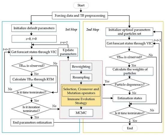
2.2.6. Data Assimilation Framework

The flowchart of the DA strategy is illustrated in Figure 1. The process of assimilation contains two stages. The long-term TB observations are used to estimate the global optimal hydrologic model parameters at the first stage, described in the blue dotted frame. In this part, the posterior distributions of the model parameters are smoothly transited from the initial sampling distribution after iteration with S steps. Then, the model parameters are updated for the next stage. Next, the aim of the second stage is the estimation of the state variables. Given VIC is the nonlinear and non-Gaussian model, the particle filter with MCMC is used to assimilate TB for SM estimation. The process of the second stage is displayed in the yellow dotted frame. Note that the two stages are evolved successively and have the same algorithm to solve the problems of particle degeneracy and impoverishment. The common processes of reweighting, resampling, and moving are illustrated in the red dotted frame. The evolution operators are based on the immune evolution strategy.

2.3. Data

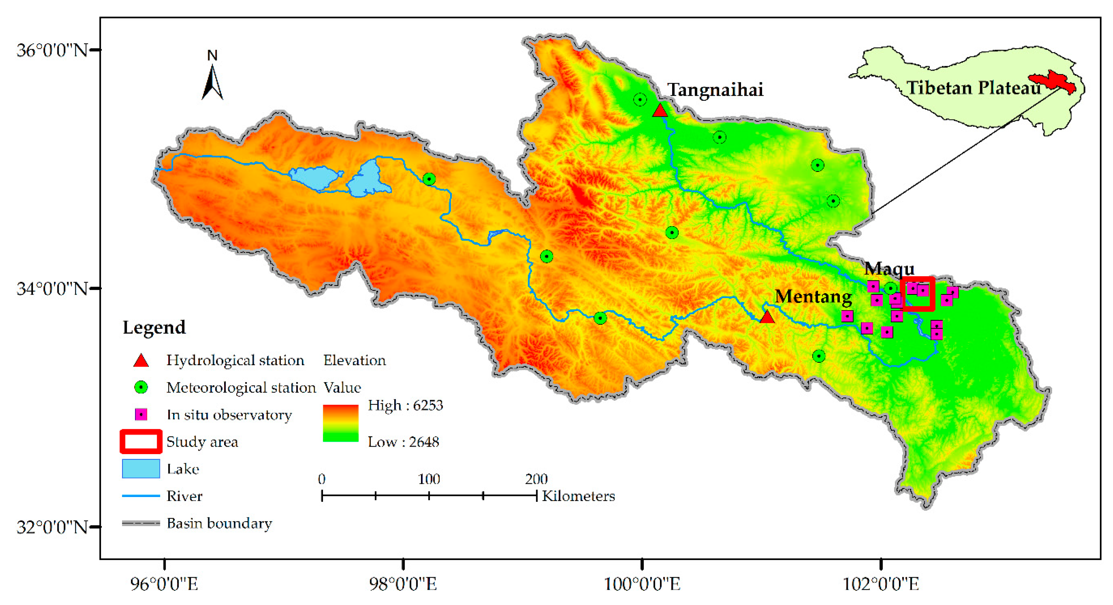
2.3.1. Study Area and In-Situ Observations

The study area is located in the Yellow River Source Region (YRSR) of China, as shown in Figure 2, which is an essential part of the National Nature Reserve of Three Rivers Source. The Yellow River originates from the eastern Tibetan Plateau, flows through the Loess Plateau, and eventually empties into the Bohai Sea [38]. It is the mother river of China and is also one of the cradles of Chinese civilization. So, understanding SM of YRSR is pivotal for water resource management, flood and irrigation management, drought warning, and even economic and policy analysis [51].
For validation purposes, in-situ observations of SM from the Maqu network are used. The Maqu observation network was established in July 2008 at the first major bend of the Yellow River (33°30′–34°15′N, 101°38′–102°45′E) for monitoring SM and soil temperature [52,53]. The network is located on the northeast edge of the Tibetan Plateau. The coverage is approximately 40   km × 80   km . For the suitable spatial area, the in-situ SM observations of this network are usually applied to validate the satellite-derived SM estimates [52,54,55]. The Maqu network covers the large valley and the hills around it. The main plant cover of the network is uniform short grassland, which is grazed by yaks and sheep. In the Maqu region, the elevation of observation stations ranges from 3200 m to 4200 m above mean sea level. Influenced by the monsoon, the region has a high and cold, moist climate, with rainy summers and dry winters. For detailed information of the Maqu network, see [52,53,54].
It is generally known that urbanization and changes in land use affect the watershed’s response to rainfall [19]. Therefore, the study area was selected far from Maqu city to satisfy the hypothesis of model parameters being invariant as much as possible. In order to enhance the simulation ability and credibility of the model, the whole region was chosen near the meteorological station to decrease the uncertainty of forcing data with similar characters. For example, land cover is grass, local topography is river valley, and soil texture is silt loam. The study area contains two in-situ observation stations named NST_06 and NST_07. The daily average soil moisture (SM) was calculated from monitoring sites as the observed SM of participating validation grid cells. Since the microwave radiation detected from space comes from the top few centimeters of the soil, in-situ measurements at depths of 5 cm and 40 cm were used to evaluate the accuracy of the surface and root zone of the SMs.

2.3.2. SMOS Brightness Temperature

SMOS is the first satellite that is specially designed for SM acquisitions by the European Space Agency (ESA). The SMOS satellite was launched on 2 November 2009. It scans the globe once every three days and crosses the equator every day at 6 a.m. and 6 p.m. local time, corresponding to ascending and descending passes, respectively. It takes advantage of fully polarized passive microwave data observed at multi-angles and retrieves SM with L-band passive microwave radiometer at a frequency of 1.4 GHz [2,56,57].
The TB datasets used for this study were the Level 1C SCLF1C TB products processing version V620. SMOS TB can be searched and downloaded at https://smos-diss.eo.esa.int/socat/SMOS_Open/. Observations are rigorously filtered for further processing, including measurements were (a) the data values must fall within the range 100–320K, (b) valid data are available for both H- and V-polarization, (c) the data are not polluted by radio frequency interference (RFI) [58]. This study specifically focused on both H- and V-polarization TBs at the nominal 42.5° incidence angle. The descending orbits of the SMOS were considered to perform the assimilation experiment over the study region during 2011 and 2012.

2.3.3. SMOS Soil Moisture Products

Satellite surface SM retrievals from SMOS were compared with the estimates by assimilation TB to further investigate the performance and behavior of the proposed methods. SMOS-IC products are developed by Institut National de la Recherche Agronomique (INRA) and Centre d’Etudes Spatiales de la BIOsphère (CESBIO) to produce the global retrievals of SM and L-vegetation optical depth (VOD). The conventional operational algorithms of SMOS level 2 and level 3 datasets are very dependent on the auxiliary files to retrieve global soil maps. Moreover, SMOS viewing geometry and the antenna pattern are accounted for in the correction. Such auxiliary files and processes increase the uncertainty of retrievals. Therefore, one of the significant targets of SMOS-IC products is to stay as independent as possible and reduce the dependence on auxiliary datasets, thus achieving more robust measurements that are less impacted by the potential uncertainties.
SMOS-IC SM products (version 105) were collected for the entire study period. The datasets are available and downloadable from https://www.catds.fr/Products/Available-products-from-CEC-SM/SMOS-IC. SM products of SMOS-IC are provided with the quality flags containing 0, 1, and 2, which stand for data OK, retrieval successful but not recommended, and missing data, respectively [59]. If SM data are strictly filtered by flag 0, the amount of data is extremely small over the YRSR. Therefore, all SMOS-IC SM datasets with quality flags 0 or 1 were used to evaluate and verify their practicality in this region.

2.3.4. Model Forcing

The version of the VIC model performed in this study was 4.2.c. In order to run the VIC model, several input datasets are required for each grid cell, such as soil information parameters, meteorological forcing files, and vegetation files. The meteorological forcing files, consisting of at least minimum and maximum temperature, wind speed, and precipitation, are obtained from the China ground climate daily dataset version 3.0. This data can be downloaded from the China Meteorological Data Service Center (http://data.cma.cn/). The vegetation information was extracted from the Maryland 1km land cover product [60]. Moreover, the soil information was extracted from the China Soil Map Based Harmonized World Soil Database (version 1.1), which is provided by the National Tibetan Plateau Data Center (http://data.tpdc.ac.cn/).

2.4. Data Assimilation Experiments

2.4.1. Experimental Design

Before the assimilation experiments started, the default parameters of the VIC model were calibrated with six years (2007–2012) of observations of streamflow data. In order to acquire the VIC model parameters of the upper Yellow River basin, streamflow simulations were performed in the whole basin at 0.25° spatial resolution, which divides the basin into 250 model grid cells. In addition, the streamflow, simulated at the basin outlet, was reprocessed with a routing model. It was a separate model using the Saint-Venant equation and employed the outputs of the VIC model grids as inputs. Then, model parameters were calibrated by iteration, optimizing model parameters and re-driving the VIC to fit simulated streamflow with observations in the same record period. The naturalized observations of streamflow were obtained from the Tangnaihai hydrologic station. The optimal parameters were considered as the default values for the model open loop (OL). Finally, the VIC model started running on 1 January 2007 to exclude the period of spin-up. Only the data starting from 31 December 2010 were used for DA experiments.
The observation error variance of SMOS is defined as 25 K2. The absolute accuracy of each station of the Maqu network is 0.02 m3m−3, following the specific calibration results [52], which can be considered as in-situ measurement error. For both steps of the assimilation experiments, the number of the particle sets was 30, and the max iteration number was 600. The other parameters of the immune evolution algorithm followed a previous study [34], including crossover and mutation probability setting values of 0.8 and 0.3, respectively.
As the first step of the assimilation strategy, the preprocessed SMOS TBs were assimilated into VIC model to estimate parameters in 2011. Then, the parameters of the VIC model were updated by estimates. The simulated SM of OL was obtained by driving the model with the updated parameters in 2012. In addition, the available SMOS TBs were assimilated into the VIC with the same estimated parameters to estimate the SM in the same period. The different simulated SMs are analyzed and discussed with the model OL and in-situ measurements in the following section.

2.4.2. Evaluation Metrics

In this paper, three deterministic metrics were selected to evaluate the performance of the assimilation experiments, including the root mean square error (RMSE), the mean bias error (MBE) and the correlation coefficient (R):
R M S E = 1 n t = 1 n ( S M e s t t S M o b s t ) 2 ,
M B E = 1 n t = 1 n ( S M e s t t S M o b s t ) ,
R = t = 1 n ( S M e s t t S M e s t ¯ ) ( S M o b s t S M o b s ¯ ) t = 1 n ( S M e s t t S M e s t ¯ ) 2 t = 1 n ( S M o b s t S M o b s ¯ ) 2 ,
where n is the step number; S M e s t t and S M o b s t represent estimated SM and in-situ observations of SM at step t, respectively. S M e s t ¯ and S M o b s ¯ denote corresponding mean values.

3. Results

3.1. Evaluation of Parameters Estimation

The model parameters estimation was performed for the VIC simulation with the full energy balance and frozen soils mode. According to the suggestion that the optimization time window of one year for model calibration is reasonably rational for the Maqu region [17] and the assumption that model parameters are time-invariant in the short term, the preprocessed TBs were assimilated into the VIC model from March to September in 2011, including soil freezing/thawing and unfrozen periods (from May to September). The experiment of the first strategy for parameters estimation independently ran 30 times, which provided stable estimates of the parameters. The average values were considered as optimal values. The initial parameters values for the model simulation were assumed with a uniform prior distribution of their corresponding range values.
One of the experiments was selected to analyze the processes of parameters estimation. The particles tracking paths of the model parameters are illustrated in Figure 3 to help understand the convergence status of the immune evolution strategy. It is not difficult to see that in the initial stages, the magenta particles randomly distributed in the whole parameter space. The transitions of the sampling seemed to be efficient at exploring the solution space. With increasing iterations, all particles tended towards convergence with a limiting distribution that seemed relatively tight. Except for parameters of B and d3, the other estimates were close to the default parameter values, represented by the red circle at the right y-axis. This is perhaps to be expected, as the likelihood function of two estimation methods is calculated based on the different observations with TB or streamflow. The difference of optimal model parameters influences the SM simulation.
As presented in Figure 4, the time series of surface SM simulated with optimal and default parameters were compared with the in-situ observations from 2011 (calibration period) to those of 2012 (validation period), which was used to evaluate the parameters estimated by assimilation SMOS TB. The daily precipitation data are displayed by stem plots in the simulation period. Overall, SMs simulated by the two parameters sets were very similar. They were able to reflect the changing trend of the topsoil SM in an unfrozen period. Note that the gap between the simulated SM and the observations was remarkable during the period of soil thawing. In addition, it can be clearly seen that strong consistency exists between the simulation and the precipitation. Although all simulation SMs are lower than in-situ observations, the SM simulated with optimal parameters was closer than that using the default values. This indicates that assimilating SMOS TB is indeed helpful for hydrologic parameter estimation. Among the parameters, B was the most sensitive parameter, and the second was the thickness of the second soil layer d2. This is because those two parameters can directly impact on the soil water storage capacity, which influences the runoff route [39]. Thus, the value of B is the major cause impacting the surface SM. More detailed information based on the deterministic metrics will be discussed in the next section.

3.2. Evaluation of Soil Moisture Estimation

In the second strategy, SMOS TB data were assimilated into the VIC model with the optimal parameters estimated in the first step. The assimilation time window was chosen to be from March to September in 2012. Although the available TB data in soil thawing period was very restricted, the experiment tried to obtain the surface SM and assess the performance of assimilation TB.
Figure 5 presents the comparison of daily SMs including in-situ observations, the open loop with estimated parameters (OL_opt), open loop with default parameters (OL_def), and the simulations by the assimilation SMOS TB with estimated parameters (DA_opt). During the simulation period, the simulated SM was clearly underestimated, both in the open loop and assimilation TB. The reason for the underestimation results at the grid cell may be explained by not only the scale transformation of the representativeness from a 0.25 degree grid to a region observation, but also intrinsic limitations of the input variables. The underestimation is a common deficiency by hydrologic models in this region [17], especially in soil thawing/freezing periods. The magenta line seems to change more rapidly in the beginning of the assimilation period. This is possibly because the processes of soil thawing/freezing alternate dramatically, and the model of soil dielectric is no longer suitable in the frozen condition.
Table 2 summarizes the performance of OL_opt, OL_def, and DA_opt in the unfrozen period and the entire simulation period, respectively. According to the deterministic measures, OL_opt (RMSE = 0.077 m3m−3, MBE = 0.074 m3m−3) and DA_opt (RMSE = 0.088 m3m−3, MBE = 0.073 m3m−3) show higher accuracy than OL_def (RMSE = 0.108 m3m−3, MBE = 0.105 m3m−3) at a grid scale in the unfrozen period. The same result was also found in the entire simulation period. It indicates that assimilation of SMOS TB into the VIC with an immune evolution strategy can improve the performance of SM estimates. Considering frozen soil both in OL_opt and DA_opt, DA_opt (RMSE = 0.087 m3m−3, MBE = 0.059 m3m−3, R = 0.808) obtains the best performance in the entire simulation period. This explains the need to divide the assimilation experiment into two steps in the DA scheme. Assimilation TB for model parameters ensured the rationality and usability of the model as a whole in the study region. Then, assimilation with the available TB for the model state variables estimation with updated parameters improved the estimation accuracy at a daily timestep.
Figure 6 shows Taylor diagrams for the in-situ validation of OL_opt (A), OL_def (B), and DA_opt (C). Taylor diagrams reveal a very similar standard deviation or correlation coefficient of OL_opt and OL_def, no matter which period is analyzed. However, the standard deviation of DA_opt changes from close to OL_opt and OL_def to smaller than them, and R increases to above 0.8 over the whole year. This indicates that DA_opt improved the performance of the SM simulation except for during the unfrozen period. These findings correspond well to Figure 5.

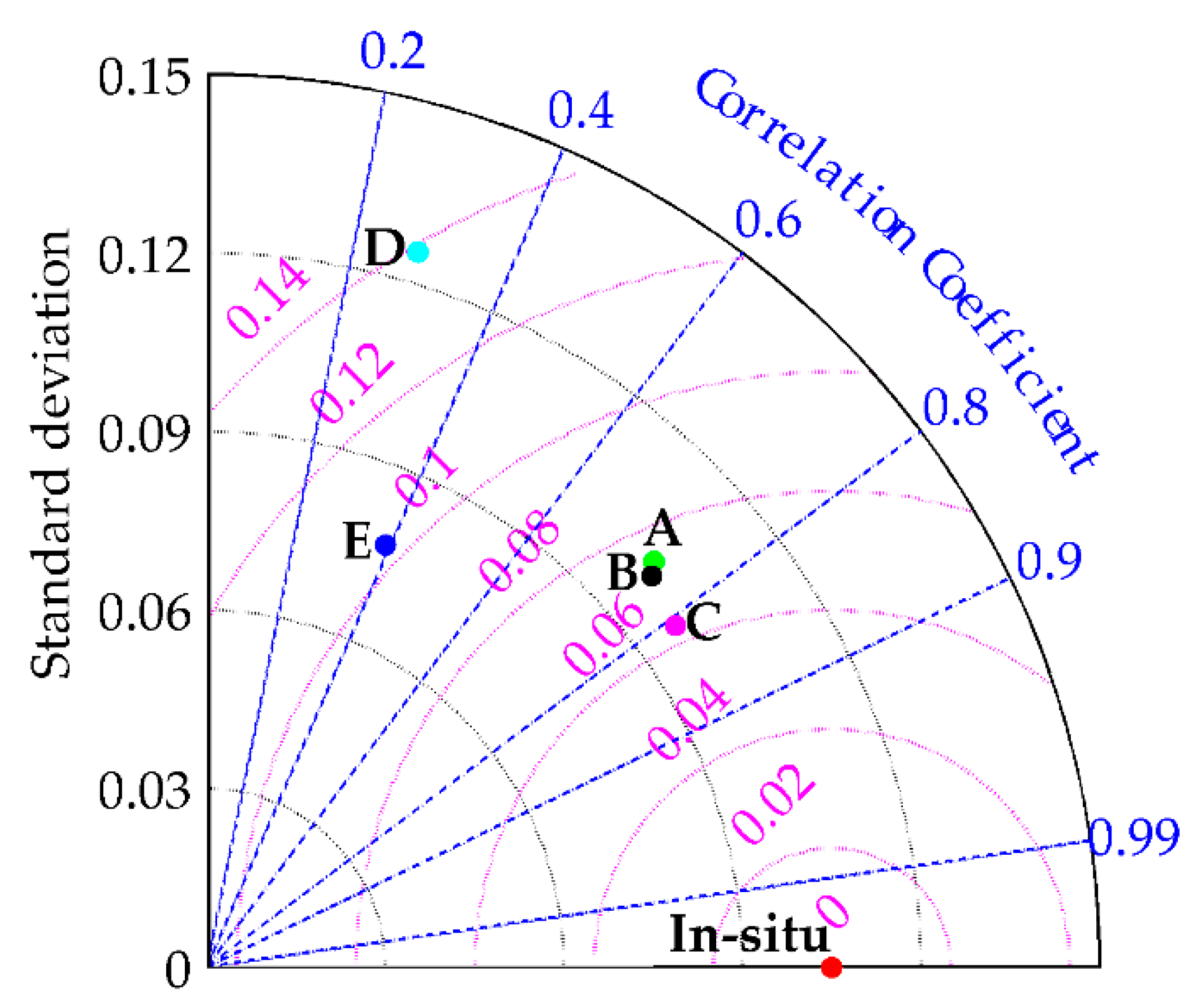
3.3. Comparison with Other Soil Moisture Estimations

The estimation results of the assimilation were compared with SMOS-IC products to further evaluate the effectiveness of the DA scheme based on the immune evolutionary strategy in 2012. Since TB can only reflect the radiative characteristics of the topsoil, the simulated SM data of top layer and SMOS-IC were compared with in-situ measurements. It should be noted that the available SMOS-IC products in the study area were very restricted; therefore, all SMOS-IC data in the whole period of 2012 are illustrated for comparison. Ascending and descending products of SMOS-IC were separately compared with observations. Figure 7 presents the scatter plots of SMOS retrievals and assimilation results. Overall, the performance of DA_opt and OL_opt was better than SMOS-IC products. Furthermore, compared with the descending products, the ascending products had four records reaching up to about 0.6 m3m−3. The unreliable estimated SM may originate from SMOS observations contaminated by RFI.
Figure 8 displays the statistics of the comparison of the estimated SMs and SMOS-IC products. Both SMOS-IC_ASC (D) and SMOS-IC_DES (E) had larger standard deviation and lower correlation coefficients than the model estimation. This larger standard deviation indicates that their variability was greater than that of the in-situ measurements. The same conclusion was also found by some other studies [55,61]. The correlation coefficients of the model simulated data sets were larger than 0.74, which implies a good ability of capturing the dynamic change of SM observations. The root mean square error difference (RMSD) of DA_opt was close to 0.06 m3m−3, which implies that there was not a significant bias in DA_opt. The results suggest that the estimated SM by assimilation was better than SMOS-IC in this region.

3.4. Comparison with Root Zone SM Estimates

To investigate the effect of assimilation TB on estimation of the SM of the root zone, the in-situ observation at a depth of 40cm was chosen as the calibration data set from May to September. Figure 9 illustrates the comparison of simulated SM time series with and without assimilation TB. Generally, the fluctuation of root zone SM is more gentler than that of the surface SM shown in Figure 5. Clearly, all SM sets can reflect two massive precipitation events in July, with the total amount of precipitation being larger than 30mm per day. This indicates that the precipitation was the most sensitive forcing data for SM in both the surface and root zone of the soil. Moreover, the red and magenta lines show more variation to the precipitation. This means that both observation and DA_opt can capture more precipitation events.
Table 3 shows the performance of root zone SM sets. In terms of R value, DA_opt (R=0.755) shows the best performance. This finding is the same as the plot in Figure 9. However, both RMSE and MBE of DA_opt are the largest. In terms of the observation data, DA_opt slightly overestimates root zone SM, which is the opposite trend to the surface SM. This overestimation phenomenon may be explained by the compensating underestimation phenomenon at the surface soil to keep water balance in the VIC model. It depends on the water transfer mechanism and the model parameters of VIC. Nonetheless, the RMSE value of DA_opt (RMSE = 0.029 m3m−3) falls within the time domain reflectometry (TDR) local measurement probe errors. According to R and RMSE values, the root zone SM time series also achieved satisfying results by assimilation of the microwave observations at the surface soil layer.

4. Discussion

In general, the surface SM profiles simulated with estimated and default parameters showed similar trends compared with in-situ measurements. The significant difference between the simulated SM and the observations could not be eliminated during the soil thawing period with assimilation TB or streamflow. One possible reason is that the optimal parameters for the entire year are not suitable for the freezing/thawing period. The hypothesis that the model parameters are time-invariant might not be justified when the soil status changes. This means that the static parameters have their own time attribute. Yang et al. conducted the optimization of static model parameters using AMSR-E TB data only for the unfrozen period on the Tibetan Plateau [17]. In fact, the hydrology of YRSR in the real world is very complex, the hydrological model cannot simulate it sufficiently, especially with regard to soil freezing and thawing processes.
In this study, the DA strategy had two stages, which were performed in a successive and unidirectional manner. As shown in Table 2, RMSE of OL_opt increased from 0.077 to 0.102 m3m−3 in different statistic periods, transiting from unfrozen to the entire simulation period. RMSE of DA_opt decreased from 0.088 to 0.087 m3m−3 and changed little. Although the available TB data are limited, assimilation TB observation can improve SM estimation in the thawing period. However, both RMSE and R of OL_opt performed better than DA_opt in the unfrozen period. The second step may increase or decrease RMSE in unfrozen and frozen periods. The new SM dataset blending OL_opt in the entire simulation period and DA_opt in the freezing/thawing period was a viable option for practice application. It also reflects the effectiveness of the two-stage DA strategy from a sideways perspective. Specifically, Table 3 reveals the opposite changing trend of RMSE and R in the unfrozen period, which is different from Table 2. RMSE decreased from 0.108 to 0.077 m3m−3 for surface SM, and increased from 0.021 to 0.029 m3m−3 for root zone SM. The amount of change slightly increased for the root zone. It is not difficult to see that assimilation for surface SM has a smaller impact on RMSE than on the root zone. This may also be explained by the estimates of model parameters that can meet the local measurement accuracy. Moreover, the temporal correlation between DA results and in-situ measurements increased to 0.755 for root zone SM (+0.040), which means estimates can respond better to changes of root zone SM, as shown in Figure 9.
Obviously, both ascending and descending SMOS-IC products significantly underestimated SM and had inferior accuracy in the study region, which was also found by some other studies [55,62]. This bias is generally negative as satellite data usually fails across extremely dry or extremely humid conditions. Moreover, the uncertainties of SMOS-IC products mainly derive from the observation error and the inversion algorithms, which may not be very effective in this region. The main factors, including the physical temperatures of soil and vegetation, vegetation optical parameters, albedo parameters, soil permittivity, and surface roughness, influence the performances of the satellite SM products [59]. As mentioned in Section 2.1.2, the important parameter τ that combines roughness and vegetation is canceled by formulas (6) and (7), which may decrease the uncertainties during estimating SM.
It should be noted that only two SM ground observation stations were selected to evaluate the effectiveness of the DA framework based on immune evolutionary strategy, which has some limitations. All the observational data are near Maqu city, which is mostly flat and lacks representativeness of upland areas. In the soil thawing/freezing period, the runoff generated from snowy mountains has significant influence on SM of upland areas on the Tibetan Plateau. More and different geography conditions need to be considered for evaluation in the future.

5. Conclusions

This paper investigated the effectiveness of directly assimilating SMOS TB into a distributed hydrological model for the estimation of time-invariant model parameters and dynamic SM with an immune evolutionary strategy. The assimilation experiments were implemented through two-step processes at a grid scale. Estimation of parameters was conducted for one year, and estimation of SM was carried out over the next year. The results of assimilation experiments were evaluated by in-situ observation of the Maqu network, located on the northeast edge of the Tibetan Plateau. Specifically, surface SM time series (RMSE = 0.102 m3m−3, R = 0.741) simulated with optimal parameters performed better than SMs (RMSE = 0.126 m3m−3, R = 0.751) simulated with default parameters. Then, assimilation TB for model state estimation with updated parameters improved the performance of the SM set (RMSE = 0.087 m3m−3, R = 0.808) in the whole simulation period. Assimilation TB also had a smaller positive impact on the root zone layer. These results are quite encouraging in joint estimation of parameters and state variables based on assimilation microwave observations instead of streamflow or in-situ measurement at a grid scale.
Although the VIC model operates with a frozen soils mode, underestimation of the surface SM profile simulated with or without updated parameters was a common phenomenon in this area, especially in the freezing/thawing period from March to April. The complexity of the freezing/thawing processes in the real world and the limitations in model structure means the VIC model is unable to simulate SM sufficiently. Assimilation of microwave observations into the model only reduced the bias to the measurement, but cannot fundamentally solve the problems. The estimated parameters using TB observations were optimal for the entire year, but not suitable for the freezing/thawing period. This also explains the necessity of designing two strategies for estimating model parameters and state variables in this study. An excellent model parameter optimal scheme with time-variant model parameters for different frozen and unfrozen periods is expected in further research. However, the assimilation strategy based on an immune evolutionary strategy is still appropriate.
Moreover, SMOS-IC products were compared with assimilation results. Both ascending and descending SMOS-IC products also significantly underestimated values and had lower accuracy than the assimilation results. The use of SMOS-IC products must be done carefully in this region in further studies.
In summary, this paper presents the high potential to estimate model parameters and state variables through microwave TB observations assimilation based on the immune evolutionary strategy at a grid scale. Future work on assimilation remote sensing data are recommended in two aspects. First, multiple passive microwave remote sensing data, such as surface temperature products, should be assimilated and multi-objective optimal techniques should be applied in the assimilation scheme. In addition, the immune evolutionary strategy should be verified in different climate and environmental conditions.

Author Contributions

Conceptualization, F.J. and R.A.; Formal analysis, Z.Y.; Funding acquisition, R.A.; Investigation, F.J.; Methodology, F.J. and R.A.; Resources, Z.Y.; Software, F.J. and L.H.; Validation, L.H. and Y.S.; Writing—original draft, F.J.; Writing—review and editing, R.A. and Z.Y. All authors have read and agreed to the published version of the manuscript.

Funding

This research was partially funded by the National Natural Science Foundation of China, grant numbers 41871326, 41271361, and 61903139.

Acknowledgments

The authors are grateful to the ESA and CESBIO for making SMOS TB and SMOS-IC products available, and thankful to the China Meteorological Data Service Center and National Tibetan Plateau Data Center for providing meteorological data and soil data, and also grateful to Su and Zeng for kindly providing the in-situ measurements. The authors also thank three anonymous reviews for their critical comments and constructive suggestions.

Conflicts of Interest

The authors declare no conflict of interest.

References

  1. Rains, D.; De Lannoy, G.J.M.; Lievens, H.; Walker, J.P.; Verhoest, N.E.C. SMOS and SMAP Brightness Temperature Assimilation Over the Murrumbidgee Basin. IEEE Geosci. Remote Sens. Lett. 2018, 15, 1652–1656. [Google Scholar] [CrossRef]
  2. Parrens, M.; Wigneron, J.-P.; Richaume, P.; Mialon, A.; Al Bitar, A.; Fernandez-Moran, R.; Al-Yaari, A.; Kerr, Y.H. Global-scale surface roughness effects at L-band as estimated from SMOS observations. Remote Sens. Environ. 2016, 181, 122–136. [Google Scholar] [CrossRef]
  3. Brocca, L.; Ciabatta, L.; Massari, C.; Camici, S.; Tarpanelli, A. Soil Moisture for Hydrological Applications: Open Questions and New Opportunities. Water 2017, 9, 140. [Google Scholar] [CrossRef]
  4. Kirby, J.M.; Mainuddin, M.; Ahmad, M.D.; Gao, L. Simplified Monthly Hydrology and Irrigation Water Use Model to Explore Sustainable Water Management Options in the Murray-Darling Basin. Water Resour. Manag. 2013, 27, 4083–4097. [Google Scholar] [CrossRef]
  5. Moradkhani, H. Hydrologic remote sensing and land surface data assimilation. Sensors 2008, 8, 2986–3004. [Google Scholar] [CrossRef] [PubMed]
  6. Huang, C.; Xin, L.; Ling, L. Retrieving soil temperature profile by assimilating MODIS LST products with ensemble Kalman filter. Remote Sens. Environ. 2008, 112, 1320–1336. [Google Scholar] [CrossRef]
  7. Dumedah, G.; Coulibaly, P. Evolutionary assimilation of streamflow in distributed hydrologic modeling using in-situ soil moisture data. Adv. Water Resour. 2013, 53, 231–241. [Google Scholar] [CrossRef]
  8. Kolassa, J.; Reichle, R.H.; Draper, C.S. Merging active and passive microwave observations in soil moisture data assimilation. Remote Sens. Environ. 2017, 191, 117–130. [Google Scholar] [CrossRef]
  9. Rains, D.; Han, X.J.; Lievens, H.; Montzka, C.; Verhoest, N.E.C. SMOS brightness temperature assimilation into the Community Land Model. Hydrol. Earth Syst. Sci. 2017, 21, 5929–5951. [Google Scholar] [CrossRef] [Green Version]
  10. Gruber, A.; Lannoy, G.D.; Crow, W. A Monte Carlo based adaptive Kalman filtering framework for soil moisture data assimilation. Remote Sens. Environ. 2019, 228, 105–114. [Google Scholar] [CrossRef]
  11. Nair, A.S.; Indu, J. Improvement of land surface model simulations over India via data assimilation of satellite-based soil moisture products. J. Hydrol. 2019, 573, 406–421. [Google Scholar] [CrossRef]
  12. Bi, H.; Ma, J.; Wang, F. An Improved Particle Filter Algorithm Based on Ensemble Kalman Filter and Markov Chain Monte Carlo Method. IEEE Trans. Geosci. Remote Sens. 2015, 53, 6134–6147. [Google Scholar] [CrossRef]
  13. Blankenship, C.B.; Case, J.L.; Zavodsky, B.T.; Crosson, W.L. Assimilation of SMOS Retrievals in the Land Information System. IEEE Trans. Geosci. Remote Sens. 2016, 54, 6320–6332. [Google Scholar] [CrossRef] [Green Version]
  14. Yan, H.; Moradkhani, H. Combined assimilation of streamflow and satellite soil moisture with the particle filter and geostatistical modeling. Adv. Water Resour. 2016, 94, 364–378. [Google Scholar] [CrossRef] [Green Version]
  15. De Lannoy, G.J.M.; Reichle, R.H. Global Assimilation of Multiangle and Multipolarization SMOS Brightness Temperature Observations into the GEOS-5 Catchment Land Surface Model for Soil Moisture Estimation. J. Hydrometeorol. 2016, 17, 669–691. [Google Scholar] [CrossRef] [Green Version]
  16. Kan, G.Y.; He, X.Y.; Li, J.R.; Ding, L.Q.; Hong, Y.; Zhang, H.B.; Liang, K.; Zhang, M.J. Computer Aided Numerical Methods for Hydrological Model Calibration: An Overview and Recent Development. Arch. Comput. Method Eng. 2019, 26, 35–59. [Google Scholar] [CrossRef]
  17. Yang, K.; Zhu, L.; Chen, Y.Y.; Zhao, L.; Qin, J.; Lu, H.; Tang, W.J.; Han, M.L.; Ding, B.H.; Fang, N. Land surface model calibration through microwave data assimilation for improving soil moisture simulations. J. Hydrol. 2016, 533, 266–276. [Google Scholar] [CrossRef]
  18. Chen, W.J.; Shen, H.F.; Huang, C.L.; Li, X. Improving Soil Moisture Estimation with a Dual Ensemble Kalman Smoother by Jointly Assimilating AMSR-E Brightness Temperature and MODIS LST. Remote Sens. 2017, 9, 273. [Google Scholar] [CrossRef] [Green Version]
  19. Vrugt, J.A.; ter Braak, C.J.F.; Diks, C.G.H.; Schoups, G. Hydrologic data assimilation using particle Markov chain Monte Carlo simulation: Theory, concepts and applications. Adv. Water Resour. 2013, 51, 457–478. [Google Scholar] [CrossRef]
  20. Zhu, G.F.; Li, X.; Ma, J.Z.; Wang, Y.Q.; Liu, S.M.; Huang, C.L.; Zhang, K.; Hu, X.L. A new moving strategy for the sequential Monte Carlo approach in optimizing the hydrological model parameters. Adv. Water Resour. 2018, 114, 164–179. [Google Scholar] [CrossRef]
  21. Moradkhani, H.; Dechant, C.M.; Sorooshian, S. Evolution of ensemble data assimilation for uncertainty quantification using the particle filter-Markov chain Monte Carlo method. Water Resour. Res. 2012, 48, 120. [Google Scholar] [CrossRef]
  22. Moradkhani, H.; Hsu, K.L.; Gupta, H.; Sorooshian, S. Uncertainty assessment of hydrologic model states and parameters: Sequential data assimilation using the particle filter. Water Resour. Res. 2005, 41, 388. [Google Scholar] [CrossRef] [Green Version]
  23. Abbaszadeh, P.; Moradkhani, H.; Yan, H.X. Enhancing hydrologic data assimilation by evolutionary Particle Filter and Markov Chain Monte Carlo. Adv. Water Resour. 2018, 111, 192–204. [Google Scholar] [CrossRef]
  24. Fan, Y.; Leslie, D.S.; Wand, M.P. Generalised linear mixed model analysis via sequential Monte Carlo sampling. Electron. J. Stat. 2008, 2, 916–938. [Google Scholar] [CrossRef]
  25. Jeremiah, E.; Sisson, S.; Marshall, L.; Mehrotra, R.; Sharma, A. Bayesian calibration and uncertainty analysis of hydrological models: A comparison of adaptive Metropolis and sequential Monte Carlo samplers. Water Resour. Res. 2011, 47, 33. [Google Scholar] [CrossRef]
  26. Jeremiah, E.; Sisson, S.A.; Sharma, A.; Marshall, L. Efficient hydrological model parameter optimization with Sequential Monte Carlo sampling. Environ. Model. Softw. 2012, 38, 283–295. [Google Scholar] [CrossRef]
  27. Brocca, L.; Moramarco, T.; Melone, F.; Wagner, W.; Hasenauer, S.; Hahn, S. Assimilation of Surface- and Root-Zone ASCAT Soil Moisture Products into Rainfall-Runoff Modeling. IEEE Trans. Geosci. Remote Sens. 2012, 50, 2542–2555. [Google Scholar] [CrossRef]
  28. Samuel, J.; Coulibaly, P.; Dumedah, G.; Moradkhani, H. Assessing model state and forecasts variation in hydrologic data assimilation. J. Hydrol. 2014, 513, 127–141. [Google Scholar] [CrossRef]
  29. DeChant, C.M.; Moradkhani, H. Examining the effectiveness and robustness of sequential data assimilation methods for quantification of uncertainty in hydrologic forecasting. Water Resour. Res. 2012, 48, 106. [Google Scholar] [CrossRef] [Green Version]
  30. Hartanto, I.M.; van der Kwast, J.; Alexandridis, T.K.; Almeida, W.; Song, Y.; van Andel, S.J.; Solomatine, D.P. Data assimilation of satellite-based actual evapotranspiration in a distributed hydrological model of a controlled water system. Int. J. Appl. Earth Obs. Geoinf. 2017, 57, 123–135. [Google Scholar] [CrossRef]
  31. Zhang, H.J.; Franssen, H.J.H.; Han, X.J.; Vrugt, J.A.; Vereecken, H. State and parameter estimation of two land surface models using the ensemble Kalman filter and the particle filter. Hydrol. Earth Syst. Sci. 2017, 21, 4927–4958. [Google Scholar] [CrossRef] [Green Version]
  32. Vrugt, J.A. Markov chain Monte Carlo simulation using the DREAM software package: Theory, concepts, and MATLAB implementation. Environ. Model. Softw. 2016, 75, 273–316. [Google Scholar] [CrossRef] [Green Version]
  33. Andrieu, C.; Doucet, A.; Holenstein, R. Particle Markov chain Monte Carlo methods. J. R. Stat. Soc. 2010, 72, 269–342. [Google Scholar] [CrossRef] [Green Version]
  34. Ju, F.; An, R.; Sun, Y.X. Immune Evolution Particle Filter for Soil Moisture Data Assimilation. Water 2019, 11, 211. [Google Scholar] [CrossRef] [Green Version]
  35. Penny, S.G.; Miyoshi, T. A local particle filter for high-dimensional geophysical systems. Nonlinear Process. Geophys. 2016, 23, 391–405. [Google Scholar] [CrossRef] [Green Version]
  36. Zhu, M.B.; van Leeuwen, P.J.; Amezcua, J. Implicit equal-weights particle filter. Q. J. R. Meteorol. Soc. 2016, 142, 1904–1919. [Google Scholar] [CrossRef] [Green Version]
  37. Liang, X.; Lettenmaier, D.P.; Wood, E.F.; Burges, S.J. A simple hydrologically based model of land surface water and energy fluxes for general circulation models. J. Geophys. Res. Atmos. 1994, 99, 14415–14428. [Google Scholar] [CrossRef]
  38. Su, J.B.; Lu, H.S.; Wang, J.Q.; Sadeghi, A.M.; Zhu, Y.H. Evaluating the Applicability of Four Latest Satellite-Gauge Combined Precipitation Estimates for Extreme Precipitation and Streamflow Predictions over the Upper Yellow River Basins in China. Remote Sens. 2017, 9, 1176. [Google Scholar] [CrossRef] [Green Version]
  39. Chen, Y.Y.; Niu, J.; Kang, S.Z.; Zhang, X.T. Effects of irrigation on water and energy balances in the Heihe River basin using VIC model under different irrigation scenarios. Sci. Total Environ. 2018, 645, 1183–1193. [Google Scholar] [CrossRef]
  40. Park, D.; Markus, M. Analysis of a changing hydrologic flood regime using the Variable Infiltration Capacity model. J. Hydrol. 2014, 515, 267–280. [Google Scholar] [CrossRef]
  41. Troy, T.J.; Wood, E.F.; Sheffield, J. An efficient calibration method for continental-scale land surface modeling. Water Resour. Res. 2008, 44, 93. [Google Scholar] [CrossRef]
  42. Tesemma, Z.K.; Wei, Y.; Peel, M.C.; Western, A.W. The effect of year-to-year variability of leaf area index on Variable Infiltration Capacity model performance and simulation of runoff. Adv. Water Resour. 2015, 83, 310–322. [Google Scholar] [CrossRef] [Green Version]
  43. Lievens, H.; Al Bitar, A.; Verhoest, N.E.C.; Cabot, F.; De Lannoy, G.J.M.; Drusch, M.; Dumedah, G.; Franssen, H.J.H.; Kerr, Y.; Tomer, S.K.; et al. Optimization of a Radiative Transfer Forward Operator for Simulating SMOS Brightness Temperatures over the Upper Mississippi Basin. J. Hydrometeorol. 2015, 16, 1109–1134. [Google Scholar] [CrossRef] [Green Version]
  44. Parrens, M.; Wigneron, J.P.; Richaume, P.; Al Bitar, A.; Mialon, A.; Fernandez-Moran, R.; Al-Yaari, A.; O’Neill, P.; Kerr, Y. Considering combined or separated roughness and vegetation effects in soil moisture retrievals. Int. J. Appl. Earth Obs. Geoinf. 2017, 55, 73–86. [Google Scholar] [CrossRef]
  45. Mironov, V.; Kerr, Y.; Wigneron, J.P.; Kosolapova, L.; Demontoux, F. Temperature- and Texture-Dependent Dielectric Model for Moist Soils at 1.4 GHz. IEEE Geosci. Remote Sens. Lett. 2013, 10, 419–423. [Google Scholar] [CrossRef] [Green Version]
  46. Arulampalam, M.S.; Maskell, S.; Gordon, N.; Clapp, T. A tutorial on particle filters for online nonlinear/non-Gaussian Bayesian tracking. IEEE Trans. Signal Process. 2002, 50, 174–188. [Google Scholar] [CrossRef] [Green Version]
  47. Owen, A.B.; Tribble, S.D. A quasi-Monte Carlo Metropolis algorithm. Proc. Natl. Acad. Sci. USA 2005, 102, 8844–8849. [Google Scholar] [CrossRef] [Green Version]
  48. Yang, Z.; Ding, Y.S.; Hao, K.R.; Cai, X. An adaptive immune algorithm for service-oriented agricultural Internet of Things. Neurocomputing 2019, 344, 3–12. [Google Scholar] [CrossRef]
  49. Yang, Z.; Ding, Y.S.; Jin, Y.C.; Hao, K.R. Immune-Endocrine System Inspired Hierarchical Coevolutionary Multiobjective Optimization Algorithm for IoT Service. IEEE Trans. Cybern. 2020, 50, 164–177. [Google Scholar] [CrossRef]
  50. Han, H.; Ding, Y.S.; Hao, K.R.; Liang, X. An evolutionary particle filter with the immune genetic algorithm for intelligent video target tracking. Comput. Math. Appl. 2011, 62, 2685–2695. [Google Scholar] [CrossRef] [Green Version]
  51. Bryan, B.A.; Gao, L.; Ye, Y.Q.; Sun, X.F.; Connor, J.D.; Crossman, N.D.; Stafford-Smith, M.; Wu, J.G.; He, C.Y.; Yu, D.Y.; et al. China’s response to a national land-system sustainability emergency. Nature 2018, 559, 193–204. [Google Scholar] [CrossRef]
  52. Su, Z.; Wen, J.; Dente, L.; van der Velde, R.; Wang, L.; Ma, Y.; Yang, K.; Hu, Z. The Tibetan Plateau observatory of plateau scale soil moisture and soil temperature (Tibet-Obs) for quantifying uncertainties in coarse resolution satellite and model products. Hydrol. Earth Syst. Sci. 2011, 15, 2303–2316. [Google Scholar] [CrossRef] [Green Version]
  53. Dente, L.; Vekerdy, Z.; Wen, J.; Su, Z. Maqu network for validation of satellite-derived soil moisture products. Int. J. Appl. Earth Obs. Geoinf. 2012, 17, 55–65. [Google Scholar] [CrossRef]
  54. Laura, D.; Zhongbo, S.; Jun, W. Validation of SMOS soil moisture products over the Maqu and Twente regions. Sensors 2012, 12, 9965–9986. [Google Scholar]
  55. Zeng, J.Y.; Li, Z.; Chen, Q.; Bi, H.Y.; Qiu, J.X.; Zou, P.F. Evaluation of remotely sensed and reanalysis soil moisture products over the Tibetan Plateau using in-situ observations. Remote Sens. Environ. 2015, 163, 91–110. [Google Scholar] [CrossRef]
  56. Kerr, Y.H.; Waldteufel, P.; Richaume, P.; Wigneron, J.P.; Ferrazzoli, P.; Mahmoodi, A.; Al Bitar, A.; Cabot, F.; Gruhier, C.; Juglea, S.E.; et al. The SMOS Soil Moisture Retrieval Algorithm. IEEE Trans. Geosci. Remote Sens. 2012, 50, 1384–1403. [Google Scholar] [CrossRef]
  57. Fernandez-Moran, R.; Wigneron, J.P.; De Lannoy, G.; Lopez-Baeza, E.; Parrens, M.; Mialon, A.; Mahmoodi, A.; Al-Yaari, A.; Bircher, S.; Al Bitar, A.; et al. A new calibration of the effective scattering albedo and soil roughness parameters in the SMOS SM retrieval algorithm. Int. J. Appl. Earth Obs. Geoinf. 2017, 62, 27–38. [Google Scholar] [CrossRef]
  58. De Lannoy, G.J.M.; Reichle, R.H. Assimilation of SMOS brightness temperatures or soil moisture retrievals into a land surface model. Hydrol. Earth Syst. Sci. 2016, 20, 4895–4911. [Google Scholar] [CrossRef] [Green Version]
  59. Liu, J.; Chai, L.N.; Lu, Z.; Liu, S.M.; Qu, Y.Q.; Geng, D.Y.; Song, Y.Z.; Guan, Y.B.; Guo, Z.X.; Wang, J.; et al. Evaluation of SMAP, SMOS-IC, FY3B, JAXA, and LPRM Soil Moisture Products over the Qinghai-Tibet Plateau and Its Surrounding Areas. Remote Sens. 2019, 11, 792. [Google Scholar] [CrossRef] [Green Version]
  60. Hansen, M.C.; Defries, R.S.; Townshend, J.R.G.; Sohlberg, R. Global land cover classification at 1km spatial resolution using a classification tree approach. Int. J. Remote Sens. 2000, 21, 1331–1364. [Google Scholar] [CrossRef]
  61. Zeng, Y.J.; Su, Z.B.; van der Velde, R.; Wang, L.C.; Xu, K.; Wang, X.; Wen, J. Blending Satellite Observed, Model Simulated, and in Situ Measured Soil Moisture over Tibetan Plateau. Remote Sens. 2016, 8, 268. [Google Scholar] [CrossRef] [Green Version]
  62. Chen, Y.Y.; Yang, K.; Qin, J.; Cui, Q.; Lu, H.; La, Z.; Han, M.L.; Tang, W.J. Evaluation of SMAP, SMOS, and AMSR2 soil moisture retrievals against observations from two networks on the Tibetan Plateau. J. Geophys. Res. Atmos. 2017, 122, 5780–5792. [Google Scholar] [CrossRef]
Figure 1. The flowchart of the data assimilation strategy.
Remotesensing 12 01556 g001
Figure 2. The location of the Yellow River Source Region and study area (red rectangle).
Remotesensing 12 01556 g002
Figure 3. Trace of the model parameters. The magenta points represent the sampling particles of the parameters. The blue line is the mean value of particles. The red circle at the right y-axis is the default parameter value.
Remotesensing 12 01556 g003
Figure 4. Comparison of surface SMs between the observations and the simulations with different model parameters.
Remotesensing 12 01556 g004
Figure 5. The comparison of surface SM time series for in-situ observations, the open loop with estimated parameters (OL_opt), open loop with default parameters (OL_def), and the simulations by the assimilation SMOS TB with estimated parameters (DA_opt).
Remotesensing 12 01556 g005
Figure 6. Taylor diagram illustrating the statistics of the comparison between the observed measurement and simulation in terms of correlation coefficient R and standard deviation. Results show the (a) unfrozen period and (b) entire simulation period. The in-situ data are displayed by red markers; OL_def and OL_opt are represented by black and green markers, respectively; DA_opt is denoted by magenta markers.
Remotesensing 12 01556 g006
Figure 7. Scatter plots of the simulation SM sets and SMOS-IC products.
Remotesensing 12 01556 g007
Figure 8. Taylor diagram illustrating the statistics of the comparison, including the in-situ measurement, the simulation SM sets, and SMOS-IC products in terms of correlation coefficient R, standard deviation, and root mean square error difference. SMOS-IC_ASC and SMOS-IC_DES are represented by cyan and blue markers, respectively.
Remotesensing 12 01556 g008
Figure 9. Comparison of root zone SM time series between in-situ observations and model simulations.
Remotesensing 12 01556 g009
Table 1. Variable infiltration capacity (VIC) parameters that need calibration and their values range.
ParameterUnitsDescriptionRange
BNoneInfiltration shape parameter0–0.4
Dsmaxmm day−1Maximum baseflow velocity0–30
DsNoneFraction of Dsmax where nonlinear baseflow begins0–1
WsNoneFraction of the maximum SM where nonlinear baseflow happens0–1
d2mThickness of the upper layer0.1–2
d3mThickness of the lower layer0.1–2
Table 2. Comparison of the performance of different surface SMs.
SMUnfrozen PeriodEntire Simulation Period
RMSEMBERRMSEMBER
OL_opt0.0770.0740.7930.1020.0700.741
OL_def0.1080.1050.8240.1260.1060.751
DA_opt0.0880.0730.7320.0870.0590.808
Table 3. Comparison of the performance of different root zone SMs.
SMRMSEMBER
OL_opt0.0240.0130.699
OL_def0.0210.0160.715
DA_opt0.0290.0270.755

