Abstract
The Geostationary Ocean Color Imager (GOCI) sensor, with high temporal and spatial resolution (eight images per day at an interval of 1 hour, 500 m), is the world’s first geostationary ocean color satellite sensor. GOCI provides good data for ocean color remote sensing in the Western Pacific, among the most turbid waters in the world. However, GOCI has no shortwave infrared (SWIR) bands making atmospheric correction (AC) challenging in highly turbid coastal regions. In this paper, we have developed a new AC algorithm for GOCI in turbid coastal waters by using quasi-synchronous Visible Infrared Imaging Radiometer Suite (VIIRS) data. This new algorithm estimates and removes the aerosol scattering reflectance according to the contributing aerosol models and the aerosol optical thickness estimated by VIIRS’s near-infrared (NIR) and SWIR bands. Comparisons with other AC algorithms showed that the new algorithm provides a simple, effective, AC approach for GOCI to obtain reasonable results in highly turbid coastal waters.
1. Introduction
The total radiance measured by an ocean color sensor is primarily composed of the water-leaving radiance, sea surface radiance, Rayleigh scattering radiance caused by air molecules, and aerosol scattering radiance (which includes aerosol single-scattering radiance and interactive scattering radiance between molecules and aerosols). In open waters, the atmospheric radiance can account for significant portions of the total satellite-measured radiance [1]. Therefore, to determine the properties of the upper ocean, such as colored dissolved organic matter, suspended particulate matter, and chlorophyll-a, accurate atmospheric correction (AC) is required. The Rayleigh scattering radiance can be theoretically computed accurately, owing to the stable distribution of the necessary atmospheric components [2,3]. Therefore, it is key to accurately estimate the aerosol scattering by aerosols and Rayleigh–aerosol interactions in order to determine the water-leaving radiance. For clear waters, the AC algorithm developed by Gordon and Wang [4] (herein named the GW94 algorithm) works quite well. It estimates the aerosol optical properties based on the black pixel assumption, according to which the water-leaving radiance at near-infrared (NIR) bands is assumed to be zero because the water can strongly absorb the light in these bands. However, in turbid coastal waters, the AC is more complicated because this assumption is rarely valid due to the significant suspended sediments backscattering in the NIR bands [5].
GOCI is the world’s first geostationary ocean color satellite sensor with high spatial and very high temporal resolution (500 m and 1 h, respectively). It acquires eight images per day from 00:15 GMT to 07:15 GMT in hourly intervals [6]. GOCI exhibits considerable advantages when monitoring regional marine environment changes, and provides various useful products [7,8,9]. Proper AC of GOCI has been a challenge because it covers a 2500 km × 2500 km square, with the Korean Peninsula at the center, which is one of the most turbid areas in the world [10]. Various AC algorithms for turbid waters have been investigated to separate the water-leaving radiance and the aerosol scattering radiance at NIR bands, most of which are based on regional empirical models. The empirical AC algorithms are strongly dependent on the optical properties of water, which limits the applicability of these algorithms to other waters [11]. For several years, AC algorithms using shortwave infrared (SWIR) bands have been demonstrated, which neglects the water-leaving radiance in the SWIR bands as the water absorption in SWIR bands is much stronger than that in the NIR bands [12,13,14]. The SWIR-based algorithms are able to derive aerosol products in extremely turbid waters with higher accuracy [15] because they directly derive the aerosol scattering radiance at NIR bands, without any assumption of the marine radiance. However, there is a spectral limitation for GOCI, with only eight visible/NIR bands centered at 412, 443, 490, 555, 660, 680, 745, and 865 nm.
Including SWIR bands on a sensor is expensive but the SWIR bands of other sensors can be used to estimate the aerosol optical properties of the observing area, and then the aerosol radiance at GOCI observing geometries can be evaluated. The Visible Infrared Imaging Radiometer Suite (VIIRS) has two NIR bands with band centers 745 nm and 862 nm, and three SWIR bands with band centers 1238 nm, 1601 nm, and 2257 nm. It is on board the Suomi National Polar-Orbiting Partnership satellite, which was launched on 28 October, 2011, and is a new generation of polar-orbiting satellite [16]. VIIRS was intended to combine and improve the best characteristics of the Sea-Viewing Wide Field-of-View Sensor (SeaWiFS), the Moderate Resolution Imaging Spectroradiometer (MODIS), and other previous ocean color sensors. The spatial resolution of the moderate resolution imagery bands of VIIRS is 750 m at the viewing nadir. Previous research shows that the VIIRS can produce high-quality data for various applications [17,18,19].
Thus, the main objective of this study is to demonstrate and validate a new practical AC algorithm that estimates and removes the aerosol scattering radiance, according to the aerosol optical properties estimated by quasi-synchronous VIIRS’s (QSV) NIR and SWIR bands for GOCI data.
2. Study Sites
The Bohai Sea, Yellow Sea, and East China Sea are parts of the Western Pacific marginal sea. Three highly turbid coastal regions are outlined in the boxes in this region in Figure 1a: (I) Bohai Sea, (II) the southwest coast of Korea, and (III) Changjiang Estuary.
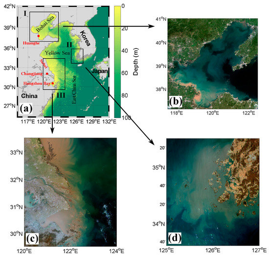
Figure 1.
(a) Bathymetry for the Bohai Sea, Yellow Sea, and East China Sea. Three highly turbid water areas are outlined in three boxes (I, II, and III). Panels (b–d) are the composed RGB pictures of the three examples used for comparison (B: 490 nm, G: 555 nm, and R: 680 nm).
The Bohai Sea is a shallow semi-enclosed sea with an average water depth of 18 m and a maximum depth of ~70 m. It deepens gradually from the coastal bays to the Central Bohai Sea and is characterized by a basin shape [20]. The dominant sediment source in this region is the sediment delivered by the Huanghe [21,22]. The high suspended sediment concentration is mainly distributed in the south of Bohai Sea, especially in the area around the Huanghe Delta [21].
The water depth of the area along the Southwestern Korean coast is less than 50 m. Numerous islands and vast tidal flats are located here and the coastlines in this area are complicated. The suspended sediment concentration of this area is relatively high (>20 g/m3). The highest values (>100 g/m3) occur in the winter owing to the stronger northwestern monsoon and shallow water depth, which can induce a resuspension of bottom sediments [23].
The Changjiang Estuary is located along the central-eastern coast of China, with the Hangzhou Bay to the south and the Subei Shallow to the north. The highly suspended sediment concentrations were observed here year-round [24]. The Changjiang River discharges about 390 × 106 tons of sediment into the East China Sea annually [25]. The sediment transportation inside the Hangzhou Bay is considerably affected by the secondary Changjiang plume [26]. Another major sediment source for the East China Sea is the resuspension of sediment at the Subei Shallow [27]. Wind-induced vertical mixing and bottom stress tend to resuspend a large amount of sediment, leading to high suspended sediment concentrations, especially in the winter [28,29].
One cloud-free example is chosen from each of these regions. The RGB pictures of the three examples are composed of the total radiance at 490 nm (B), 555 nm (G), and 680 nm (R) bands of GOCI and are shown in Figure 1b–d. More details of the three examples are listed in Table 1.

Table 1.
Detail information on the processed images.
3. Method
Reflectance ρ is defined as:
where λ denotes the wavelength, F0 is the extraterrestrial solar irradiance [30], θs is the solar zenith angle, and L is the radiance. It is more convenient to work with ρ because it is dimensionless. The total reflectance ρt(λ) measured by a sensor can be written as:
where ρr denotes Rayleigh scattering reflectance, ρa denotes aerosol multiple scattering reflectance, ρw denotes water-leaving reflectance, and tv denotes the Rayleigh–aerosol diffuse transmittance from the sea surface to the satellite. It should be noted that the reflectance contributions from the sun glint and whitecaps are ignored [31,32].
Determining the remote sensing reflectance (Rrs, unit: sr−1) and normalized water-leaving reflectance (ρwn) is the ultimate goal of AC because they are fundamental parameters that are widely used for deriving the water constituent concentrations and water quality parameters. These can be calculated by:
where ts is the diffuse transmittance from the sun to the sea surface.
In this section, we briefly review the previous AC algorithms that were adopted in the main GOCI processing software: SeaDAS (SeaWiFS Data Analysis System) and GDPS (GOCI data process system). Then, the development of the new algorithm is described.
3.1. Previous AC Algorithms
The key problem of AC over turbid waters is the removal of the water-leaving reflectance at NIR bands. Numerous red/NIR modeling approaches have been investigated to deal with non-zero ρw(red/NIR) values within the AC process. Three kinds of AC approaches are briefly reviewed herein—the B2010 AC algorithm proposed by Bailey et al. [33] is currently adopted in SeaDAS, while the A2012 algorithm proposed by Ahn et al. [34] and the L2013 algorithm proposed by Lee et al. [35] are implemented in GDPS.
The B2010 algorithm uses an iterative solution to separate ρw(NIR) and ρa(NIR). The ρw(NIR) is first assumed to be zero to complete the GW94 AC process. This gives an initial estimate of Rrs(λ). Next, the concentration of chlorophyll-a is preliminarily estimated by the initial value of Rrs(λ). Then, the absorption coefficient in the red band is obtained via a chlorophyll-a–based empirical relationship. The absorption coefficient and Rrs in the red band are used to solve the backscattering coefficient, which is used to extrapolate the ρw at the NIR band. Finally, the new values of ρw(NIR) are used to correct the non-zero water contribution, and the GW94 AC step is repeated for a new iteration.
The A2012 algorithm is the GOCI standard AC algorithm. It is theoretically based on the GW94 algorithm with partial modifications. The initial ρw(NIR) values are also assumed to be zero to execute the GW94 algorithm. The newly estimated ρwn in the red band is used to correct the ρwn(NIR) by an empirical polynomial relationship model [36]:
where jn and kn are known polynomial coefficients.
The L2013 algorithm is from the Management Unit of the North Sea Mathematical Models (MUMM) [37] algorithm, with some modified steps for extremely turbid water. In the original MUMM, the parameter α, representing the ratio of ρw at the NIR wavelengths, is assumed to have spatial homogeneity; however, the value of α changes with the concentration of suspended particles in extremely turbid waters, which would cause an underestimation of the water-leaving radiances [38]. The L2013 algorithm calculates the α value adaptively using an NIR water-leaving reflectance model:
where the cn values are known polynomial coefficients.
The algorithms mentioned above can improve the data quality in turbid waters, but the empirical relationships are highly reliant on in situ datasets; even the empirical relationship used in L2013 is derived from the nearest non-turbid AC algorithm [39]. These algorithms are, therefore, only regionally applicable [40]. For example, the B2010 method only works properly in low to moderately turbid waters [41,42], as the chlorophyll-a–based relationship used in the bio-optical model might not be appropriate to extrapolate the ρw(NIR) in waters whose optical properties are dominated by non-algal particles [41,42]. The A2012 method is suitable for sediment-dominated waters but also fails for extremely turbid waters because the ρwn(660 nm) can become optically saturated [43].
3.2. The Development of the New AC Algorithm
In order to distinguish the two sensors, the superscripts V and G represent VIIRS and GOCI, respectively. The procedure for the new algorithm can be divided into four parts:
- Extracting the ρa(NIRV) of VIIRS;
- Estimating the aerosol properties by ρa(NIRV);
- Calculating the ρa(λG) at GOCI observing geometries according to the aerosol properties; and
- Removing the ρa(λG) and completing the GOCI AC process.
The removal of the ρw(NIRV) of VIIRS follows the Shortwave Infrared Exponential (SWIRE) algorithm [12], in which the Rayleigh-corrected reflectance values ρrc (ρrc = ρt − ρr) of clear waters were assumed to be an exponential function of wavelength at the NIR/SWIR bands:
where ρef is the extrapolated Rayleigh-corrected reflectance, and a and b are the fitting coefficients.
The ρrc values at the three VIIRS SWIR bands (1238, 1601, and 2257 nm) are used to calculate the coefficients a and b because the ρrc at the NIR bands is strongly influenced by suspended sediments scattering in turbid waters. The newly estimated ρef(NIR) can be considered to be the ρrc of the optical equivalent clear water, influenced only by aerosol scattering, and can be used for the GW94 AC of the visible bands. The SWIR-based methods improve the ocean color products in the turbid coastal waters, but they require higher signal-to-noise ratios (SNR) for SWIR bands because of the longer extrapolated distances and lower signals [44]. Wang and Shi [14] used two SWIR bands to derive the aerosol scattering radiance, but their method did not achieve better results than the NIR-based methods in non-turbid waters because significant noise occurred in the derived products [45,46]. Generally, the more SWIR bands used, the more accurately can the aerosol scattering reflectance be estimated, and the requirements of SNR can probably be reduced. As a result, the SWIRE method represented an improvement over the SWIR-based methods [47].
The newly estimated ρef(NIRV) can be considered as the ρa(NIRV) and can be applied to evaluate the aerosol properties of the observing area, including the contributing aerosol models and aerosol optical thickness τa. The contributing aerosol models are selected by the look-up-tables (LUTs) for 80 aerosol tables constructed by Ahmad et al. [48]. The parameters used to derive the aerosol single-scattering albedo (ωa), aerosol scattering phase function (Pa), and extinction coefficient (βa) are stored in the LUTs for each aerosol model and various geometries. The LUTs also contain the coefficients relating single to multiple scattering and the coefficients (A and B) used to calculate the Rayleigh–aerosol, diffuse transmittance in the following form [49]:
The aerosol optical thickness is the normalized extinction coefficient due to absorption and scattering from the direct beam and is a key parameter used to define the optical state of the atmosphere [50,51].
The estimation of the aerosol properties follows the GW94 method [4], which is one of the AC algorithms widely used for clear waters. In this algorithm, ρa(NIRV) is first converted into ρas(NIRV) [52] by solving the quadratic equation:
where the pn values are the quadratic coefficients stored in the LUTs. The AC parameter is defined as:
where NIRS is the short-wavelength NIR band, and NIRL is the long-wavelength NIR band. For the VIIRS sensor, the NIRS and NIRL are 745 nm and 862 nm, respectively. Theoretically, each candidate aerosol model has its own ε value (εM) for a specific geometry:
Two aerosol models with different weighting factors whose ε(NIRS, NIRL) values are the closest to the εM(NIRS, NIRL) averaged over all candidate models, are chosen to represent the aerosol type over the pixel. The selection of the closest aerosol models can dominate the estimation of the water-leaving reflectance, especially over turbid coastal waters [53]. The τa(745 nm) values of the two contributing models can be retrieved by [4]:
The VIIRS sensor is located in a sun-synchronous orbit and provides one image per day, whereas the GOCI sensor is located in a geostationary orbit and provides eight images per day. With the hourly observations from the GOCI, the VIIRS image has a corresponding GOCI image with a time difference of less than half an hour, which means the atmospheric conditions are nearly invariant. Therefore, the aerosol scattering reflectance of the GOCI observing geometries can be derived according to the known contributing aerosol models, weighting factor, and the τa(745 nm). First, calculate the τa(λG) of each contributing aerosol model by:
Second, calculate the ρas(λG) by Equation (13). Next, convert ρas(λG) to ρam(λG) via Equation (10). Finally, the effects of the two contributing aerosol models are superimposed by weighting factors to estimate the total aerosol scattering reflectance of GOCI. In order to maintain the higher spatial resolution of GOCI, the aerosol parameters estimated from VIIRS are resampled to the GOCI data grid by the nearest neighbor method.
4. Results and Discussion
In the absence of in situ data, the results of the new algorithm (represented by QSV) are compared with those processed by the B2010 [33], A2012 [34], and L2013 [35] algorithms. VIIRS and GOCI Level-1 data were obtained online (https://oceancolor.gsfc.nasa.gov). For the QSV algorithm, the Rayleigh-corrected reflectance values were obtained by using the SeaDAS 7.4 l2gen processor, and these values were used as the inputs of the aerosol scattering correction procedure, which was performed by using Interactive Data Language (IDL). With default settings, the B2010 algorithm was realized by the SeaDAS 7.4 software, while the A2012 and L2013 algorithms were realized by the GDPS v1.4.1 software. The three examples listed in Table 1 are processed.
Figure 2, Figure 3 and Figure 4 represent the Rrs values retrieved by four different algorithms centered at the Bohai Sea, the southwest coast of Korea, and the Changjiang Estuary, respectively. Panels (a–d), (e–h), and (i–l) are results at wavelengths of 490, 555, and 680 nm, respectively. The regions in which the algorithms fail to make an AC because of highly turbid waters or due to the presence of clouds and land, are shown with RGB pictures. It can be observed that the Rrs distributions are similar for all four algorithms, but the B2010, A2012, and L2013 algorithms result in varying degrees of failures, while the QSV algorithm can successfully execute the AC in the highly turbid coastal waters. The unmasked abnormal low estimations from L2013 also can be observed at 35°N, 126°E in Figure 3b,f,j, highlighted by the red circles.

Figure 2.
Comparisons of the Rrs distributions (unit: sr−1) at (a–d) 490, (e–h) 555, and (i–l) 680 nm bands centered on the Bohai Sea on 26 August 2016 and processed by the B2010, L2013, A2012, and QSV algorithms. The regions in which the algorithms fail to make an AC because of highly turbid waters, or the presence of clouds and land are shown by the composed RGB pictures (B: 490 nm, G: 555 nm, R: 680 nm).

Figure 3.
Comparisons of the Rrs distributions (unit: sr−1) at the (a–d) 490, (e–h) 555, and (i–l) 680 nm bands centered on the southwest coast of Korea on 14 March 2017 and processed by the B2010, L2013, A2012, and QSV algorithms. The regions in which the algorithms fail to make an AC because of highly turbid waters, or the presence of clouds and land are shown by the composed RGB pictures (B: 490 nm, G: 555 nm, and R: 680 nm). The unmasked abnormal low estimations from L2013 are highlighted by the red circles in panels (b,f,j).

Figure 4.
Comparisons of the Rrs distributions (unit: sr−1) at (a–d) 490, (e–h) 555, and (i–l) 680 nm bands centered on the Changjiang Estuary on 1 March 2016 and processed by the B2010, L2013, A2012, and QSV algorithms. The red arrow in panel (a) refers to the location and direction of the transect used in Figure 5. The regions in which the algorithms fail to make an AC because of highly turbid waters, or the presence of clouds and land are shown by the composed RGB pictures (B: 490 nm, G: 555 nm, and R: 680 nm).
To further demonstrate the differences, we also extracted the Rrs(λ) values for pixels along the red arrow in Figure 4a and plotted their profiles in Figure 5. A distance of 0 along the x-axis indicates the location closest to the coast. In general, the Rrs data are low in the open ocean and high near the coast. The mean absolute difference in the Rrs values between the A2012 and QSV algorithms is the smallest, with values of 0.00334, 0.00138, 0.00100, 0.00091, 0.00110, and 0.00182 sr−1 at wavelengths of 412, 443, 490, 555, 660, and 680 nm, respectively. At around 0 to 110 pixels along the transect, the B2010 algorithm is invalid. The results of the L2013 are relatively higher than those of the A2012 and QSV algorithms, at distances larger than 50 pixels along the transect. Abnormal fluctuations of the L2013 curves can be observed at around 25–50 pixels. The A2012 and L2013 methods both fail at around 0–25 pixels. The QSV is the only algorithm that can retrieve continuous and reasonable values of Rrs along the total transect.
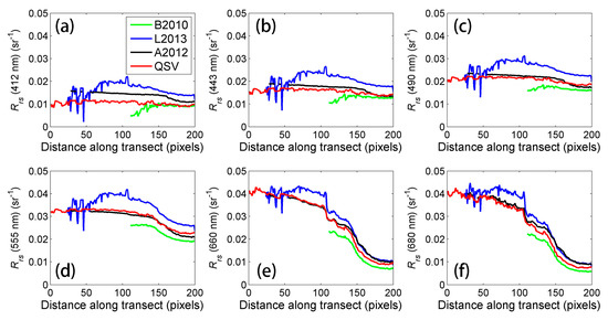
Figure 5.
Comparison of the Rrs values extracted from the pixels along the red arrow in Figure 4a at wavelengths of (a) 412, (b) 443, (c) 490, (d) 555, (e) 660, and (f) 680 nm. A distance of 0 in the x-axis indicates the location closest to the coast.
Three sets of Rrs spectra derived from four different AC algorithms in highly turbid waters at station (a), moderately turbid water at station (b), and clear water at station (c) are compared and shown in Figure 6. At station (c), the curves of the B2010, A2012, and QSV algorithms tend to be coincident, while the Rrs values retrieved by L2013 are relatively high. At station (b), the B2010 algorithm shows slightly lower estimations. At station (a), the B2010 algorithm has no valid results, and the difference between L2013 and A2012/QSV is more pronounced.

Figure 6.
Comparisons of the Rrs spectra derived from four different algorithms in highly turbid waters at station (a), moderately turbid waters at station (b), and clear waters at station (c). The RGB image shows the locations of the three stations.
Since these four algorithms are developed for turbid waters, they can all improve the data quality in turbid waters. The B2010, A2012, and L2013 algorithms are based on empirical models and are highly regionally dependent. Significant errors or failures can be induced when these methods are applied to the ocean regions they are not suitable for. Even though the QSV algorithm can be applied to only one scene of the GOCI data, it can obtain reasonable results in extremely turbid coastal waters. The use of three SWIR bands can improve the data quality of the AC retrievals in clear waters without obvious noise. In general, the QSV algorithm provides a simple, effective, new AC approach for GOCI to obtain reasonable results in highly turbid waters and provides an alternative method to validating other AC methods.
5. Conclusions
An alternative AC algorithm using quasi-synchronous VIIRS data for GOCI in highly turbid waters is presented in this paper. GOCI covers highly turbid waters in the Western Pacific region; AC has been a challenge in these turbid ocean regions because of the lack of SWIR bands. The new algorithm shows its superiority in highly turbid coastal waters, and the results could be at least be used for the validation of other AC methods. However, there are still some limitations that should be noted. The major disadvantage of this algorithm is that only one VIIRS image per day is not sufficient for GOCI, and more in situ data are needed for the validation. In the future, GOCI-2 will have full-disk coverage with higher resolution and five more bands than GOCI does, but it will still not have any SWIR bands [54]. Including SWIR bands on a sensor is expensive, therefore, further research is necessary on how to best take advantage of SWIR bands from other ocean color sensors.
Author Contributions
Conceptualization, C.C. and J.W.; implementation, C.C. and J.W.; validation, J.W. and S.N.; writing-original draft preparation, J.W. and S.N.; writing-review and editing, C.C., J.W., and S.N.; funding acquisition: C.C. All authors have read and agreed to the published version of the manuscript.
Funding
This research was funded by the National Natural Science Foundation of China [grant number U1901215], the National Key Research and Development Projects [grant number 2018YFC1406604], the Scientific Research Key Project from Guangzhou City [grant number 201707020031], the National Natural Science Foundation of China [grant number 41276182], and the Project of State Key Laboratory of Tropical Oceanography [grant number LTOZZ1705].
Acknowledgments
We wish to thank NASA’s Ocean Biology Processing Group (OBPG) for providing the SeaDAS software package and VIIRS/SNPP Level 1-A data. We also wish to thank the Korea Ocean Satellite Center for providing the GDPS software package and GOCI Level-1 data.
Conflicts of Interest
The authors declare no conflict of interest.
References
- Wang, M.H. A sensitivity study of the SeaWiFS atmospheric correction algorithm: Effects of spectral band variations. Remote Sens. Environ. 1999, 67, 348–359. [Google Scholar] [CrossRef]
- Wang, M.H. A refinement for the Rayleigh radiance computation with variation of the atmospheric pressure. Int. J. Remote Sens. 2005, 26, 5651–5663. [Google Scholar] [CrossRef]
- Wang, M.H. Rayleigh radiance computations for satellite remote sensing: Accounting for the effect of sensor spectral response function. Opt. Express 2016, 24, 2414–2429. [Google Scholar] [CrossRef] [PubMed]
- Gordon, H.R.; Wang, M. Retrieval of water-leaving radiance and aerosol optical thickness over the oceans with SeaWiFS: A preliminary algorithm. Appl. Opt. 1994, 33, 443–452. [Google Scholar] [CrossRef] [PubMed]
- Emberton, S.; Chittka, L.; Cavallaro, A.; Wang, M.H. Sensor Capability and Atmospheric Correction in Ocean Colour Remote Sensing. Remote Sens. 2016, 8, 1. [Google Scholar] [CrossRef]
- Ryu, J.H.; Han, H.J.; Cho, S.; Park, Y.J.; Ahn, Y.H. Overview of Geostationary Ocean Color Imager (GOCI) and GOCI Data Processing System (GDPS). Ocean Sci. J. 2012, 47, 223–233. [Google Scholar] [CrossRef]
- Hu, Z.F.; Pan, D.L.; He, X.Q.; Bai, Y. Diurnal Variability of Turbidity Fronts Observed by Geostationary Satellite Ocean Color Remote Sensing. Remote Sens. 2016, 8, 147. [Google Scholar] [CrossRef]
- Choi, J.K.; Min, J.E.; Noh, J.H.; Han, T.H.; Yoon, S.; Park, Y.J.; Moon, J.E.; Ahn, J.H.; Ahn, S.M.; Park, J.H. Harmful algal bloom (HAB) in the East Sea identified by the Geostationary Ocean Color Imager (GOCI). Harmful Algae 2014, 39, 295–302. [Google Scholar] [CrossRef]
- Liu, R.J.; Zhang, J.; Yao, H.Y.; Cui, T.W.; Wang, N.; Zhang, Y.; Wu, L.J.; An, J.B. Hourly changes in sea surface salinity in coastal waters recorded by Geostationary Ocean Color Imager. Estuar Coast Shelf Sci. 2017, 196, 227–236. [Google Scholar] [CrossRef]
- Choi, J.K.; Park, Y.J.; Ahn, J.H.; Lim, H.S.; Eom, J.; Ryu, J.H. GOCI, the world’s first geostationary ocean color observation satellite, for the monitoring of temporal variability in coastal water turbidity. J. Geophys. Res. Ocean. 2012, 117. [Google Scholar] [CrossRef]
- Vanhellemont, Q.; Ruddick, K. Advantages of high quality SWIR bands for ocean colour processing: Examples from Landsat-8. Remote Sens. Environ. 2015, 161, 89–106. [Google Scholar] [CrossRef]
- He, Q.J.; Chen, C.Q. A new approach for atmospheric correction of MODIS imagery in turbid coastal waters: A case study for the Pearl River Estuary. Remote Sens. Lett. 2014, 5, 249–257. [Google Scholar] [CrossRef]
- Wang, M.H.; Shi, W. Estimation of ocean contribution at the MODIS near-infrared wavelengths along the east coast of the US: Two case studies. Geophys. Res. Lett. 2005, 32. [Google Scholar] [CrossRef]
- Wang, M.H.; Shi, W. The NIR-SWIR combined atmospheric correction approach for MODIS ocean color data processing. Opt. Express 2007, 15, 15722–15733. [Google Scholar] [CrossRef] [PubMed]
- Jiang, L.D.; Wang, M.H. Improved near-infrared ocean reflectance correction algorithm for satellite ocean color data processing. Opt. Express 2014, 22, 21657–21678. [Google Scholar] [CrossRef]
- Cao, C.Y.; de Luccia, F.J.; Xiong, X.X.; Wolfe, R.; Weng, F.Z. Early On-Orbit Performance of the Visible Infrared Imaging Radiometer Suite Onboard the Suomi National Polar-Orbiting Partnership (S-NPP) Satellite. IEEE Trans. Geosci. Remote 2014, 52, 1142–1156. [Google Scholar] [CrossRef]
- Shi, W.; Zhang, Y.L.; Wang, M.H. Deriving Total Suspended Matter Concentration from the Near-Infrared-Based Inherent Optical Properties over Turbid Waters: A Case Study in Lake Taihu. Remote Sens. 2018, 10, 333. [Google Scholar] [CrossRef]
- Cao, C.Y.; Xiong, J.; Blonski, S.; Liu, Q.H.; Uprety, S.; Shao, X.; Bai, Y.; Weng, F.Z. Suomi NPP VIIRS sensor data record verification, validation, and long-term performance monitoring. J. Geophys. Res. Atmos. 2013, 118, 11664–11678. [Google Scholar] [CrossRef]
- Wang, M.H.; Son, S. VIIRS-derived chlorophyll-a using the ocean color index method. Remote Sens. Environ. 2016, 182, 141–149. [Google Scholar] [CrossRef]
- Bian, C.W.; Jiang, W.S.; Pohlmann, T.; Sundermann, J. Hydrography-Physical Description of the Bohai Sea. J. Coast. Res. 2016, 74, 1–12. [Google Scholar] [CrossRef]
- Wang, H.J.; Wang, A.M.; Bi, N.H.; Zeng, X.M.; Xiao, H.H. Seasonal distribution of suspended sediment in the Bohai Sea, China. Cont. Shelf Res. 2014, 90, 17–32. [Google Scholar] [CrossRef]
- Milliman, J.D.; Li, F.; Zhao, Y.Y.; Zheng, T.M.; Limeburner, R. Suspended Matter Regime in the Yellow Sea. Prog. Oceanogr. 1986, 17, 215–227. [Google Scholar] [CrossRef]
- Min, J.E.; Choi, J.K.; Yang, H.; Lee, S.; Ryu, J.H. Monitoring changes in suspended sediment concentration on the southwestern coast of Korea. J. Coast. Res. 2014, 133–138. [Google Scholar] [CrossRef]
- Dong, L.X.; Guan, W.B.; Chen, Q.; Li, X.H.; Liu, X.H.; Zeng, X.M. Sediment transport in the Yellow Sea and East China Sea. Estuar. Coast. Shelf Sci. 2011, 93, 248–258. [Google Scholar] [CrossRef]
- Wang, Y.; Shen, J.; He, Q.; Zhu, L.; Zhang, D. Seasonal variations of transport time of freshwater exchanges between Changjiang Estuary and its adjacent regions. Estuar. Coast. Shelf Sci. 2015, 157, 109–119. [Google Scholar] [CrossRef]
- Su, J.L.; Wang, K.S. Changjiang River Plume and Suspended Sediment Transport in Hangzhou Bay. Cont. Shelf Res. 1989, 9, 93–111. [Google Scholar]
- Saito, Y.; Yang, Z.S. Historical change of the Huanghe (Yellow River) and its impact on the sediment budget of the East China Sea. In Global Fluxs of Carbon and Its Related Substances in the Coastal Sea-Ocean Atmosphere System; M & J International: Yokohama, Japan, 1995. [Google Scholar]
- Bian, C.W.; Jiang, W.S.; Quan, Q.; Wang, T.; Greatbatch, R.J.; Li, W. Distributions of suspended sediment concentration in the Yellow Sea and the East China Sea based on field surveys during the four seasons of 2011. J. Mar. Syst. 2013, 121, 24–35. [Google Scholar] [CrossRef]
- Bian, C.W.; Jiang, W.S.; Greatbatch, R.J. An exploratory model study of sediment transport sources and deposits in the Bohai Sea, Yellow Sea, and East China Sea. J. Geophys. Res. Ocean. 2013, 118, 5908–5923. [Google Scholar] [CrossRef]
- Thuillier, G.; Herse, M.; Simon, P.C.; Labs, D.; Mandel, H.; Gillotay, D.; Foujols, T. The visible solar spectral irradiance from 350 to 850 nm as measured by the SOLSPEC spectrometer during the ATLAS I mission. Sol. Phys. 1998, 177, 41–61. [Google Scholar] [CrossRef]
- Gordon, H.R.; Wang, M.H. Influence of Oceanic Whitecaps on Atmospheric Correction of Ocean-Color Sensors. Appl. Opt. 1994, 33, 7754–7763. [Google Scholar] [CrossRef]
- Wang, M.H.; Bailey, S.W. Correction of sun glint contamination on the SeaWiFS ocean and atmosphere products. Appl. Opt. 2001, 40, 4790–4798. [Google Scholar] [CrossRef]
- Bailey, S.W.; Franz, B.A.; Werdell, P.J. Estimation of near-infrared water-leaving reflectance for satellite ocean color data processing. Opt. Express 2010, 18, 7521–7527. [Google Scholar] [CrossRef] [PubMed]
- Ahn, J.H.; Park, Y.J.; Ryu, J.H.; Lee, B.; Oh, I.S. Development of Atmospheric Correction Algorithm for Geostationary Ocean Color Imager (GOCI). Ocean Sci. J. 2012, 47, 247–259. [Google Scholar] [CrossRef]
- Lee, B.; Ahn, J.H.; Park, Y.J.; Kim, S.W. Turbid water atmospheric correction for GOCI: Modification of MUMM algorithm. Korean J. Remote Sens. 2013, 29, 173–182. [Google Scholar] [CrossRef]
- Park, Y.J.; Ahn, Y.H.; Han, H.J.; Yang, H.; Moon, J.E.; Ahn, J.H.; Lee, B.R.; Min, J.E.; Lee, S.J.; Kim, K.S.; et al. GOCI Level 2 Ocean Color Products (GDPS 1.3) Brief Algorithm Description; Korea Ocean Satellite Center, Korea Institute of Ocean Science and Technology: Ansan, Korea, 2014. [Google Scholar]
- Ruddick, K.G.; Ovidio, F.; Rijkeboer, M. Atmospheric correction of SeaWiFS imagery for turbid coastal and inland waters. Appl. Opt. 2000, 39, 897–912. [Google Scholar] [CrossRef] [PubMed]
- Goyens, C.; Jamet, C.; Schroeder, T. Evaluation of four atmospheric correction algorithms for MODIS-Aqua images over contrasted coastal waters. Remote Sens. Environ. 2013, 131, 63–75. [Google Scholar] [CrossRef]
- Hu, C.M.; Carder, K.L.; Muller-Karger, F.E. Atmospheric correction of SeaWiFS imagery over turbid coastal waters: A practical method. Remote Sens. Environ. 2000, 74, 195–206. [Google Scholar] [CrossRef]
- Huang, X.C.; Zhu, J.H.; Han, B.; Jamet, C.; Tian, Z.; Zhao, Y.L.; Li, J.; Li, T.J. Evaluation of Four Atmospheric Correction Algorithms for GOCI Images over the Yellow Sea. Remote Sens. 2019, 11, 1631. [Google Scholar] [CrossRef]
- Goyens, C.; Jamet, C.; Ruddick, K.G. Spectral relationships for atmospheric correction. II. Improving NASA’s standard and MUMM near infra-red modeling schemes. Opt. Express 2013, 21, 21176–21187. [Google Scholar] [CrossRef]
- Goyens, C.; Jamet, C.; Ruddick, K.G. Spectral relationships for atmospheric correction. I. Validation of red and near infra-red marine reflectance relationships. Opt. Express 2013, 21, 21162–21175. [Google Scholar] [CrossRef]
- Doxaran, D.; Froidefond, J.M.; Lavender, S.; Castaing, P. Spectral signature of highly turbid waters—Application with SPOT data to quantify suspended particulate matter concentrations. Remote Sens. Environ. 2002, 81, 149–161. [Google Scholar] [CrossRef]
- Wang, M.H.; Son, S.; Shi, W. Evaluation of MODIS SWIR and NIR-SWIR atmospheric correction algorithms using SeaBASS data. Remote Sens. Environ. 2009, 113, 635–644. [Google Scholar] [CrossRef]
- Wang, M.H.; Shi, W. Sensor Noise Effects of the SWIR Bands on MODIS-Derived Ocean Color Products. IEEE Trans. Geosci. Remote 2012, 50, 3280–3292. [Google Scholar] [CrossRef]
- Carswell, T.; Costa, M.; Young, E.; Komick, N.; Gower, J.; Sweeting, R. Evaluation of MODIS-Aqua Atmospheric Correction and Chlorophyll Products of Western North American Coastal Waters Based on 13 Years of Data. Remote Sens. 2017, 9, 1063. [Google Scholar] [CrossRef]
- Ye, H.B.; Chen, C.Q.; Yang, C.Y. Atmospheric Correction of Landsat-8/OLI Imagery in Turbid Estuarine Waters: A Case Study for the Pearl River Estuary. IEEE J. STARS 2017, 10, 252–261. [Google Scholar] [CrossRef]
- Ahmad, Z.; Franz, B.A.; McClain, C.R.; Kwiatkowska, E.J.; Werdell, J.; Shettle, E.P.; Holben, B.N. New aerosol models for the retrieval of aerosol optical thickness and normalized water-leaving radiances from the SeaWiFS and MODIS sensors over coastal regions and open oceans. Appl. Opt. 2010, 49, 5545–5560. [Google Scholar] [CrossRef]
- Yang, H.Y.; Gordon, H.R. Remote sensing of ocean color: Assessment of water-leaving radiance bidirectional effects on atmospheric diffuse transmittance. Appl. Opt. 1997, 36, 7887–7897. [Google Scholar] [CrossRef]
- Masmoudi, M.; Chaabane, M.; Tanre, D.; Gouloup, P.; Blarel, L.; Elleuch, F. Spatial and temporal variability of aerosol: Size distribution and optical properties. Atmos. Res. 2003, 66, 1–19. [Google Scholar] [CrossRef]
- Queface, A.J.; Piketh, S.J.; Annegarn, H.J.; Holben, B.N.; Uthui, R.J. Retrieval of aerosol optical thickness and size distribution from the CIMEL Sun photometer over Inhaca Island, Mozambique. J. Geophys. Res. Atmos. 2003, 108. [Google Scholar] [CrossRef]
- Franz, B.A. rhoa_to_rhoas—MS aerosol reflectance to SS aerosol reflectance. In Aerosol.c in SeaDAS Code; NASA’s Ocean Biology Processing Group (OBPG), 2004. Available online: http://seadas.gsfc.nasa.gov (accessed on 8 January 2016).
- McCarthy, S.C.; Gould, R.W.; Richman, J.; Kearney, C.; Lawson, A. Impact of Aerosol Model Selection on Water-Leaving Radiance Retrievals from Satellite Ocean Color Imagery. Remote Sens. 2012, 4, 3638–3665. [Google Scholar] [CrossRef]
- Cho, S. Introduction of GOCI and GOCI-II Mission with Lunar Calibration. In Lunar Calibration Workshop; EUMETSAT: Darmstadt, Germany; Available online: http://gsics.atmos.umd.edu/pub/Development/ LunarCalibrationWorkshop/4b_Cho_GOCI2.pdf (accessed on 10 August 2018).


© 2019 by the authors. Licensee MDPI, Basel, Switzerland. This article is an open access article distributed under the terms and conditions of the Creative Commons Attribution (CC BY) license (http://creativecommons.org/licenses/by/4.0/).