Article

Bayesian Harmonic Modelling of Sparse and Irregular Satellite Remote Sensing Time Series of Vegetation Indexes: A Story of Clouds and Fires

by
Saverio Vicario
1,*,
Maria Adamo
1,
Domingo Alcaraz-Segura
2,3 and
Cristina Tarantino
1
1
Institute of Atmospheric Pollution Research–Italian National Research Council C/O Department of Physics, University of Bari, via Orabona 4, 70125 Bari, Italy
2
Department of Botany and Inter-University Institute for Earth System Research (IISTA), University of Granada, 18071 Granada, Spain
3
Andalusian Center for the Assessment and Monitoring of Global Change (CAESCG), University of Almería, 04120 Almería, Spain
*
Author to whom correspondence should be addressed.
Remote Sens. 2020, 12(1), 83; https://doi.org/10.3390/rs12010083
Submission received: 6 November 2019 / Revised: 6 December 2019 / Accepted: 17 December 2019 / Published: 24 December 2019
(This article belongs to the Special Issue Remote Sensing in Ecosystem Modelling)

Abstract

:
Vegetation index time series from Landsat and Sentinel-2 have great potential for following the dynamics of ecosystems and are the key to develop essential variables in the realm of biodiversity. Unfortunately, the removal of pixels covered mainly by clouds reduces the temporal resolution, producing irregularity in time series of satellite images. We propose a Bayesian approach based on a harmonic model, fitted on an annual base. To deal with data sparsity, we introduce hierarchical prior distribution that integrate information across the years. From the model, the mean and standard deviation of yearly Ecosystem Functional Attributes (i.e., mean, standard deviation, and peak’s day) plus the inter-year standard deviation are calculated. Accuracy is evaluated with a simulation that uses real cloud patterns found in the Peneda-Gêres National Park, Portugal. Sensitivity to the model’s abrupt change is evaluated against a record of multiple forest fires in the Bosco Difesa Grande Regional Park in Italy and in comparison with the BFAST software output. We evaluated the sensitivity in dealing with mixed patch of land cover by comparing yearly statistics from Landsat at 30m resolution, with a 2m resolution land cover of Murgia Alta National Park (Italy) using FAO Land Cover Classification System 2.

1. Introduction

The primary productivity of plants is an essential variable both for the biodiversity (as a driver of the ecosystem’s carrying capacity) and climate (as a driver of evapotranspiration, as well as being directly involved in carbon fixation). In situ measurements of Gross Primary Productivity (GPP) require large and costly infrastructures to estimate the CO2 fluxes from an eddy covariance measurement of net ecosystems exchange.
Satellite data is used to obtain measurements on a large temporal and spatial scale. However, as the signal is highly disturbed by the atmosphere, even the comparison among surface reflectance values (i.e., atmospherically corrected) from the same geographical location across different images entails multiple sources of errors. Fortunately, the error is nearly unbiased [1] and has a normal probability distribution, probably caused by the multiple effect of small source of errors (i.e., in the atmosphere correction, in pixel geometry, etc.).
Several tools were developed to both correct noise from the time series of satellite data and to build robust summary statistics based on seasonality and changes, generally by partitioning values in a seasonal component and a trend component [2]. Different nonparametric and parametric approaches are considered in literature. Within a nonparametric approach, is possible to use climatological statistics where, selecting a yearly time-partitioning (i.e., day, month, and season), the mean value is estimated across the years to define a seasonal expectation. Deviation from expectation is subsequently analysed with a moving average or a trend line in order to extract the long term change, whereas residuals are considered as noise [2,3]. Another nonparametric approach is based on fast Fourier transform called Singular Spectrum Analysis [2,4], whereas the spectral analysis is used to estimate the seasonal component. Within the parametric approaches, the most common methods are based on a harmonic model where a linear regression with a sinusoidal predictor and a trend predictor are used to decompose the time series signal. The oldest implementation of Harmonic ANalysis of Time Series (HANTS) ([5,6] focused on the Top of Atmosphere signal with fixed seasonality and trend. A more recent implementation as Breaks For Additive Season and Trend (BFAST) [7], allows changes both within seasonal and trend components. Finally, noticing that some seasonal statistics are difficult to estimate with few harmonics in case of abrupt seasonal changes, such as the start of the growing season at higher latitudes, Timesat [8] also added, beside harmonic model, a symmetric Gaussian and double logistic model to the tool-kit. Both new models are nonlinear and the user needs to explicitly decide how many growing seasons will need to be considered. All these tools assume that the time series need to have regularly spaced information and have limited or no capacity to handle missing data. This regularity assumption apparently seems reasonable, given that satellites feature a highly regular passing time. However, in case of localities with a seasonal cloud cover, this assumption does not hold. In nonparametric approaches, irregularities of sampling cause noise that overcomes the signal [3]. Often, to fulfil the regularity assumption, which is essential for the cited parametric approaches, data are interpolated using a filtering procedure such as Savitzky–Golay. Nevertheless, the risk is not only to alter the true signal in case of missing data covering a key moment of one or more growing seasons, but also to alter the error estimation and therefore to inflate the confidence in the results given. The free available time series from Landsat and Sentinel-2 satellites are often irregular due to low-quality filtering due to the presences of clouds, shadows and aerosols. In some locations they are very sparse, with less than 10 unevenly-spaced observations per year (e.g., in the Peneda-Gerês National Park in Portugal). This is a very typical situation in cloudy regions, such as in the tropics and high latitudes, where few yearly observations are usually available [9].
To overcome the limit of pairing non parametric interpolation followed by parametric seasonal statistics estimation, it is necessary to build tools for time series analysis that are able to handle sparse and uneven data. In this article, we propose a new method to remove noise and produce seasonal statistics from time series of satellite images of vegetation indices. As a general approach, we selected harmonic models that are intrinsically more flexible to handle time series with a different number of growing seasons per year (typical in the Mediterranean biome [10]). To test the effectiveness of the method, we assessed its effect on the key descriptors of the seasonal cycle of vegetation indices, i.e., Ecosystem Functional Attributes (EFA) as a set of essential variables that synthesize seasonality variations [11], which are flexible enough to be applied in different regions worldwide.

2. Materials

2.1. Study Areas

Three sites were selected in order to evaluate the proposed approach (Figure 1). First, we selected the Peneda Gerês National Park, because it presents an intense permanent cloud cover and indeed the need to analyse this region is the initial reason why this method was developed. The region is characterized by mid-altitude mountains with peaks of less that 1600 m above mean sea level that constitute a barrier for the clouds between plain of Northern Portugal over the ocean and the continental Spanish plain. The cloud pattern of this region was used to set up a simulation. The second site is Murgia Alta National Park, a plateau between 300 and 600 m above mean sea level in central Apulia (Italy), which was selected due to the availability of a very high resolution (2 m) land cover map based on phenology features. This data was used to validate the phenology recovery of our Landsat time series. Third, the Bosco Difesa Grande Regional Park is located a few kilometres south of Murgia Alta National Park; it was selected for the repeated fire events that occurred in a short period of time over a small area (see Figure 2). It is worth of notice that a very few pixels were hit more than twice across the four fire events of 2011, 2012, 2013 and 2017, with the two small fires of 2011 and 2013 happening in a near location with no overlap, and in the region which was not hit by the fire in 2012.

2.2. Satellites Time Series

All satellite scenes belonged to Landsat 5, 7 and 8 collections, considering atmospherically and geometrically corrected data from USGS (U.S. Geological Survey) (Collection 1 Level2 tier 1). The tier 1 images are already intercalibrated across the Landsat sensors, therefore we used them directly without further calibration. The fact that some regions of a given scene could have erroneous atmospheric correction should not impact our analysis, given that only temporally correlated errors, not spatially correlated ones, can impact pixel-based approach. Details on data stacks are given in Table 1. All three stacks had pixels masked because of the Scan Line Corrector failure of Landsat 7.

3. Methods

3.1. Harmonic Models

The seasonal component of a vegetation index (VI) signal can be modelled with a simple harmonic model (see Equation (1)) that tracks the shape of seasonality with increasing fidelity as much K harmonic are added. Typically, three harmonics are used: annual, biannual and triennial. The model has two vector parameters: the vector A of amplitudes and the vector δ of phases for the different sinusoidal function. This model is not linear and needs to be reparametrized as in Equation (2), to become linear where the two new parameters γ and θ do not have such a straightforward meaning. To correctly parametrize the K integers we use the coefficient f that describes the length of a calendar year in the same time unit of t, number of days since the 1st of January of the first year of the time series.
h ( A , δ , t ) = k = 1 K A k sin 2 π k t f + δ k
h ( γ , θ , t ) = k = 1 K γ k sin 2 π k t f + θ k cos 2 π k t f
To apply the equation to time series, we need to add to the seasonal component the baseline value a 0 and ϵ the noise component (3). To increase the robustness to the fitting procedure of the model, we assume that the baseline value is constant within a calendar year. This is a simplification in respect to reality and to other proposed models [7], but it allows to avoid the risk of multiple optimal solutions, which is possible when the sample could be uneven and sparse. In the first approximation, we force the seasonality to be constant across the time series, allowing only mean value to change: the Yearly Anomaly Model (YAM, Equation (4)). At a later stage, we loosen this assumption allowing each year to have a different seasonality: the Yearly Seasonal Model (YSM, Equation (5)). In this model Γ and Θ are matrices with K columns (number of harmonics) and Y rows(number of years).
V I t = a 0 + h ( γ , θ , t ) + ϵ t
V I t = a 0 + y = 1 Y a y + h ( γ , θ , t ) + ϵ t
V I t = y = 0 Y a y + h ( Γ y , Θ y , t y ) + ϵ t

Summary Descriptors of the Seasonal Dynamics

The interest of summary statistics is to produce compact representation, easy to compare across different pixels that have different patterns of missing data and overlap different habitats. The three ecosystem functional attributes (Alcaraz-Segura et al. 2006, 2009, 2013) are the annual mean value (an estimator of annual primary production), the annual standard deviation (a descriptor of seasonality of carbon gains) and the day of the year of the maximum vegetation index value (an indicator of the growing season). These set of metrics are easy to apply to different habitats, as they are based on a general statistical property of a series of data and, at the same time, they are ecologically relevant [11,12,13]. Furthermore, each EFA has the advantage to report different information from each other, allowing the three dimensions to produce an effective summary of the time series information. The EFA were added with another dimension that measures change in phenology across time: the interannual standard deviation of the period (see Formula (6)). This should summarize all the information not captured yet by the yearly EFA and should be ecologically relevant being a proxy for the stability of a patch of land in terms of primary productivity.
S t d I n t e r = V a r ( V I ) E [ V a r y e a r l y ( V I ) ]
where Var(VI) is overall variance of the Vegetation index time series, and E [ V a r y e a r l y ( V I ) ] is the mean of the yearly variances of the time series.

3.2. Models Fitting

YAM is a linear model with such a moderate number of parameters to be estimated (2K + Y) that, one or two points per year can be used to fit within a least square approach. On the contrary, although perfectly linear, YSM would need at least 2K + 2 observations for each year. Further given that parameters are yearly and not integrated across the time series, it is very likely that the estimate will be with a large confidence interval and/or biased. In addition, in a least square framework, some EFA statistics derived from fitted values would have a confidence interval difficult to estimate, as is the case of “day of maximum”.
To resolve this trade-off, we adopted a Bayesian approach for which it was possible, with a hierarchical framework, to use informed prior for integrating information across time series years. According to the approach, the uncertainties of statistics of the posterior distribution can be derived by simply re-sampling from the subsequent distribution itself, taking into account not only the variance of estimates, as in least square, but also the covariance between model parameters. The availability of the covariance matrix allows a correct generation of modeled observations (i.e., parametric bootstrap) from which is possible to estimate accurate expectation and error for the summary statistics. Generally, Bayesian approaches are hampered by a computation burden, given that no general analytic solution exists and therefore numerical approaches are taken. Fortunately, an analytic solution was proposed for an additive linear model, using a conjugated prior approach [14]. A python library [15] that implements the method within the framework of numpy and sklearn python modules is available. The numpy library allows to make use of multicore computation, which proves to be essential for large datasets as those in use in the Satellite Remote Sensing community.
The hierarchical strategy used to fit the YSM is displayed in Algorithm 1. First, a YAM model is fitted on the full time series using a non-informative prior. A lightly informed prior is built from YAM posterior to inform the YSM of each year: only Γ and Θ location and dispersion are used, while the a parameter is left with a non-informative prior. The dispersion values are enlarged by multiplying them by the square root of the total observation counts to simulate a pseudo-count of value 1. Second, data are split per calendar year. For each block of observations, first, YSM is fit using the lightly informed prior. Then, if the block under examination is not the first one, the YSM model already informed with previous year data is updated with current year observations. Finally, a model with a simple trend line model with no seasonality is fitted with non-informative prior. The three fitted models are compared, using the estimate of the marginal likelihood within a Bayesian factor framework. A value of 1.6 corresponding to the lower bounds value for “strong support” in the Jeffrey’s Bayesian factor table is used as threshold. In case no fitted models reach this value of support, the model informed by previous year is preferred.
Algorithm 1: Pseudocode of fitting strategy for the Bayesian model. YSM and YAM are the harmonic model defined in the text, while TM is a simple trend model. When the model is fit with no explicit prior definition a flat prior was used.
Remotesensing 12 00083 i001
The selected fitted model then is used to generate 500 time series replicates with a time frequency of 15 days that will be used to estimate mean statistics and uncertainties on mean statistics, using standard deviation over the replicates.

3.3. Cost of Model Fitting

As for all data analysis for satellite remote sensing time series, computation efficiency is paramount in order to make their application usable. The python libraries used (xarray, sklearn, and Bayesian linear model), and how the functions are applied to the stack of data are all optimized in order to make use of the parallelism implemented in the numpy matrix object. Nevertheless, an estimate of summary statistics entails numerical simulations that could compromise the efficiency of the estimation itself. We evaluated the impact of two simulation aspects (i.e., number of sampled days per time series replicates and the number of replicates) and compared them with the change in time due to the number of pixel history processed. All three parameters are linear in the range of values explored. The first aspect has the same high slope than pixel history, and therefore it is costly. The second aspect, i.e., number of replicates, is well handled by the library (see Figure 3) with a less steep slope. For this reason, for the first aspect we chose lesser value, 36-yearly samples (one sample every 15 days), whereas for the second aspect we chose a larger value of 500 replicates, in order to obtain more precise EFA estimates.

4. Results and Discussion

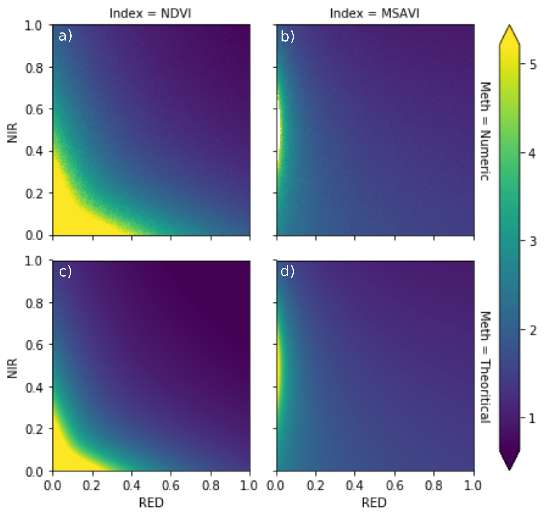
4.1. Selection of Vegetation Index

At a first approximation, the method is not addressed to a specific vegetation index and according to a general inference framework it assumes that the noise is normal and that the error is homogeneous (i.e., homoscedasticity). We can assume that the surface reflectance has an error which is approximately normal and that it is homogeneous for a not too high value, as it is possible to infer from the plots in [1]. However, the normality and homoscedasticity of errors is not guaranteed to be preserved after the index calculation. It is possible to estimate the expected uncertainties propagation for NDVI looking at the derivative of the formula [16]. We followed the same approach, a sum of square derivative in respect to both bands, using a symbolic derivative of the formula estimated with [17] for an MSAVI2 that has a very different Formula (7) but uses the same bands.
M S A V I 2 = ( 2 N I R + 1 ( 2 N I R + 1 ) 2 8 ( N I R R E D ) ) 2
To validate the theoretical approach, we also performed a simulation with 500 replicated, with the addition of a Gaussian white noise with standard deviation of 0.01, a rounded value of the mean standard deviations estimated in Table 1 for band 3 and 4 in [1]. Results are shown in Figure 4, where it is possible to notice that theoretical expectation and simulation match each other. Slightly higher dispersion in simulation is due to some negative values of reflectance that were not truncated. Looking at theoretical expectation only, it is possible to observe that MSAVI2 produces a much more homogeneous outcome with all values ranging between 1 and 2.5 times the error of input data, with the exception of the RED value of less than 0.1. On the contrary, NDVI, always ensuring the RED band a value greater than 0.1, ranges between 0.5 and 14 times the input error, thus making a difference in the expected standard error of 28 times across values of the same dataset. It is possible to observe a ratio output/input noise less than 1 in NDVI at a higher value of surface reflectance because it saturates at a higher level of vegetation cover [18], and thus representing another negative aspect of the index.
This observation leads us to use MSAVI2 for the rest of the analysis and to suggest the user of our approach to avoid normalized difference indices but seek more robust implementation of band normalization.

4.2. Simulation of Cloud Cover Experiment

To evaluate the performance of our approach on sparse and uneven distribution, we selected a subset of pixels in the Peneda Gerês dataset for which all observations were available. In this way, we selected 431 pixel series of 66 observations. We applied a 100 random cloud pattern found across the dataset to each of the pixel series, and estimated EFA for each year of observation, using both our method and the uncorrected data. Results are displayed in Figure 5, where the importance to correct the data to obtain credible EFA is clear: corrected data have lower spread and expectation is unbiased. The modelled data have some outliers farther away than raw data, but the five explored quantiles are generally less spread than raw data.

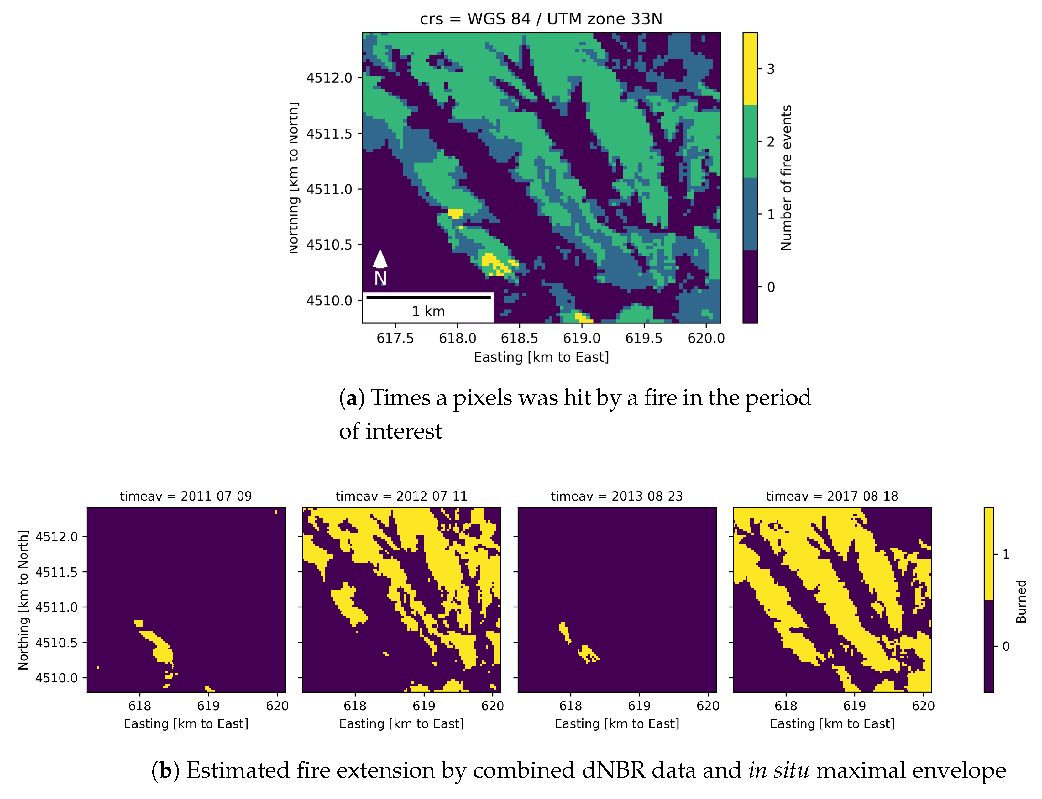
4.3. Testing over Forest Fires

To test the method’s sensitivity to change in seasonality, the performance was evaluated in case of events like forest fires, with a known date and a maximal extension. Two large fires and two smaller ones hit the region over the “Bosco Difesa Grande” (BDG) regional park from 2010 to 2017. The official maximal extension was taken from the national fire cadastre [19] and was compared with the results of a classical dNBR analysis (difference of the Normalized Burning Index in pre- and post-fire images [20]), using as threshold a decrease of 0.27 of the index, corresponding to “medium severity” or more (see also [21]). For the subsequent analysis, we considered the area that was hit by fire at the intersection of the two masks. In fact, dNBR was flagging few pixels outside the cadaster’s perimeter, probably due to some dry spots, while the cadaster is by construction an overestimated area (the convex hull includes all burned patches). For this evaluation, we also took into consideration the BFAST [7] program given that, differently from our approach, it explicitly models abrupt changes. The program requires an evenly sampled time series with a fixed number of observations per year with no missing data. We regularized the time series to 16 days, using a Savitzky–Golay filter, obtaining 182 scenes. We selected one year as the time between two breaking points, despite the advised value is four years [2]. The outputs of the two programs are not directly comparable, given that our approach produced statistics for each year, whereas BFAST produced statistics for each input date. We modified our approach to identify on the fitted data the day with maximum decrease rate (ratio between difference in fitted value and difference in time) per year and used this as an estimator of break to compare it with BFAST. In the comparison (Table 2, see also Appendix A), our approach (indicated as BM, also known as the Bayesian Model) shows much more favourable results both in terms of bias and in terms of average deviation. The particularly bad results for the 2017 fire of BFAST (expected value is 422.1 days before true value, with standard deviation of value of 271.1) are probably influenced by the scarce capacity to discriminate between two breaking points at about one year of distances to each other: the growth following the 2012 fire ended in 2016 (first breaking point), but a second fire hit the region in the following July (second breaking point), as shown in Figure 6.
The distances between the two events is approximately a year, and is therefore compliant with the setting that we imposed, but BFAST preferred for all pixels involved to fuse the two events. Summing the Trend and Seasonal components we built a BFAST expected value. From this, we built the same summary statistics as those of our approach. First, we built a linear model where the fire history, coded as four cipher binary variable, tried to predict the standard deviation across years estimated with our method and BFAST on each pixel. The results were very similar across our approach and BFAST, with both methods explaining 31.75% of variation. Second, for the 3-yearly EFA statistics, we built a similar linear model only for the four years when fire event had happened. For each of the four years we coded with 0 and 1 if the dNBR analysis had a decrease larger than 0.27, and added as predictor also the year of observation treating it a categorical variable, and 2011 (the first year of fire) was used as reference. Similar to the inter year standard deviation, the variance explained between the two approaches is very similar as reported in this instance (Table 3): BFAST greater than 2% in predicting the mean value, while our method results greater than 3.5% and 2.5% in predicting intra-year variation and day of maximum, respectively. Note that the negative coefficients for the unburned part in 2012–2017 for the yearly mean statistics are due to the very bad spring of 2012 and to the patch of old burned areas in the following years. Finally, we looked at the spatial and temporal local variation of the estimates. Both approaches observed the pixels through time without taking into account their respective spatial context, so in a good approach local variation should be much lower than overall scenes variation. As far as statistics are concerned, we chose median of standard deviation and we selected a 3 × 3 size kernel to define local neighbourhood. On the contrary, the standard deviation estimated from a temporal moving window of 3 × 3 size, should give values not too low compared to overall time variation. In fact, both approaches try to minimize a temporal variation, so the method that leaves more variation is more sensitive to changes. We reported the median value over the time series for the two approaches (Table 4). The result (Table 4) shows that our approach produces less local spatial variability than BFAST per day of maximum estimated (the ratio kernel std on total std is 0.207 versus 0.658 in BFAST), whereas for the other statistics our approach is only slightly better. Looking at the temporal local variation again, our method proves to be more effective in estimating the day of maximum with a higher local variation (0.643 versus 0.183). For the yearly variation (“std intra”), BFAST has a slightly higher value (0.708 over 0.560) which is not caused by a higher kernel variation, but by a lower overall variation.

4.4. Effect of Land Cover on Vegetation Phenology

To evaluate the quality of our prediction, we compared our results over the Murgia Alta National Park based on Landsat7-8 at 30 m with a land cover prediction inferred with an object based approach from four seasonal images of Worldview-2 (2 m resolution) taken in 19 April 2011, 5 October 2011, 22 January 2012 and 6 July 2012, respectively [22]. The landcover was inferred using the value of three indices (NDVI, WBI, Brightness) across the four images and comparing them with knowledge rule on the seasonality (natural phenology and agricultural practice) of the different land cover types. Finally, texture features were used to solve the difference between grassland and trees, and open and close land cover. For each 30 m tile, we calculated the proportion of the 16 land cover classes found within it, and used those values as predictor for the 3 EFA dimensions of 2012. Three linear models were built: one with EFA estimated from unmodified USGS data (Raw in Figure 7), one with data corrected with our approach (noW in Figure 7), and finally a weighted linear model using both our estimate EFA and the estimate error on the EFA estimate as weight (W in Figure 7). The weight was set as proportional to the inverse of the estimated standard deviation. In case our numerical estimate was zero, we set the weight as proportional to the inverse of one tenth of the smallest standard deviation recorded in the stack for that EFA dimension. The results show (Figure 7) that, regarding intra-year variation, the EFA dimension is best predicted by land cover mapping, closely followed by the mean values. Furthermore, in the consideration of the different estimates of EFA in terms of explained variance, the relation among dimensions remains the same and systematically in each dimension the best estimator results our approach, weighted by our estimates of error, whereas the least explained data are the EFA obtained by unmodified USGS data.

5. Conclusions

The aim of the present study is to show that the assumption of a regular time frame to collect summary statistics that allows using observations that are irregular and sparse, and yet to obtain robust and compelling statistics, as shown in our cloud cover experiment or in tracking multiple fire event test case. Furthermore, we took the stance to produce yearly statistics that are partially informed by long term observation. This is similar to what proposed in [23], but with the difference that we approached it in an explicit Bayesian framework and not within a rigid system of rules based on the number of observations available in each year. We are able to use the Bayesian framework using the conjugate prior and with the assumption that noise is normally distributed. This is quite a heavy assumption that holds on atmospherically corrected data, thanks to the multiple effect of overestimation and underestimation that the correction entails, and if no heteroscedasticity is added by the choice of the vegetation index as we show in the Section 4.1. The application of this method is limited, in a region with complex orography, by the need to correct data topographic errors such as shade or diffuse light. NDVI is said to be more robust to these effects, but to be used in this framework it is necessary to include explicit weight. We plan to do this upgrade in the next release of this software. Further development should go in the direction of producing statistics per object not per single pixel. This would allow to produce a more robust prediction. The software is distributed as open source on Github and will be available in the computation platform VLAB developed within the GeoEssential project. The portability is guaranteed by the availability of docker environment.

Author Contributions

Conceptualization, S.V., M.A. and D.A.-S.; methodology, S.V.; software, S.V.; validation, S.V. and M.A.; formal analysis, S.V.; investigation, M.A., C.T. and S.V.; data curation, C.T. and M.A.; writing—original draft preparation, S.V.; writing—review and editing, C.T., M.A. and D.A.-S. All authors have read and agreed to the published version of the manuscript.

Funding

We would like to acknowledge the support of H2020 Ecopotential project with Grant Agreement No. 641762 for the discussion and the set up of a first version of the algorithm not shown in this paper and Geoessential an ERA-PLANET project, an action from ERA-NET-Cofund Grant, with Grant Agreement No. 689443 for the actual development of the algorithm and the writing of the paper.

Acknowledgments

We would like to thank the ReCAS Computing Center of the University of Bari, and, particularly, Stefano Nicotri and Giacinto Donvito for the use of facilities; in particular their Jupiter online access to the virtual environment for computation. The manuscript was proofread by Lena Rettori. We would like to thanks the contribution of the two anonymous reviewers.

Conflicts of Interest

The authors declare no conflicts of interest. The founders had no role in the design of the study; in the collection, analyses, or interpretation of data; in the writing of the manuscript; or in the decision to publish the results.

Appendix A. Detailed Comparison of Fire Breaks

Figure A1. Comparison between estimation of maximum change near the first fire event. Histogram shows distribution of differences in day of the year between the actual fire event and the estimated one on the pixel that dNBR analysis identified as hit by this fire event. In the lower part, the two images show the spatial distribution in the two approaches. The projection used in the map is UTM zone 33N and extent and orientation is the same as Figure 2a in the main text.
Remotesensing 12 00083 g0a1
Figure A2. Same as Figure A1 for the second fire event.
Remotesensing 12 00083 g0a2
Figure A3. Same as Figure A1 for the third fire event.
Remotesensing 12 00083 g0a3
Figure A4. Same as Figure A1 for the forth fire event.
Remotesensing 12 00083 g0a4

References

  1. Ju, J.; Roy, D.P.; Vermote, E.; Masek, J.; Kovalskyy, V. Continental-scale validation of MODIS-based and LEDAPS Landsat ETM+ atmospheric correction methods. Remote Sens. Environ. 2012, 122, 175–184. [Google Scholar] [CrossRef] [Green Version]
  2. Forkel, M.; Carvalhais, N.; Verbesselt, J.; Mahecha, M.D.; Neigh, C.S.; Reichstein, M. Trend Change detection in NDVI time series: Effects of interannual variability and methodology. Remote Sens. 2013, 5, 2113–2144. [Google Scholar] [CrossRef] [Green Version]
  3. De Keersmaecker, W.; Lhermitte, S.; Honnay, O.; Farifteh, J.; Somers, B.; Coppin, P. How to measure ecosystem stability? An evaluation of the reliability of stability metrics based on remote sensing time series across the major global ecosystems. Glob. Chang. Biol. 2014, 20, 2149–2161. [Google Scholar] [CrossRef] [PubMed]
  4. Jianwen, L.; Yuke, Z. Comparison and application of NDVI time-series reconstruction methods at site scale on the Tibetan Plateau. Prog. Geogr. 2018, 37, 427–437. [Google Scholar] [CrossRef] [Green Version]
  5. Zhou, J.; Jia, L.; Menenti, M. Reconstruction of global MODIS NDVI time series: Performance of Harmonic ANalysis of Time Series (HANTS). Remote Sens. Environ. 2015, 163, 217–228. [Google Scholar] [CrossRef]
  6. Menenti, M.; Azzali, S.; Verhoef, W.; van Swol, R. Mapping agroecological zones and time lag in vegetation growth by means of fourier analysis of time series of NDVI images. Adv. Space Res. 1993, 13, 233–237. [Google Scholar] [CrossRef]
  7. Verbesselt, J.; Hyndman, R.; Zeileis, A.; Culvenor, D. Phenological change detection while accounting for abrupt and gradual trends in satellite image time series. Remote Sens. Environ. 2010, 114, 2970–2980. [Google Scholar] [CrossRef] [Green Version]
  8. Jönsson, P.; Eklundh, L. TIMESAT—A program for analyzing time-series of satellite sensor data. Comput. Geosci. 2004, 30, 833–845. [Google Scholar] [CrossRef] [Green Version]
  9. Nemani, R.R.; Keeling, C.D.; Hashimoto, H.; Jolly, W.M.; Piper, S.C.; Tucker, C.J.; Myneni, R.B.; Running, S.W. Climate-driven increases in global terrestrial net primary production from 1982 to 1999. Science 2003, 300, 1560–1563. [Google Scholar] [CrossRef] [PubMed] [Green Version]
  10. Alcaraz, D.; Paruelo, J.; Cabello, J. Identification of current ecosystem functional types in the Iberian Peninsula. Glob. Ecol. Biogeogr. 2006, 15, 200–212. [Google Scholar] [CrossRef]
  11. Regos, A.; Gagne, L.; Alcaraz-Segura, D.; Honrado, J.P.; Domínguez, J. Effects of species traits and environmental predictors on performance and transferability of ecological niche models. Sci. Rep. 2019, 9, 1–14. [Google Scholar] [CrossRef] [PubMed]
  12. Alcaraz-Segura, D.; Lomba, A.; Sousa-Silva, R.; Nieto-Lugilde, D.; Alves, P.; Georges, D.; Vicente, J.R.; Honrado, J.P. Potential of satellite-derived ecosystem functional attributes to anticipate species range shifts. Int. J. Appl. Earth Obs. Geoinf. 2017, 57, 86–92. [Google Scholar] [CrossRef]
  13. Arenas-Castro, S.; Regos, A.; Gonçalves, J.F.; Alcaraz-Segura, D.; Honrado, J. Remotely Sensed Variables of Ecosystem Functioning Support Robust Predictions of Abundance Patterns for Rare Species. Remote Sens. 2019, 11, 2086. [Google Scholar] [CrossRef] [Green Version]
  14. Walter, G.; Augustin, T. Bayesian linear regression—Different conjugate models and their (In)sensitivity to prior-data conflict. In Statistical Modelling and Regression Structures: Festschrift in Honour of Ludwig Fahrmeir; Physica-Verlag HD: Heidelberg, Germany, 2010; pp. 59–78. [Google Scholar] [CrossRef] [Green Version]
  15. Asher Bender. Bayesian Linear Model. Available online: https://github.com/asherbender/bayesian-linear-model (accessed on 6 November 2019).
  16. Borgogno-Mondino, E.; Lessio, A.; Gomarasca, M.A. A fast operative method for NDVI uncertainty estimation and its role in vegetation analysis. Eur.J. Remote Sens. 2016, 49, 137–156. [Google Scholar] [CrossRef]
  17. Wolfram. Wolframalpha. Available online: https://www.wolframalpha.com (accessed on 6 November 2019).
  18. Qi, J.; Chehbouni, A.; Huete, A.; Kerr, Y.; Sorooshian, S. A modified soil adjusted vegetation index. Remote Sens. Environ. 1994, 48, 119–126. [Google Scholar] [CrossRef]
  19. Catasto Incendi. Available online: http://www.simontagna.it/portalesim/catastoincendi.jsp (accessed on 6 November 2019).
  20. Keeley, J.E. Fire intensity, fire severity and burn severity: A brief review and suggested usage. Int. J. Wildland Fire 2009, 18, 116–126. [Google Scholar] [CrossRef]
  21. Heisig, J. Step by Step: Burn Severity mapping in Google Earth Engine. Available online: http://www.un-spider.org/advisory-support/recommended-practices/recommended-practice-burn-severity/burn-severity-earth-engine (accessed on 6 November 2019).
  22. Adamo, M.; Tarantino, C.; Lucas, R.M.; Tomaselli, V.; Sigismondi, A.; Mairota, P.; Blonda, P. Combined use of expert knowledge and earth observation data for the land cover mapping of an Italian grassland area: An EODHaM system application. In Proceedings of the 2015 IEEE International Geoscience and Remote Sensing Symposium (IGARSS), Milan, Italy, 16–31 July 2015; IEEE: Piscataway, NJ, USA; pp. 3065–3068. [Google Scholar] [CrossRef]
  23. Jönsson, P.; Cai, Z.; Melaas, E.; Friedl, M.A.; Eklundh, L. A method for robust estimation of vegetation seasonality from Landsat and Sentinel-2 time series data. Remote Sens. 2018, 10, 635. [Google Scholar] [CrossRef] [Green Version]
Figure 1. View of the three study sites over the backgrounds of Terrametrics TrueEarth 2019 images taken from google map services. In red the areas of interest, while in green the boundary of the protected areas. Peneda Gêres (a) is show in UTM29N projection, while Murgia Alta and, just south, Bosco Difesa Grande are shown in panel (b) using UTM33N projection. (c) The location of the area of interest are shown within European continent.
Remotesensing 12 00083 g001
Figure 2. Summary of the four fires that hit the “Bosco Difesa Grande” region as defined by dNBR analysis (difference of the Normalized Burning Index) and bounded by the fire cadastral delimitation. (a) The four fires are overlapped to observe the number of different fire event that hit each pixel area; (b) the view of each fire event. Very few experimented 3 fire events.
Remotesensing 12 00083 g002
Figure 3. Time of execution evaluation. The x-axis is relative at the value of the 3 different parameters. When one parameter is changed the others are fixed to 36 and 500 for yearly sample and replicates, respectively.
Remotesensing 12 00083 g003
Figure 4. Ratio between input and output noise for different values of surface reflectance NIR and RED. In panels (a,c) data are relative to NDVI, while the others to MSAVI2. In panels (a,b) data are obtained from numerical simulation with 500 replicates per pair of surface reflectance values, whereas (c,d) resulted from the derivative approach.
Remotesensing 12 00083 g004
Figure 5. Distribution of difference between 423 EFA values across 6 years (2005–2010) in the Peneda Gerês data set, estimated with a full set of observations and applying on them 100 different cloud patterns. Estimates with modelled and raw data are respectively blue and orange. In subfigure (ac) are shown yearly mean and stardard deviation, day of the year of maximum and number of observation per year, respectively.
Remotesensing 12 00083 g005
Figure 6. Summary of the Breaks For Additive Season and Trend (BFAST) reconstruction over the pixel that experienced 2012 and 2017 fire based on dNBR analysis. In green the observation after Savitzky–Golay filter, in dark red the median of the BFAST expectation, in cyan the median of pre-2012 expectation. Vertical dark red line represent BFAST estimation of breaking point, whereas bright red is the actual fire event. Take note that median estimation and 2.5 and 97.5 quantile of breaking point estimation overlap in the figure.
Remotesensing 12 00083 g006
Figure 7. Variance explained by land cover frequency over the summary statistics.
Remotesensing 12 00083 g007
Table 1. Dataset used in this work.
Name LocalityScenes n ° X Cells n ° Y CellsYears Span
Peneda Gerês66252124582005–2010
Murgia Alta53811224882000–2018
Bosco Difesa Grande19287962010–2017
Table 2. Bias and average deviation in days of the two methods (our proposed method, BM, and the reference, BFAST) compared to the true date of fire over the pixel characterized by dNBR smaller than −0.27, estimated using pairs of Landsat image before and after the known fire date. Negative value of bias indicates the estimated date prior true date. In each case the nearest break was used to estimate the statistics.
BiasStd
Method Fire EventBMBFASTBMBFAST
27 June 201133.3118.251.2196.1
30 June 201221.4−29.947.6110.6
15 August 2013−17.715.762.5245.6
12 August 2017−3.1−422.151.4271.1
Table 3. Results from 4 linear models for yearly mean and yearly standard deviation estimated with our approach (BM) and BFAST that use year of observations and fire events (estimated from dNBR) as predictors. We report the coefficient and the variance explained, adjusted by number of parameters (Rsq adj).
mean_meanstdintra_meanmaxpos_mean
BMBFASTBMBFASTBMBFAST
Intercept (2011:nofire)0.3300.3220.0900.080144.206145.140
2012:nofire−0.038−0.053−0.007−0.006−4.431−13.457
2013:nofire−0.053−0.041−0.0050.004−8.7223.898
2017:nofire−0.0110.0060.0060.0075.722−8.013
fire−0.076−0.069−0.003−0.000−26.258−29.640
2012:fire0.0230.0290.0040.01113.92434.929
2013:fire0.0710.0770.012−0.0084.70335.068
2017:fire0.0270.0130.018−0.00619.34826.071
Rsq_adj0.1620.1820.0480.0130.0650.041
Table 4. Spatial and time local variation of estimates across methods (our proposed ones, BM, and BFAST), using standard deviation as metric. A kernel of 9 pixels and a moving window of 3 were used respectively for space and time domains. For each summary statistic, the mean kernel, the overall and the ratio of the two values are reported.
SpaceTime
BFASTBMBFASTBM
maxposkernSD18.2895.9451.2474.490
TotSD27.78728.7486.8196.986
Rate0.6580.2070.1830.643
meankernSD0.0210.0210.0270.022
TotSD0.0670.0660.0360.029
Rate0.3190.3210.7470.766
std intrakernSD0.0140.0140.0070.007
TotSD0.0360.0380.0090.013
Rate0.3860.3780.7080.560
std interkernSD0.0060.006--
TotSD0.0360.038--
Rate0.1530.146--

