Geostationary Ocean Color Imager (GOCI) Marine Fog Detection in Combination with Himawari-8 Based on the Decision Tree

Abstract

Geostationary Ocean Color Imager (GOCI) observations are applied to marine fog (MF) detection in combination with Himawari-8 data based on the decision tree (DT) approach. Training and validation of the DT algorithm were conducted using match-ups between satellite observations and in situ visibility data for three Korean islands. Training using different sets of two satellite variables for fog and nonfog in 2016 finally results in an optimal algorithm that primarily uses the GOCI 412-nm Rayleigh-corrected reflectance (R_rc) and its spatial variability index. The algorithm suitably reflects the optical properties of fog by adopting lower R_rc and spatial variability levels, which results in a clear distinction from clouds. Then, cloud removal and fog edge detection in combination with Himawari-8 data enhance the performance of the algorithm, increasing the hit rate (HR) of 0.66 to 1.00 and slightly decreasing the false alarm rate (FAR) of 0.33 to 0.31 for the cloudless samples among the 2017 validation cases. Further evaluation of Cloud-Aerosol Lidar and Infrared Pathfinder Satellite Observation data reveals the reliability of the GOCI MF algorithm under optically complex atmospheric conditions for classifying marine fog. Currently, the high-resolution (500 m) GOCI MF product is provided to decision-makers in governments and the public sector, which is beneficial to marine traffic management.

1. Introduction

Fog is a type of cloud whose base is at the Earth’s surface. Small water droplets in the atmosphere near the surface reduce visibility and significantly affect human activities. According to international definitions, fog occurs when the visibility is less than 1 km [1]. Marine fog (MF) is one of the most dangerous weather hazards that threaten coastal and marine human activities. It impedes ship navigation due to the low visibility, and affects inland traffic systems by intruding onto land. Approximately 32% of all ship traffic accidents at sea occur in the presence of dense MF [2]. MF also severely limits visibility in aviation. Advection fog often affects airports along coastlines across the U.S., Europe, Asia, etc. Both wide-area and focused surveillance of MF are necessary for timely warnings to the public and decision-makers to lessen the damage due to marine and air traffic accidents.

Whereas land fog has a relatively dense observational network via visibility meters at most meteorological stations, MF observations are distinctly sparse. Ship observations focus primarily on ocean physical properties, such as sea surface temperature, temperature profile, salinity, etc. Due to the absence of regular visibility observations over the ocean, the remote sensing of MF is the best method. Often, coastal points (ports, bridges, etc.) along complex coastlines require MF monitoring. In South Korea, the length of the coastline is approximately 14,963 km, and it accounts for up to 37% of the circumference of the Earth [3]. In this case, information with a high spatial resolution is necessary to detect the regional distribution of MF in coastal areas. The near-real-time detection of MF is also important, because it can form, advect and dissipate in several hours. Therefore, it is appropriate to use geostationary satellites rather than polar-orbiting satellites, whose data are generally available only once or twice a day in the low/mid-latitudes. In this study, the Geostationary Ocean Color Imager (GOCI) onboard the Communication, Ocean and Meteorological Satellite (COMS) with a resolution of 500 m is applied to local and synoptic-scale monitoring of MF over the Yellow Sea, Korean Strait and the East Sea (Japan Sea).

For more than three decades, satellite-based fog detection methodologies have been developed [4,5,6,7,8,9]. Previous studies have utilized the dual channel difference (DCD) between shortwave infrared (IR) (SWIR) and longwave IR (LIR) or visible (VIS) channels. Since IR window channels (e.g., 10.8 μm) can provide cloud height information through the cloud top temperature, it can classify higher cloud (deep cumulonimbus or high cirrus clouds) from fog just above the underlying surface [4]. Eyre [5] first suggested using the difference in brightness temperature (BT) between SWIR (3.9 μm) and LIR (10.8 μm) channels called the DCD. The emissivity in the SWIR range is lower than that in the LIR range for clouds with small water droplets (i.e., fog or stratus clouds), while both emissivities are roughly the same for larger droplets [6]. Ellrod [7] tried to detect fog at night based on the DCD method with the Geostationary Operational Environmental Satellite. The results showed that the DCD method is effective for fog detection across a wide range of terrain and temperature regimes if fog is not obscured by any clouds above. However, the DCD method has limitations in detecting shallow fog, especially in winter, because an excessively small DCD value falls within the range of instrument noise. In addition, the use of the 3.9-μm channel for daytime fog detection remains difficult in setting a stable threshold due to the mixed effect of solar and Earth radiation [8].

On the other hand, VIS channels are suitable for fog detection in the daytime. In the daytime, fog areas appear bright in the visible image since they strongly reflect solar radiation [5]. Anthis and Cracknell [9] used both IR and VIS channels for fog detection over lowland Thessalia. The IR channel data from the Advanced Very-High-Resolution Radiometer (AVHRR) and VIS channel data from METEOSAT are used to detect fog at night and to predict the dissipation of fog in the daytime, respectively.

Several fog detection studies have been conducted around the Korean Peninsula by using AVHRR [10], MTSAT-1R [11] and COMS/MI [12]. Additionally, there have been several studies focused on MF near the Korean Peninsula [13,14,15]. Heo et al. [13] attempted to distinguish MF from low stratus clouds using the homogeneity between the IR channel and DCD from the Moderate Resolution Imaging Spectroradiometer (MODIS). Gao et al. [14] also used the DCD method with MTSAT-1R data for nighttime MF/stratus cloud detection over the Yellow Sea. Recently, Yuan et al. [15] developed an algorithm using the GOCI VIS reflectance by setting spectral thresholds for MF classification. They reported that their algorithm is generally accurate over the Yellow Sea. However, due to the lack of longwave IR bands in the GOCI, it is hypothesized that only using visible bands may have fundamental limitations in classifying fog from cloud pixels.

In this study, we applied GOCI VIS data together with IR-observable meteorological satellite data for the detection of MF over East Asian seas, including the Yellow Sea, the Korea Strait and the East Sea. A new MF detection algorithm was developed based on the decision tree (DT) approach. The DT method has a significant potential for developing remote sensing algorithms [16]. Compared to other machine learning techniques, the DT method has clear rules and relationships among the variables [17,18].

One of the primary focuses of this study is whether the combined use of GOCI and Himawari-8 data improves the performance of MF detection. Then, another major consideration is to develop a new method to combine information from two satellites for fog detection.

Section 2 describes the data used, GOCI and Himawari-8 satellite data, visibility data from weather stations, Cloud-Aerosol Lidar and Infrared Pathfinder Satellite Observation (CALIPSO) data, and provides details on the construction of satellite–weather station match-up data for the training and validation of the proposed algorithm. Section 3 describes the methodologies of the DT approach, satellite input indices and training and validation of the GOCI MF algorithm. Section 4 includes the results of the DT approach, postprocessing via combining with Himawari-8 and validation. An additional validation of the GOCI MF algorithm based on the vertical cloud structure observation by CALIPSO data is provided in Section 5. A summary and the conclusions are presented in Section 6.

2. Data

2.1. COMS/GOCI

The GOCI is one of the payloads of the first Korean geostationary satellite, COMS, which was launched in June 2010. The GOCI has six narrow-width visible (412, 443, 490, 555, 660 and 680 nm) and near-infrared (745 and 865 nm) bands to observe short-term and long-term changes in the coastal ocean environment for marine science research and application purposes [19,20,21]. The spatial resolution of the GOCI is approximately 500 m, and the range of the target area is approximately 2500 km × 2500 km around the Korean Peninsula (e.g., Figure 1). The GOCI provides hourly images eight times (from 00 UTC to 07 UTC) a day. To develop an objective algorithm to determine MF and nonmarine fog regions from GOCI images, this study utilizes the GOCI Rayleigh-corrected reflectance (R_rc), in which the atmospheric scattering effect (including cloud particles and aerosols) remains except for atmospheric molecular scattering. R_rc can be computed from the top-of-atmosphere (TOA) radiance (L_TOA) observed at the satellite level as follows:

$${\rho }_{TOA}\left(\lambda \right)=\frac{\pi L_{TOA}\left(\lambda \right)}{F_0\left(\lambda \right)\cos {\theta }_s},$$

(1)

$$R_{rc}\left(\lambda \right)={\rho }_{TOA}\left(\lambda \right)-{\rho }_r\left(\lambda \right),$$

(2)

where ρ_TOA is the TOA reflectance, F₀ is the extra-terrestrial solar irradiance, θ_s is the solar–zenith angle. The term ρ_r is the Rayleigh multiple-scattering reflectance in the absence of aerosols that can be accurately calculated from given solar-sensor geometry, air-pressure and wind speed at sea surface [22,23,24,25,26]. Based on optical analysis of the various bands, R_rc at 412 nm will be used for our algorithm (Section 3.2).

2.2. Himawari-8/Advanced Himawari Imager (AHI)

Himawari-8 is the geostationary weather satellite operated by the Japan Meteorological Agency since 2015 [27]. A payload called the AHI is a multispectral imager that has 16 channels (0.47, 0.51, 0.64, 0.86, 1.6, 2.3, 3.9, 6.2, 6.9, 7.3, 8.6, 9.6, 10.4, 11.2, 12.4 and 13.3 µm). The AHI captures visible and infrared images of the Asia-Pacific region and provides full-disk observations every 10 minutes. In this study, we tested various Himawari-8 products, such as cloud top height (CLTH), infrared (10.4 µm) BT and sea surface temperature data, together with the GOCI R_rc. Only the CLTH information was used for the proposed algorithm (Section 3.3). Since the spatial resolution of the Himawari-8 CLTH is 5 km, bilinear interpolation was performed to match Himawari-8 pixel values to GOCI pixels with a resolution of 500 m.

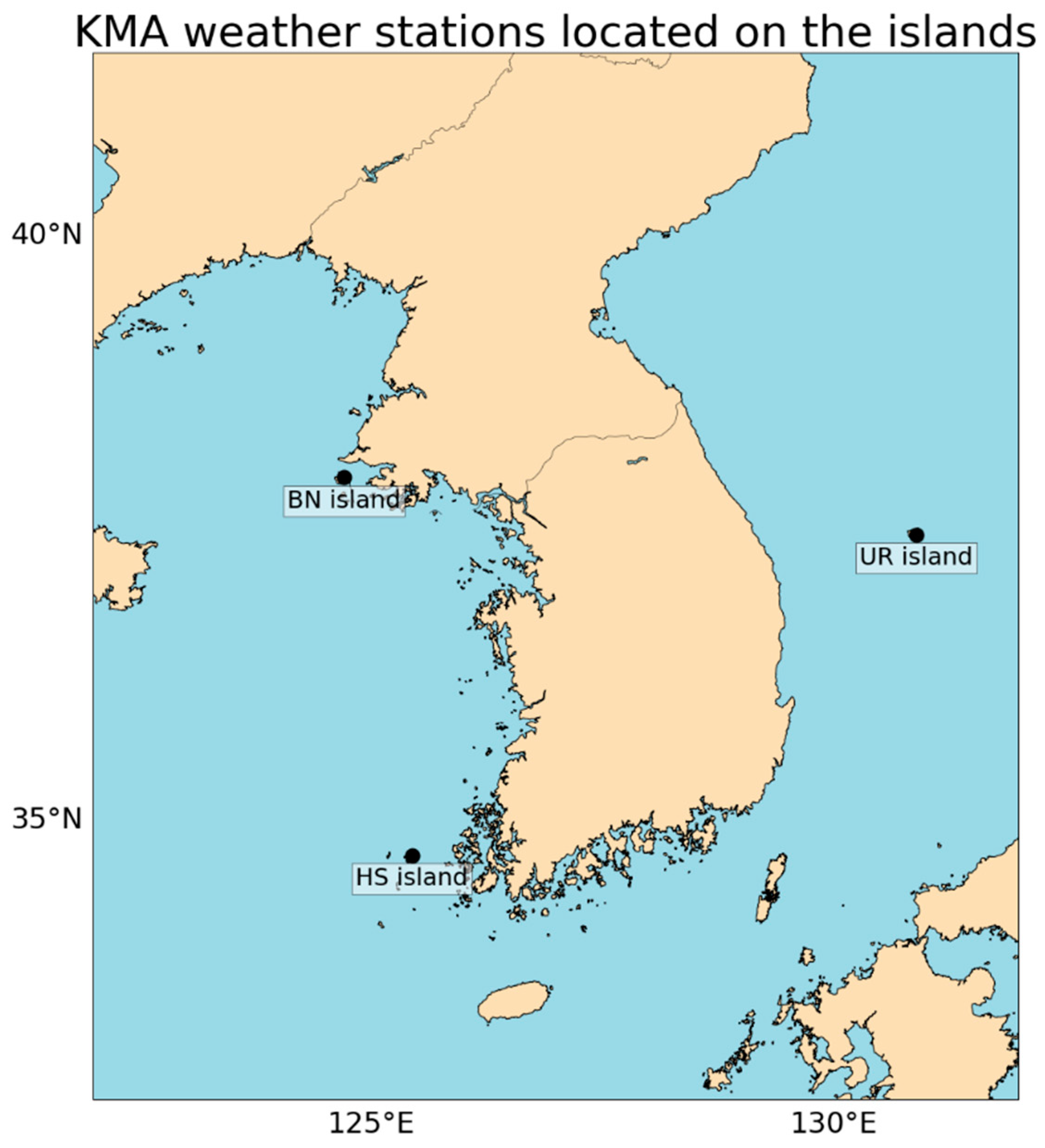
2.3. Automated Synoptic Observing System (ASOS) of the Korean Meteorological Administration (KMA)

This study uses visibility observations at the synoptic weather stations operated by the KMA. To confirm MF and nonmarine fog regions, we use the visibility observations at three islands: Baengnyeong (BN), Heuksan (HS) and Ulreung (UR), as shown in Figure 2. The visibility in meters is the maximum distance that a predefined object can be clearly discerned on the surface. If the visibility differs depending on the direction, the minimum value is selected. In ASOS, the visibility is measured with optical visibility sensors produced by the Belfort Instrument (6550), Vaisala (PWD-22) or Biral (VPF-730) companies. The optical visibility sensor transmits and receives a laser beam to calculate the visibility by using the principle that the degrees of light scattering and absorption are attenuated by particles in the air [28,29,30].

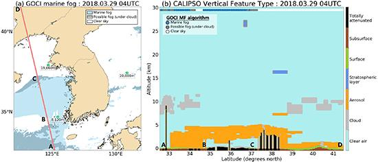
2.4. The Cloud-Aerosol Lidar and Infrared Pathfinder Satellite Observation (CALIPSO)

The Cloud-Aerosol Lidar with Orthogonal Polarization (CALIOP) instrument onboard the CALIPSO satellite was used for algorithm validation. The CALIOP with 532 nm and 1064 nm bands has been the primary instrument for performing global profiling of the aerosols and clouds in the troposphere and lower stratosphere since 2006 [31]. It combines an active lidar instrument with passive infrared and visible imagers to investigate three-dimensional structures of cloud particles and aerosols (https://www-calipso.larc.nasa.gov/). CALIOP footprints are produced every 335 m with a diameter of ~70 m. We use CALIOP level 2 Vertical Feature Mask (VFM) data. The VFM provides information on the locations and types of clouds and aerosols over wide ocean areas where in situ visibility observations are unavailable. The vertical and horizontal resolutions vary depending upon the height. The vertical (horizontal) resolutions are 30 (333), 60 (1000) and 180 (1667) m at heights of 0.5–8.2, 8.2–20.2, and 20.2–30.1 km, respectively.

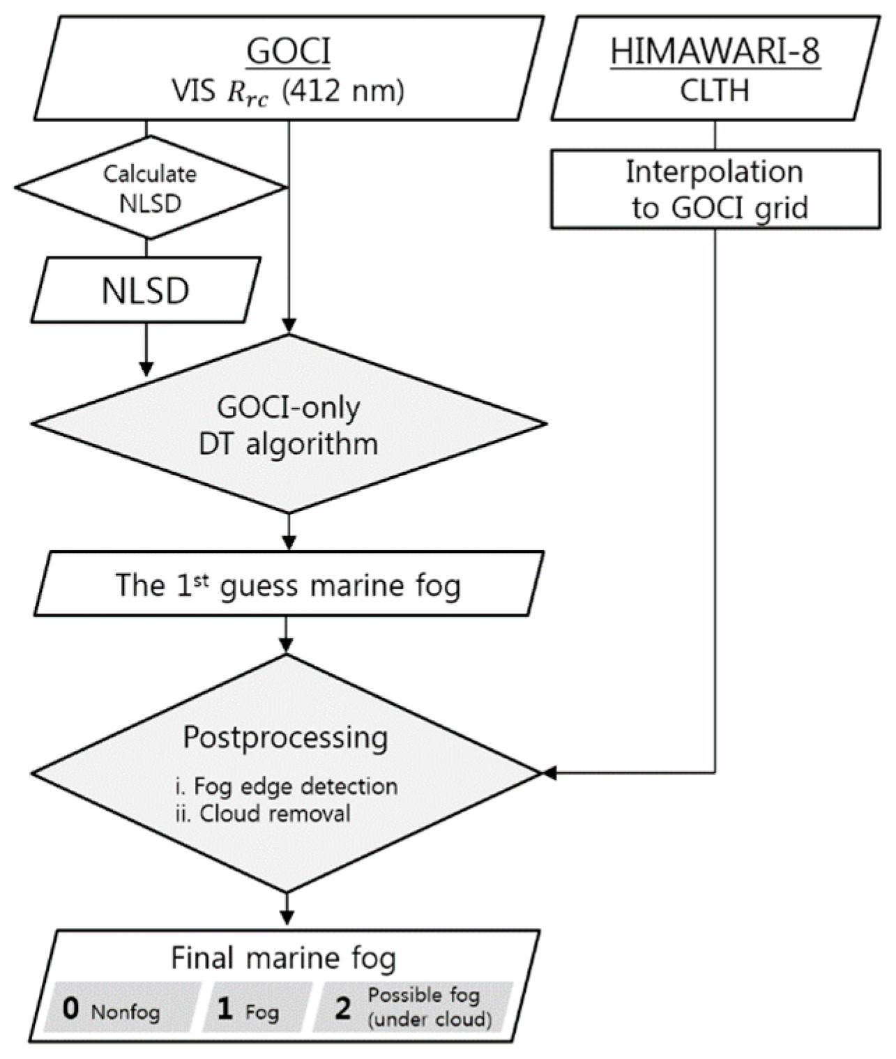
3. Methodology and Model Development Procedure

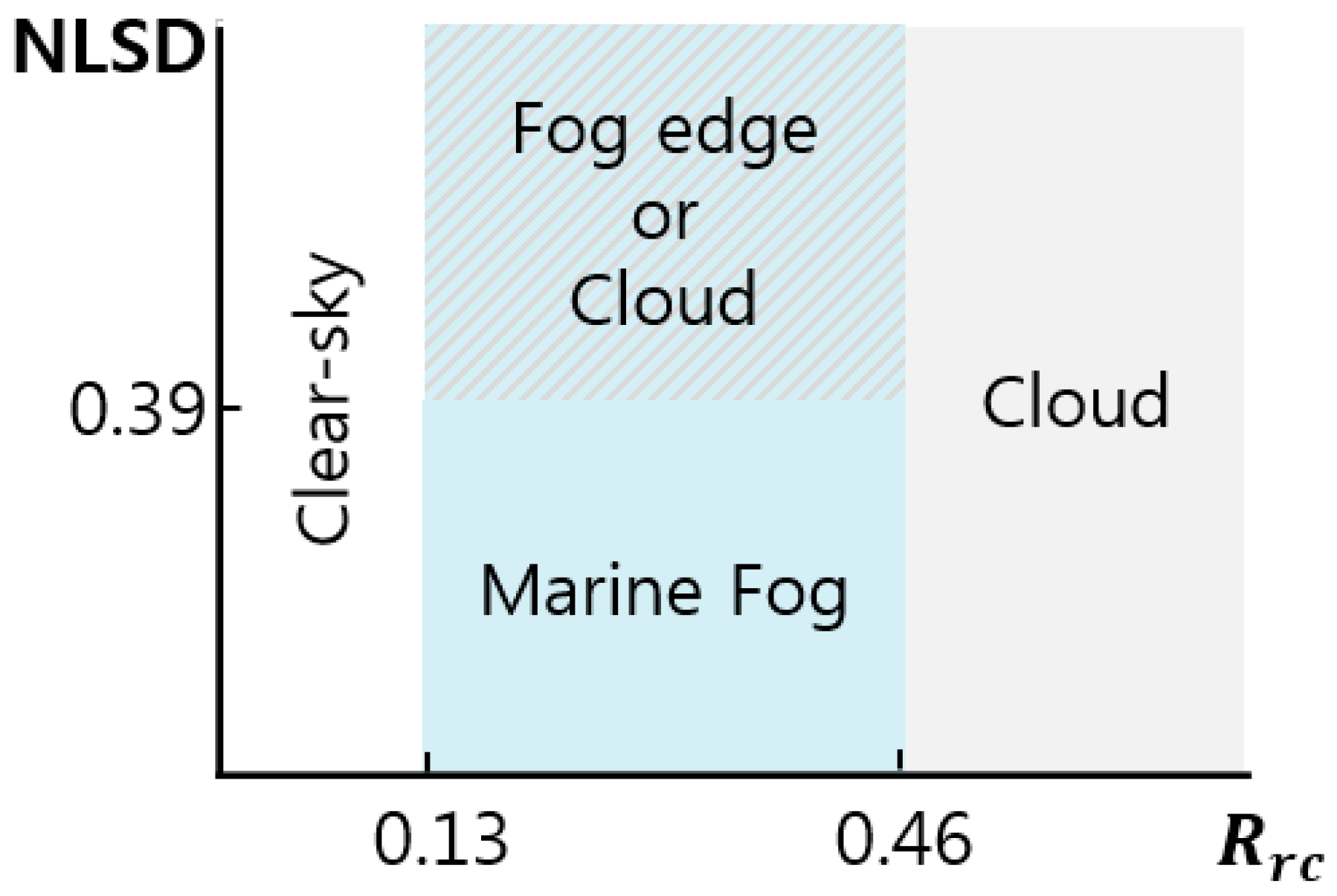
3.1. Decision Tree (DT)

The MF detection algorithm in this study was developed using the DT method, a type of machine learning algorithm [32]. The DT has been applied to the development of remote sensing algorithms [16,17,18,33,34]. The application of the DT allows a physical interpretation of the logical relationship between input variables and the final remote sensing algorithm product, since it visualizes the classification rules in a treelike structure [17]. In this study, the ‘rpart’ package of R, which is one of the DT packages, was used. The ‘rpart’ package is based on the classification and regression tree (CART) [35] algorithm. The CART is a binary DT that is constructed by a splitting a node into two child nodes repeatedly using the Gini index. The CART approach makes the tree sufficiently large until there are no new divisions to improve performance. Next, the predictive ability of the final tree is enhanced through the pruning process.

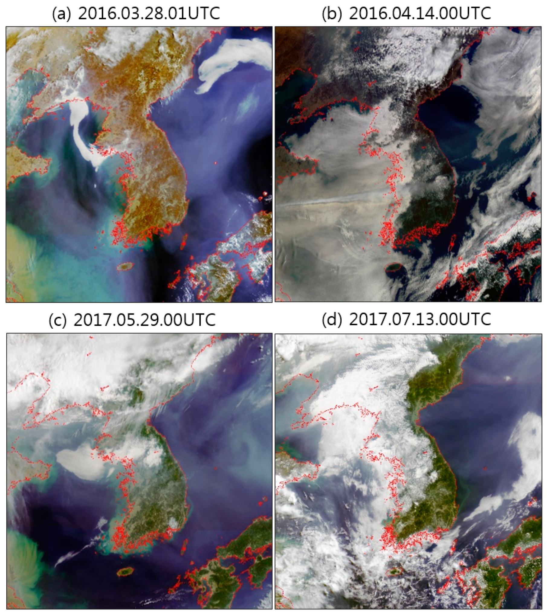
3.2. Satellite-Weather Station Match-Up Data for Training and Validation

The development of machine learning-based remote sensing algorithms requires the construction of match-up data between satellite and in situ observations of MF and nonmarine fog samples. The first procedure is to collect GOCI images based on visual analysis by a satellite analysis expert. For the MF samples, we selected approximately 30 fog candidate GOCI images, and four examples are shown in Figure 1. In the RGB images of 28 March 2016 (Figure 1a), MF with a distinct white color and smooth texture occurs along the northern part of the Yellow Sea and the East Sea (Sea of Japan) without notable clouds above. On 16 April 2016 (Figure 1b), MF spreads more widely across the Yellow Sea and the East Sea. However, a narrow band of higher clouds passes over the fog across the Yellow Sea. A heart-shaped fog region is located to the east of the Shandong Peninsula on 29 May 2017 (Figure 1c). On 13 July 2017 (Figure 1d), fog across the Yellow Sea is mixed with clouds, revealing a rough texture to the south.

Using many fog candidate GOCI images, the second step is to confirm satellite MF pixels using the KMA visibility data from the islands of BN, HS and UR (Figure 2). If the visibility is less than 1 km, pixels within a 2 km radius of the station were confirmed as MF samples. Because approximately 50 GOCI pixels are included in the 2-km radius circle, a radius of less than 2 km results in a sample size that is too small for training /validation. In this step, through the homogeneous test, we excluded fog boundary areas, i.e., cases in which fog and nonfog regions coexist.

Similarly, the nonmarine fog samples are obtained. After selecting cloud and cloud-free cases through visual interpretation of GOCI RGB images, we chose cases where the visibility at three specific weather stations was greater than 1 km. By applying the Himawari-8 CLTH, we collected clear-sky, low-level cloud (CLTH < 3 km), mid-level cloud (3 km < CLTH ≤ 7 km) and high-level cloud (CLTH ≥ 7 km) samples. Lastly, the GOCI pixels within a 2-km radius with a visibility > 1 km at the KMA stations were defined as nonmarine fog samples.

Table 1. List of marine fog cases used as training and validation data. The station represents the location where the samples were obtained. These cases were selected by the match-up process between satellite and in situ data (the station number is the KMA weather station number) or subjective RGB image analysis (the station longitude and latitude are listed). Station numbers 102, 169 and 115 are the islands of Baengnyeong, Heuksan and Ulreung, respectively.

Training
Year	Month	Day	Hour (UTC)	Station number or location
2016	3	28	1	102
	4	8	1	102/169/124.8°E, 39.28°N
	4	8	5	124.8°E, 39.28°N
	4	14	0	102/169
	4	14	1	102/169
	4	14	2	102/169
	4	14	3	169
	4	14	4	169
	4	14	7	102
	4	22	0	102/169
	4	22	1	102
	4	22	2	102
	4	22	3	102
	7	25	1	102
	7	25	2	102
	7	25	3	102
Validation
Year	Month	Day	Hour (UTC)	Station number or location
2017	3	5	5	102
	4	6	0	102
	4	6	1	102
	4	6	7	115
	4	15	0	102
	4	25	0	102
	5	25	0	115
	5	29	0	102
	5	29	1	102
	5	31	6	169
	5	31	8	169
	7	11	0	102
	7	13	0	102
	7	13	0	169
	7	14	0	102

shows the dates and times of the confirmed MF cases that will be used for training and validation.

Note that the samples were basically obtained through the abovementioned match-up process with the KMA data. However, our earlier DT training results showed that the algorithm was not effective in detecting thin fog (results not shown in this article). The exclusion of fog boundary areas from the MF samples may have resulted in the inclusion of thicker fog but not thinner fog. It is necessary to include fog systems with a range of thicknesses to improve the versatility of the developed algorithm for a range of applications. Accordingly, additional thin fog samples were added based on visual RGB image analysis results, which are included with longitude and latitude information in Table 1.

Table 2. The number of marine fog and nonmarine fog samples obtained through the match-up process between satellite and in situ data. Each number represents the number of pixels corresponding to marine fog or nonmarine fog. The 2016 and 2017 data were used as training and validation data, respectively, for the marine fog detection algorithm.

Marine fog Classification	Data	Training	Validation
1	Marine fog (2016)	4868
	Marine fog (2017)		1281
0	Nonmarine fog (2016)	7875
	Nonmarine fog (2017)		1592
Total number		12,743	2873

summarizes the numbers of final MF and nonfog samples, and the 2016 and 2017 samples were used as training and validation data, respectively. A total of 12,743 (2873) pixels, 4868 (1281) fog and 7875 (1592) nonfog pixels, were used for training (validation). In this study, validation was conducted in two different ways using the in situ visibility and the CALIPSO data. First, basic validation was conducted using the 2017 sample dataset, as summarized in Table 2, and the hit rate (HR), false alarm rate (FAR), miss rate (MR) and negative hit rate (NHR) of the developed algorithm are presented. Here, the HR (NHR) is the ratio of correctly detected MF (nonmarine fog) to the actual MF (nonmarine fog). FAR (MR) is the ratio of incorrectly detected MF (nonmarine fog) to the actual nonmarine fog (MF). In addition to using the validation samples (2017) in Table 2, further near-real-time evaluation is also performed using in situ visibility observations and CALIPSO data (Section 5.2)

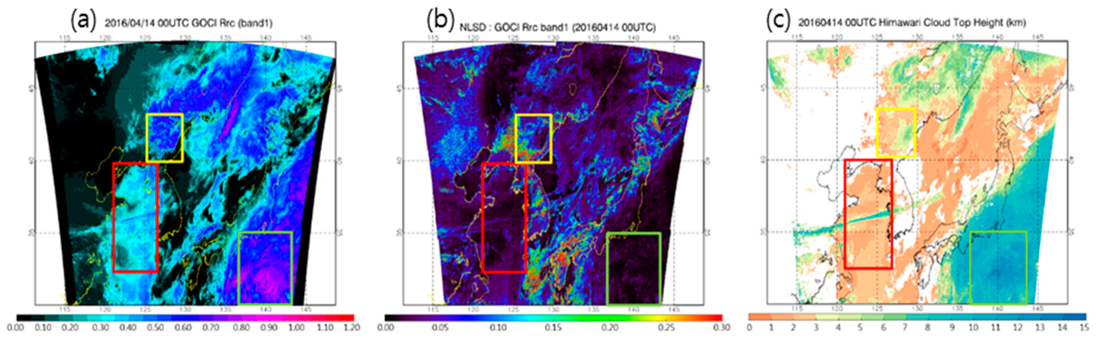
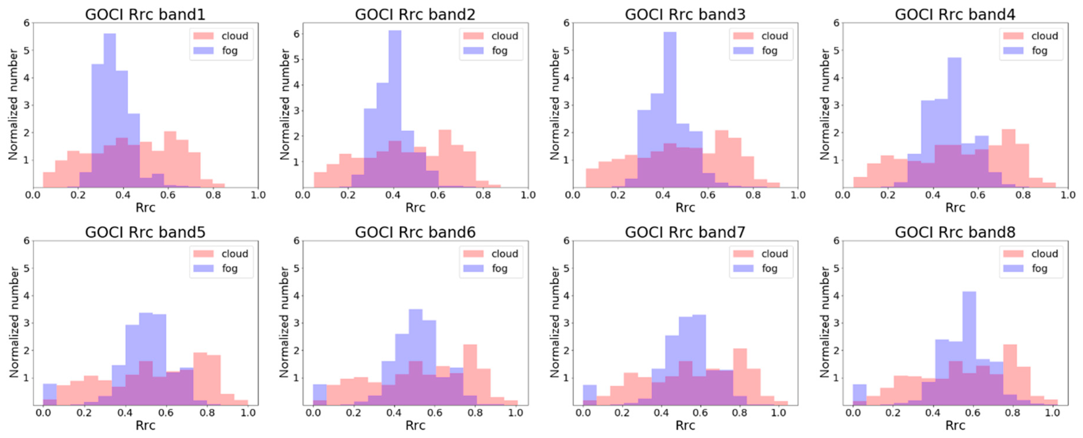
3.3. Satellite Input Variables for the MF Algorithm

Using the GOCI and Himawari-8 data, we investigate satellite variables and indices to characterize the optical and textural properties of MF for their classification from other cloudy or clear pixels. As mentioned in Section 1, the BT of the IR channel, DCD and reflectance of the visible channel are representative variables for fog detection, and they were all considered candidate input variables.

The GOCI band 1 Rrc is selected as the primary input to classify fog from clouds. Generally, as shown in Figure 3a, the Rrc values for fog are higher than those for clear sky, but lower than those for high-level clouds. As shown in Figure 4, we investigate the distribution of Rrc of all GOCI bands for fog versus nonmarine fog (mid- and high-level clouds). For all bands, the Rrc for the fog pixels tends to have a narrow distribution, and their peak increases from 0.3 to 0.6 as the band number increases from 1 to 8. Clouds, on the other hand, have a much broader distribution due to their various thickness features. The Rrc median values for each GOCI band are listed in

Table 3. Median of $R_{rc}$ for marine fog and cloud samples and difference between the samples.

GOCI Band	Median of Rrc		Difference
	Fog	Cloud
1	0.36	0.44	0.08
2	0.39	0.46	0.07
3	0.43	0.49	0.06
4	0.47	0.52	0.05
5	0.51	0.56	0.05
6	0.52	0.56	0.04
7	0.55	0.58	0.03
8	0.56	0.58	0.02

. The difference between fog (0.36) and clouds (0.44) is the largest for band 1 among all bands, which motivated us to use the Rrc of band 1.

However, it is reasonable that due to thin or low-level clouds, only using R_rc is not enough to properly distinguish MF from the various types of clouds. To improve the cloud removal procedure, additional inputs for the algorithm include the spatial variability index of R_rc and the Himawari-8 CLTH information. The CLTH is very useful for removing clouds that are higher than fog. As shown in Figure 3c, high clouds (green box) can be easily distinguished from fog (red box) using the CLTH.

We first considered the Himawari-8 IR BT data as input data for our MF algorithm due to their relationship with cloud height information by measuring the cloud top temperature. However, the IR BT has a disadvantage because it is highly sensitive to changes in the surface environment, such as the sea surface temperature. As shown in Figure 5, the IR BT for MF cases has much larger seasonal variations than the GOCI R_rc and NLSD, which implies difficulties in setting fixed thresholds for the IR BT in classifying fog without proper correction of the sea surface temperature. For this reason, we use the GOCI visible and Himawari-8 CLTH data due to their lower sensitivity to environmental changes.

Using the CLTH remains insufficient for MF classification from low clouds (yellow box, Figure 3c) with similar cloud top heights as those of fog (red box, Figure 3c). Therefore, a pattern index of the GOCI R_rc is defined to improve the distinction between MF and low clouds. Homogeneity is useful information, because fog and clouds have different roughness patterns in satellite images. The top surface of MF is relatively flat under stable atmospheric conditions, whereas that of clouds is uneven due to alternating upward and downward motions [36].

As a spatial pattern index, the normalized local standard deviation (NLSD) of R_rc is calculated with surrounding pixels (9 × 9) using the equation below:

$$\mathrm{NLSD}=\frac{Local standard deviation}{Local mean },$$

(3)

Figure 3b shows that the NLSD is an effective index for separating MF from low clouds. The NLSD value for MF (red box) is lower than that for low clouds (yellow box). In this section, the input variables for the MF detection algorithm are determined as the GOCI R_rc (band 1), NLSD, and Himawari-8 CLTH.

4. Results

The developed MF detection algorithm (Figure 6) is designed to conduct two steps: (i) GOCI MF detection based on the DT approach and (ii) postprocessing for improving cloud removal and fog edge detection using Himawari-8 data, which will be explained in the following two subsections.

4.1. GOCI MF Detection Algorithm: DT-Trained Results

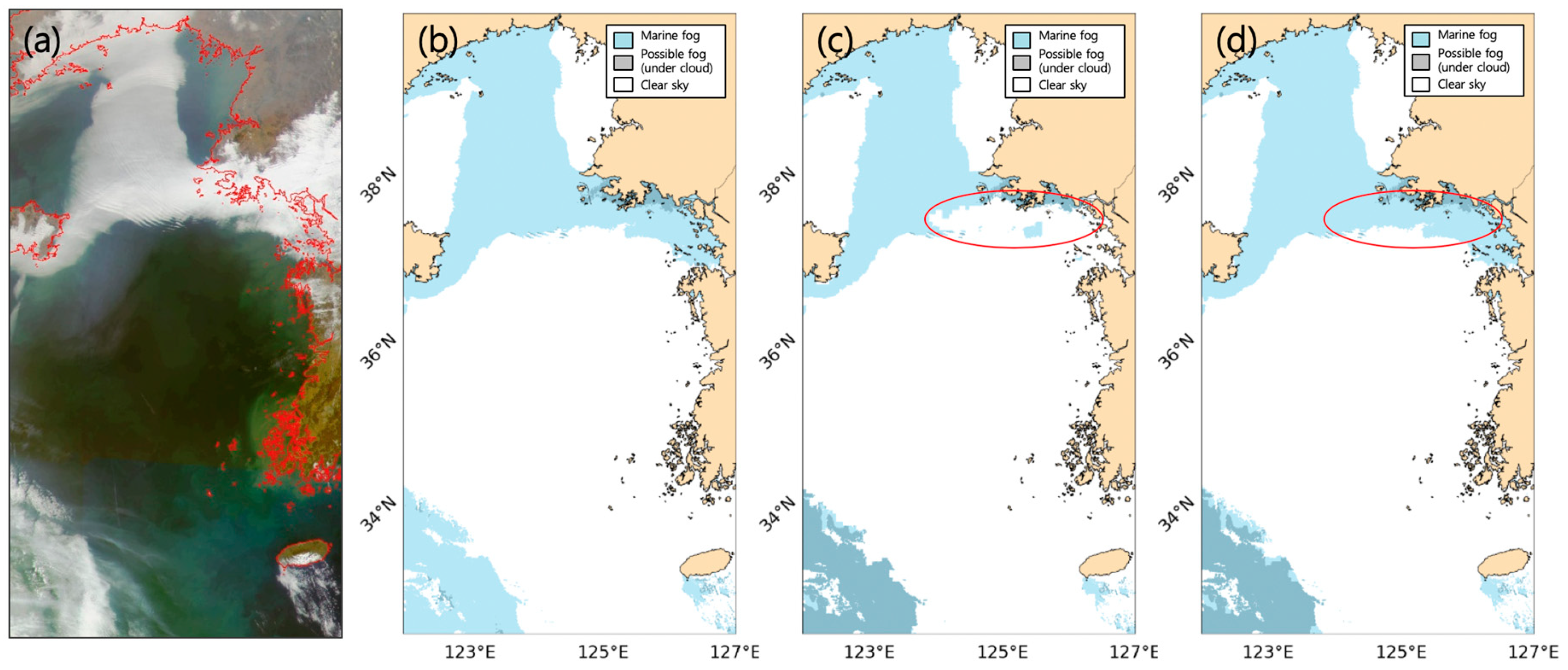
The GOCI 412-nm R_rc and NLSD indices were used as the primary input variables for the DT algorithm to classify MF (Figure 6). The structure of the trained algorithm through the DT algorithm is presented in Figure 7. Pixels with R_rc values lower than 0.13 are classified as clear-sky pixels and have a very low R_rc value. In contrast, pixels with R_rc values ≥ 0.46 are identified as clouds, due to their large optical thickness. On the other hand, medium-range R_rc (0.13 < R_rc ≤ 0.46) pixels may include fog and thin clouds. Among these pixels, only pixels with a lower R_rc spatial variability (NLSD < 0.39) are classified as MF, which indicates a smoother top surface. As a result of the DT, the first guess of MF pixels is designated as the interim product. The rules of the DT appropriately follow the general understanding of optical properties and fog spatial variability.

Here, note that the edge part of MF and clouds exhibits a high spatial variability in R_rc (Figure 7). In the first step, some thinner clouds cannot be properly excluded, which requires a postprocessing step to improve performance.

4.2. Postprocessing

Cloud removal improvement and fog edge detection were conducted by using the Himawari-8 CLTH data (Figure 6). Fog is a shallow cloud layer whose top generally has a vertical extent of approximately 1 km [36]. We need to set a CLTH threshold to remove higher stratus clouds (with similar optical properties to those of fog, but different cloud top heights), but the threshold should not be too low to remove possible fog pixels from the first step. Here, pixels with a CLTH larger than 3 km were excluded because they indicated high clouds.

To expand the first guess of fog area to its edge region, we use the interpolated Himawari-8 CLTH values. For the pixels at the fog edge, the interpolated CLTHs are used to replace any missing values, possibly to account for the small optical thickness and/or effect of the surrounding cloud-free region. That is, the pixels with the reflectance in the fog range, but with higher NLSD values above the fog threshold, are designated as the fog edge area, only for cloud-free or thin cloud cases (e.g., Himawrai-8 CLTH = missing value). As shown at the red circles in Figure 8, the detected fog area after implementing the cloud removal procedure (Figure 8c) was properly expanded to its edge region (Figure 8d), which corresponds well with that in the GOCI RGB images (Figure 8a). This result confirms the effectiveness of the fog edge detection procedure.

The final product of the algorithm is the classification as “0 (nonmarine fog)”, “1 (MF)” or “2 (possible fog (under cloud))”. In particular, the “2 (possible fog (under cloud))” index indicates that pixels were initially classified as fog based on the GOCI-only DT algorithm, but were finally excluded due to their higher cloud tops in the postprocessing procedure. It is possible that these pixels indicate MF underneath or adjacent to higher clouds. We added this “2 (possibly fog (under cloud))” index to let users know of the possible occurrence of MF because the current remote sensing technology using passive sensors (e.g., GOCI) has an inevitable limitation for fog obscured by clouds above.

5. Validation

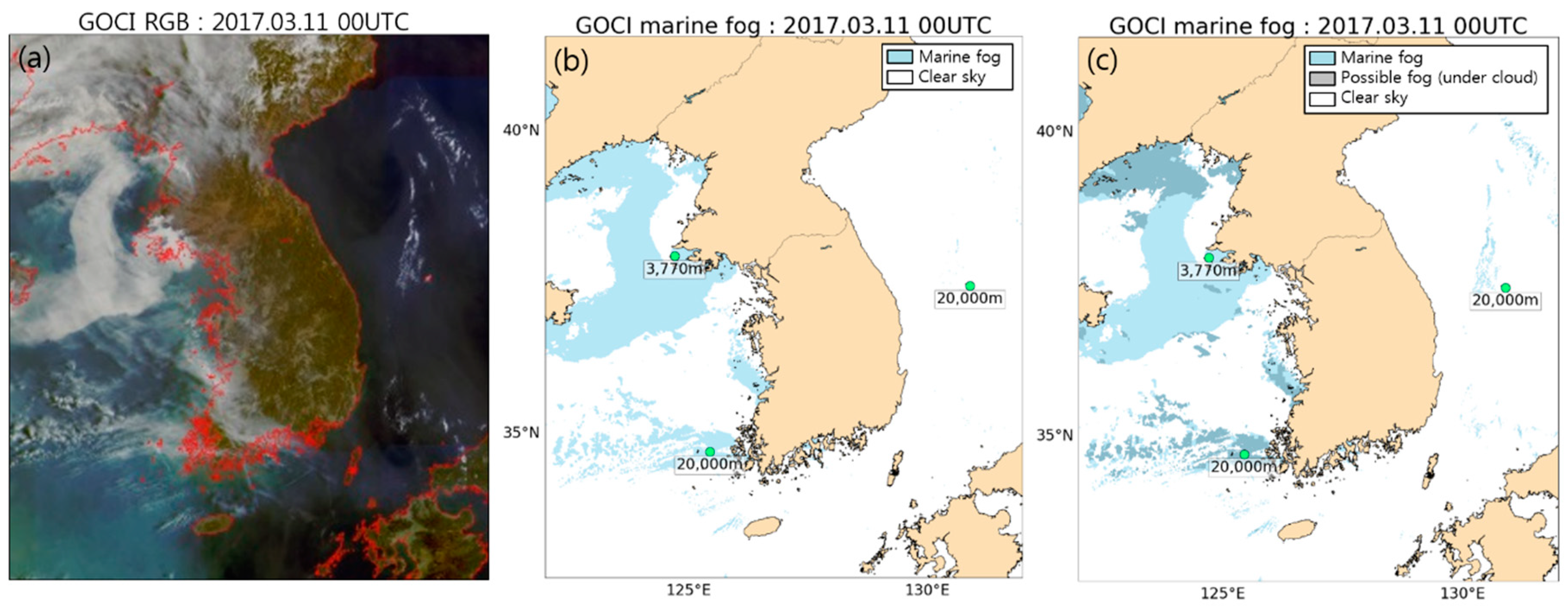
5.1. Validation Using the 2017 Samples

Validation of the algorithm was performed in two ways: using all 2017 MF and nonfog samples and using all but the cases with possible high clouds above the fog. In addition, the homogeneity test was applied. That is, among the pixels within a 2-km radius of the corresponding weather stations, the MF algorithm results (0, 1 or 2) that account for more than 90% of the pixels were identified as representative values. Then, the homogeneous GOCI pixels (a total of 2403 pixels, as listed in

Table 4. Contingency tables for hindcast valid ation (2017) of the developed marine fog detection algorithms: (a) the GOCI-only DT algorithm and (b) after postprocessing.

(a) GOCI-Only DT Algorithm
Validation		Observed		Sum of the forecasts
		“0” Nonfog	“1” Marine fog
Forecast	“0” is nonfog	1020	292	1317
	“1” is marine fog	509	577	1086
	“2” is possible fog (under cloud)	-	-
Sum of the observations		1529	869	2403
Overall accuracy		0.67
Hit rate		0.66
False alarm rate		0.33
(b) After Postprocessing
Validation		Observed		Sum of the forecasts
		“0” Nonfog	“1” Marine fog
Forecast	“0” is nonfog	713	0	713
	“1” is marine fog	327	534	861
	“2” is possible fog (under cloud)	489	335	824
Sum of the observations for all pixels		1529	869	2403
(excluding “2”)		(1040)	(534)	(1574)
Overall accuracy		0.72 (0.79)
Hit rate		0.61 (1.0)
False alarm rate		0.21 (0.31)

) were compared with the visibility data of the corresponding stations.

The validation results of the MF detection algorithm prior to and after the postprocessing stage were compared. Among the 869 real fog pixels, the GOCI-only DT algorithm can correctly detect 577 (HR = 0.66) pixels. In contrast, out of the 1529 nonfog pixels, the algorithm misclassified 509 pixels as fog (FAR = 0.33). The HR increased by including undetected edge regions, but the FAR increased as well (not shown). Implementing the cloud removal procedure by considering the Himawari-8 data (Table 4b) slightly decreased the HR to 0.61, but significantly improved the FAR to 0.21 through the removal of misdetected clouds from the first guess of fog. Accordingly, the postprocessing step increases the overall accuracy from 0.67 to 0.72. Furthermore, by excluding possible high clouds above fog (“2” in Figure 6), 534 real MF pixels were properly detected (HR = 1). As the FAR was 0.31, the overall accuracy reached 0.79.

Figure 9 shows an example of MF detection, which shows that the FAR is reduced in the postprocessing step. On 11 March 2017, the GOCI DT algorithm shows that MF widely occurred across the northern part of the Yellow Sea (Figure 9b), and was rather scattered across the southern part of HS. BN remains just outside of the northern fog detection region, which was in good agreement with the visibility observations (3770 m). HS was located in the middle of the southern scattered fog system (Figure 9b) according to the GOCI-DT-based classification. However, it was changed to “2 (possible cloud)” through postprocessing (Figure 9c). Thus, the final result (e.g., clouds) near the island of HS corresponds well with the high visibility (20,000 m) observations. In summary, the 2017 validation contingency table and the comparison of several retrieval results in the two steps show that the combined use of GOCI and Himawari-8 data is advantageous to the satellite fog detection performance.

5.2. Additional Algorithm Validation

Additional validation of independent 2018 MF cases is performed using in situ visibility data and CALIPSO VFM data.

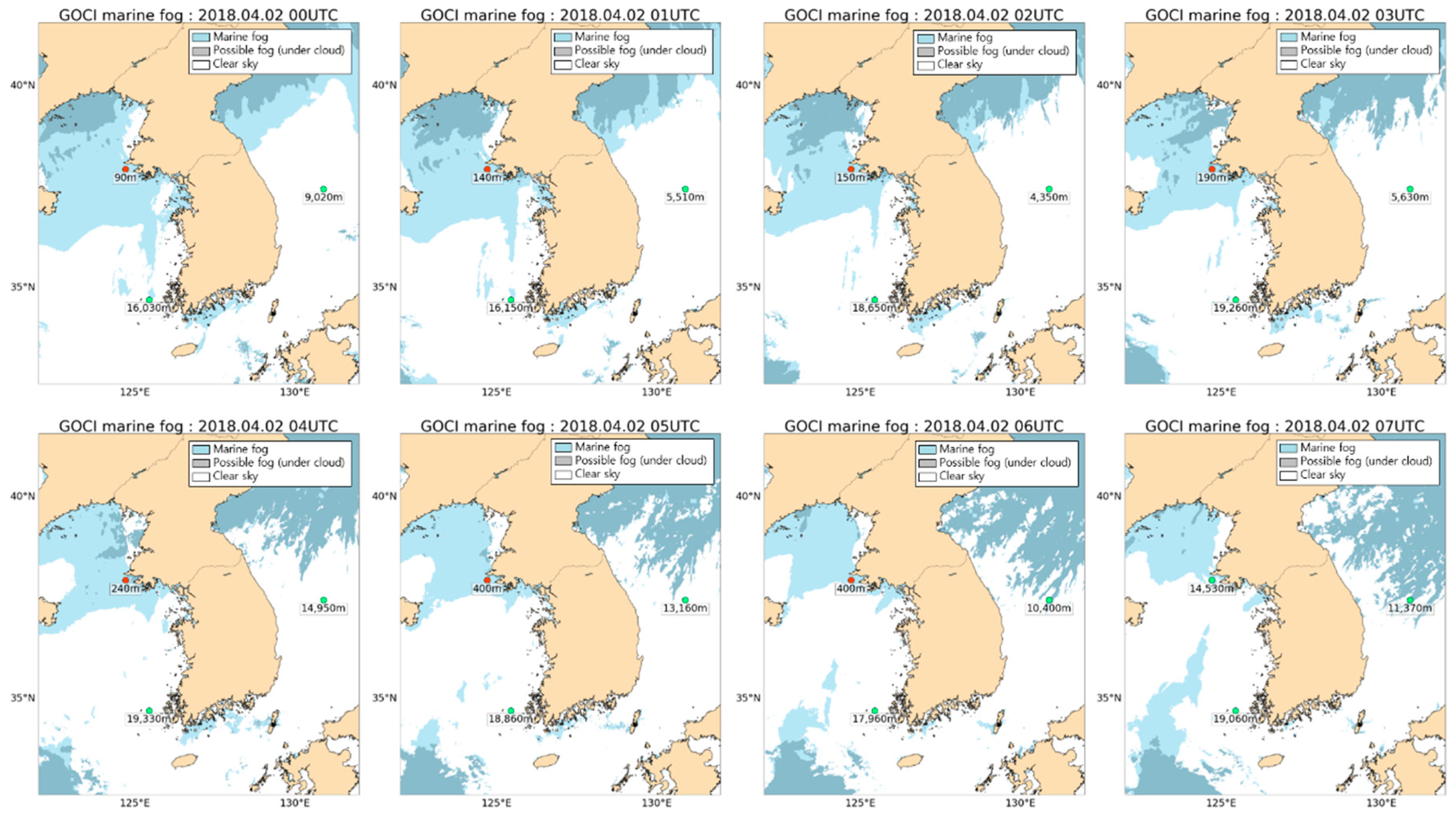
5.2.1. In Situ Visibility Observation

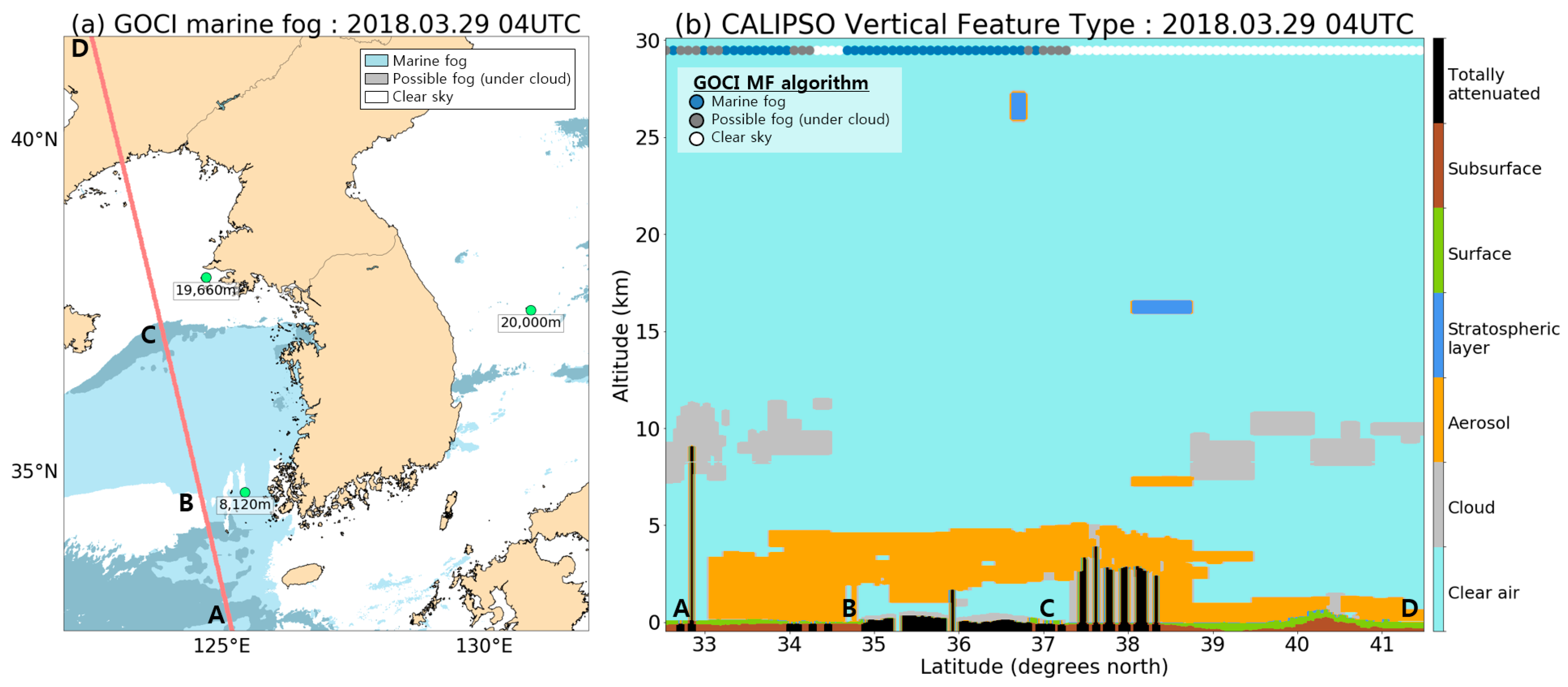
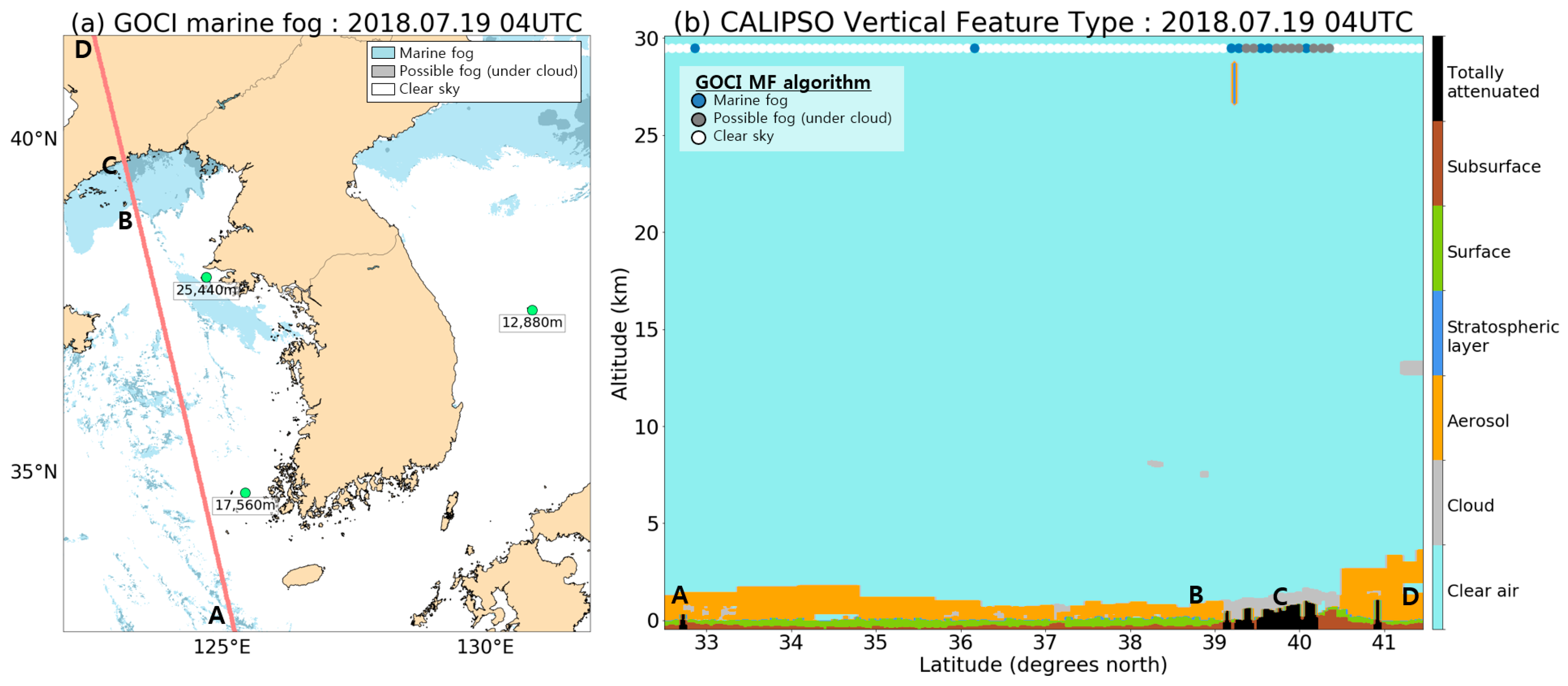
Figure 10 shows the ability of the developed algorithm to capture the hourly MF variability. The results show that the visibility observations at BN indicate the presence of MF, with visibility = 90 m at 00 UTC (09 LT). However, the visibility increased gradually in the daytime, and finally reached 14,540 m at 07 UTC (13 LT). By assessing the location of the BN island station, we can see that the station is continuously located in the middle of the MF from 00 to 06 UTC, and is not in MF at 07 UTC. In contrast, the visibility at the other two stations, which are beyond the fog threshold, is high.

5.2.2. CALIPSO

Because of the absolute lack of in situ MF observations, validation using various platforms was required to further confirm the usefulness of the developed MF algorithm. The CALIPSO VFM data resolve the vertical structure of MF, although only a few MF cases are applicable because of the very narrow footprint (~70 m). Figure 11a and Figure 12a show two MF cases where CALIPSO passes over (red lines) the final MF detection area (sky-blue shading) from the GOCI. The vertical cross-sections on Figure 11b and Figure 12b visualize the feature types derived from the CALIPSO backscatter data for each layer. Light blue, gray, orange and black indicate regions of “clear air”, “cloud”, “aerosol” and “totally attenuated”, respectively. Note that the backscatter signal can be completely attenuated by the overlying layers containing atmospheric particles such as aerosols, opaque clouds and/or stratospheric layers. Some regions directly beneath clouds or MF may exhibit “totally attenuated”.

On 29 March 2018, our developed algorithm shows that MF widely covered the Yellow Sea of South Korea from west of the island of HS to the island of BN along the B‒C line in Figure 11a. Across the East China Sea, cloud pixels are detected in the A‒B region, whose vertical structures by CALIPSO are shown in Figure 11b. Clouds (gray shading) are located near the sea level along the B‒C line. These low-level clouds touching the surface identified by CALIPSO correspond well with the MF detection results of the developed algorithm, as shown in shadings of Figure 11a and dots of Figure 11b. To the south, CALIPSO observed the lifted high clouds located at approximately 7–10 km, which corresponds well with the “possible fog (under clouds)” region by the GOCI MF algorithm in the A‒B region. However, to the southwest of the island of BN, the GOCI algorithm detected a narrow “possible fog (under clouds)” region, which was confirmed as fog by CALIPSO.

Another comparison of CALIOP overpass and MF results is shown in Figure 12a,b for 19 July 2018. Additionally, the MF region retrieved from the MF algorithm (Figure 12a) is consistent with the vertical profile (Figure 12b). In Figure 12b, the very low altitude of clouds (gray shading) along the B‒C line indicates the presence of fog. While only a few cases could be evaluated with CALIPSO, the method using VFM data was very useful to verify MF across a wide area where in situ observations are not available.

6. Summary and Discussion

In this study, a GOCI MF detection algorithm was developed based on the machine learning method for the first time in combination with the Himawari-8 data. The logical relationships and rules between input satellite indices (i.e., GOCI R_rc, NLSD and Himawari CLTH) and the output product (MF “existence”, “no-existence” and “possible fog (under cloud)” classifications for each pixel) were determined through the DT algorithm to utilize the optical and spatial properties of MF (Figure 7). Prior to the development of this algorithm, human subjective decisions based on satellite image analysis procedures (by KIOST KOSC) were required for real-time MF monitoring. The GOCI MF algorithm allows automated fog detection that is available to nonspecialists and is helpful for maritime ship traffic, aviation and coastal ground traffic management.

This algorithm is being used to provide near-real-time MF information in the port oceanographic information system of the Korea Hydrographic and Oceanographic Agency (http://www.khoa.go.kr/pois/popup_seafog.do?lang=en).

In the developed MF algorithm, we were only using visible observations, as the primary input may make our algorithm more stable due to its lower sensitivity to the highly variable environmental conditions (Figure 5). For algorithm development, training (validation) samples were carefully collected through a match-up process between satellite and in situ data (i.e., the KMA station visibility data on the islands of BN, HS and UR). By investigating the optical properties of MF using different satellite variables (Figure 3, Figure 4 and Figure 5), our final algorithm (Figure 6) was designed to use i) the GOCI 412-nm R_rc and its spatial variability index as the main input data and ii) the Himawari-8 CLTH (for supplementary use). Finally, a potential MF region as the first guess is determined through the DT-based rules (Section 4.1), and the detection result is further refined in the postprocessing stage with the CLTH data from Himawari-8 (Section 4.2). Postprocessing consists of cloud removal improvement and fog edge detection (Figure 6).

Unlike a previous study [15], the current GOCI MF algorithm determines thresholds and logical relationships using the machine learning method. Validation using the collected 2017 samples shows a reasonably good performance of the final algorithm (HR = 0.61 and FAR = 0.21). In particular, the combination of GOCI with Himawari-8 data has been used to reduce the FAR (0.33 to 0.21) by improving cloud removal from the first guess of the MF region (Table 4). Real-time validation using the KMA stations (Figure 10) and CALIPSO vertical feature type data (Figure 11 and Figure 12) show that the algorithm suitably detects MF and nonmarine fog regions.

When excluding high clouds above MF, the HR (1.0) is particularly high (Table 4), but the FAR (0.31) became relatively high as well. Such a high FAR can be caused by fine dust, sea ice or stratus clouds, which have similar optical and textural properties as MF. Actually, it is particularly difficult to distinguish MF from stratus clouds. In many cases, fog and low stratus clouds are grouped in the same category [8,14]. It is necessary to remove fine dust or sea ice from the first guess of MF, which will be performed in a future study. Also, the currently trained decision tree is based on observations at three KMA stations in the mid-latitude. Our primary input data (GOCI visible observations) are less dependent on the surface temperature condition; however, we need further investigation if the current MF detection thresholds are applicable to another region.

References

1. Gultepe, I.; Tardif, R.; Michaelides, S.C.; Cermak, J.; Bott, A.; Bendix, J.; Müller, M.D.; Pagowski, M.; Hansen, B.; Ellrod, G.; et al. Fog research: a review of past achievements and future perspectives. Pure Appl. Geophys. 2007, 164, 1121–1159. [Google Scholar] [CrossRef]
2. Tremant, M. La prévision du brouillard en mer. Météorologie Maritime et Activities Océanographique Connexes. WMO 1987, 20, 127. [Google Scholar]
3. Park, J.-M.; Lee, S.M. Greening methods on the back of coastal waterproof wall using halophytes. J. Korean Soc. Fish. Mar. Sci. Educ. 2018, 30, 342–353. [Google Scholar]
4. Scorer, R.S. Cloud Investigation by Satellite; Halstead Press: Chichester, UK; Ellis Horwood: New York, NY, USA, 1986. [Google Scholar]
5. Eyre, J.R. Detection of fog at night using Advanced Very High Resolution Radiometer (AVHRR) imagery. Meteorol. Mag. 1984, 113, 266–271. [Google Scholar]
6. Hunt, G. Radiative properties of terrestrial clouds at visible and infra-red thermal window wavelengths. Q. J. R. Meteorol. Soc. 1973, 99, 346–369. [Google Scholar] [CrossRef]
7. Ellrod, G.P. Advances in the detection and analysis of fog at night using GOES multispectral infrared imagery. Weather Forecast. 1995, 10, 606–619. [Google Scholar] [CrossRef] [Green Version]
8. Cermak, J.; Bendix, J. A novel approach to fog/low stratus detection using Meteosat 8 data. Atmos. Res. 2008, 87, 279–292. [Google Scholar] [CrossRef]
9. Anthis, A.I.; Cracknell, A.P. Use of satellite images for fog detection (AVHRR) and forecast of fog dissipation (METEOSAT) over lowland Thessalia, Hellas. Int. J. Remote Sens. 1999, 20, 1107–1124. [Google Scholar] [CrossRef]
10. Park, H.S.; Kim, Y.H.; Suh, A.S.; Lee, H.H. Detection of fog and the low stratus cloud at night using derived dual channel difference of NOAA/AVHRR data. In Proceedings of the 18th Asian Conference on Remote Sensing, Kuala Lumpur, Malaysia, 20–24 October 1997. [Google Scholar]
11. Lee, J.R.; Chung, C.Y.; Ou, M.L. Fog detection using geostationary satellite data: Temporally continuous algorithm. Asia-Pac. J. Atmos. Sci. 2011, 47, 113–122. [Google Scholar] [CrossRef]
12. Suh, M.S.; Lee, S.J.; Kim, S.H.; Han, J.H.; Seo, E.K. Development of land fog detection algorithm based on the optical and textural properties of fog using COMS data. Korean J. Remote Sens. 2017, 33, 359–375. [Google Scholar]
13. Heo, K.Y.; Kim, J.H.; Shim, J.S.; Ha, K.J.; Suh, A.S.; Oh, H.M.; Min, S.Y. A remote sensed data combined method for sea fog detection. Korean J. Remote Sens. 2008, 24, 1–16. [Google Scholar]
14. Gao, S.H.; Wu, W.; Zhu, L.; Fu, G. Detection of nighttime sea fog/stratus over the Huang-hai Sea using MTSAT-1R IR data. Acta Oceanol. Sin. 2009, 28, 23–35. [Google Scholar]
15. Yuan, Y.; Qiu, Z.; Sun, D.; Wang, S.; Yue, X. Daytime sea fog retrieval based on GOCI data: a case study over the Yellow Sea. Opt. Express 2016, 24, 787–801. [Google Scholar] [CrossRef] [PubMed]
16. Friedl, M.A.; Brodley, C.E. Decision tree classification of land cover from remotely sensed data. Remote Sens. Env. 1997, 61, 399–409. [Google Scholar] [CrossRef]
17. Park, M.S.; Kim, M.; Lee, M.I.; Im, J.; Park, S. Detection of tropical cyclone genesis via quantitative satellite ocean surface wind pattern and intensity analyses using decision trees. Remote Sens. Environ. 2016, 183, 205–214. [Google Scholar] [CrossRef]
18. Kim, M.; Park, M.S.; Im, J.; Park, S.; Lee, M. Machine Learning Approaches for Detecting Tropical Cyclone Formation Using Satellite Data. Remote Sens. 2019, 11, 1195. [Google Scholar] [CrossRef] [Green Version]
19. Ahn, J.H.; Park, Y.J.; Ryu, J.H.; Lee, B.; Oh, I.S. Development of Atmospheric Correction Algorithm for Geostationary Ocean Color Imager (GOCI). Ocean Sci. J. 2012, 47, 247–259. [Google Scholar] [CrossRef]
20. Choi, J.K.; Park, Y.J.; Ahn, J.H.; Lim, H.S.; Eom, J.; Ryu, J.H. GOCI, the world’s first geostationary ocean color observation satellite, for the monitoring of temporal variability in coastal water turbidity. J. Geophys. Res.-Ocean. 2012, 117. [Google Scholar] [CrossRef]
21. Choi, M.; Kim, J.; Lee, J.; Kim, M.; Park, Y.J.; Jeong, U.; Song, C.H. GOCI Yonsei Aerosol Retrieval (YAER) algorithm and validation during the DRAGON-NE Asia 2012 campaign. Atmos. Meas. Tech. 2016, 9, 1377–1398. [Google Scholar] [CrossRef] [Green Version]
22. Gordon, H.R.; Brown, J.W.; Evans, R.H. Exact Rayleigh scattering calculations for use with the Nimbus-7 coastal zone color scanner. Appl. Opt. 1988, 27, 862–871. [Google Scholar] [CrossRef]
23. Gordon, H.R.; Wang, M. Surface-roughness considerations for atmospheric correction of ocean color sensors. 1: The Rayleigh-scattering component. Appl. Opt. 1992, 31, 4247–4260. [Google Scholar] [CrossRef] [PubMed]
24. Wang, M. The Rayleigh lookup tables for the SeaWiFS data processing: Accounting for the effects of ocean surface roughness. Int. J. Remote Sens. 2002, 23, 2693–2702. [Google Scholar] [CrossRef]
25. Wang, M. A refinement for the Rayleigh radiance computation with variation of the atmospheric pressure. Int. J. Remote Sens. 2005, 26, 5651–5663. [Google Scholar] [CrossRef]
26. Wang, M. Rayleigh radiance computations for satellite remote sensing: Accounting for the effect of sensor spectral response function. Opt. Express 2016, 24, 12414–12429. [Google Scholar] [CrossRef]
27. Bessho, K.; Date, K.; Hayashi, M.; Ikeda, A.; Imai, T.; Inoue, H.; Okuyama, A. An introduction to Himawari-8/9—Japan’s new-generation geostationary meteorological satellites. J. Meteorol. Soc. Jpn. Ser. Ii 2016, 94, 151–183. [Google Scholar] [CrossRef] [Green Version]
28. KMA. Meteorological Information Portal Service System. 2017. Available online: http://afso.kma.go.kr (accessed on 1 June 2019).
29. Vaisala, 2010: User’s guide-Vaisala Present Weather Detec-tor PWD22/52, 210543EN-D. Available online: https://www.vaisala.com/en/products/instruments-sensors-and-other-measurement-devices/weather-stations-and-sensors/pwd22-52 (accessed on 30 December 2019).
30. WMO. Guide to Meteorological Instruments and Methods of Observation; 6 edition WMO-No. 8; World Meteorological Organisation: Geneva, Switzerland, 2008; 716p. [Google Scholar]
31. Winker, D.M.; Pelon, J.; Coakley, J.A., Jr.; Ackerman, S.A.; Charlson, R.J.; Colarco, P.R.; Flamant, P.; Fu, Q.; Hoff, R.M.; Kittaka, C.; et al. The CALIPSO Mission: A Global 3D View of Aerosols and Clouds. Bull. Am. Meteorol. Soc. 2010, 91, 1211–1229. [Google Scholar] [CrossRef]
32. Quinlan, J.R. Induction of decision trees. Mach. Learn. 1986, 1, 81–106. [Google Scholar] [CrossRef] [Green Version]
33. Mather, P.; Tso, B. Classification Methods for Remotely Sensed Data; CRC Press: Boca Raton, FL, USA, 2016. [Google Scholar]
34. Han, H.; Lee, S.; Im, J.; Kim, M.; Lee, M.I.; Ahn, M.; Chung, S.R. Detection of convective initiation using Meteorological Imager onboard Communication, Ocean, and Meteorological Satellite based on machine learning approaches. Remote Sens. 2015, 7, 9184–9204. [Google Scholar] [CrossRef] [Green Version]
35. Breiman, L.; Friedman, J.H.; Olshen, R.A.; Stone, C.I. Classification and Regression Trees; Chapman & Hall/CRC: Boca Raton, FL, USA, 1984. [Google Scholar]
36. Houze, R.A. Cloud Dynamics, 53th ed.; Academic Press: San Diego, CA, USA, 1993; p. 137. [Google Scholar]
Figure 1. Examples of the Geostationary Ocean Color Imager (GOCI) red, green, blue (RGB) images of marine fog cases. These fog cases were selected through analysis of GOCI RGB images.
Remotesensing 12 00149 g001
Figure 2. Locations and names of the Korean Meteorological Administration (KMA) weather stations on the islands (Baengnyeong (BN), Heuksan (HS) and Ulreung (UR)).
Remotesensing 12 00149 g002
Figure 3. Input variables used for the marine fog detection algorithm: (a) GOCI Rrc, (b) normalized local standard deviation (NLSD) of GOCI Rrc and (c) Himawari-8 cloud top height (CLTH) for April 14, 2016. The red, yellow and green boxes indicate marine fog, low-level cloud and high-level cloud regions, respectively.
Remotesensing 12 00149 g003
Figure 4. R rc distribution of mid-/high-level cloud and marine fog samples in each GOCI band. The red and blue bars indicate the normalized numbers of clouds and marine fog, respectively.
Remotesensing 12 00149 g004
Figure 5. Histogram of the GOCI (a, d) R rc , (b,e) NLSD and (c,f) Himawari-8 IR values of the marine fog samples. Relatively cold (ac) and warm (df) months are displayed separately.
Remotesensing 12 00149 g005
Figure 6. Flow chart of the final marine fog detection algorithm.
Remotesensing 12 00149 g006
Figure 7. Schematic of the decision tree structure of the marine fog detection algorithm.
Remotesensing 12 00149 g007
Figure 8. GOCI RGB image (a), the results of the marine fog detection algorithm before postprocessing (b), algorithm with postprocessing of cloud removal (c) and additional edge detection (d) using the Himawari-8 CLTH data.
Remotesensing 12 00149 g008
Figure 9. (a) GOCI RGB image and marine fog detection image obtained from the GOCI marine fog detection algorithm (b) without and (c) with postprocessing on 2017.03.11 at 00 UTC. The white and sky-blue areas indicate clear-sky sea and marine fog regions, respectively, and the gray area is the region with clouds or marine fog under clouds. The numbers below the marks are the observed visibility at each station. In addition, the color of the filled circle at the stations is red with a visibility less than 1 km, but green with a visibility greater than 1 km.
Remotesensing 12 00149 g009
Figure 10. Validation of the GOCI marine fog detection algorithm on 2018.04.02 with the visibility data obtained at the KMA weather stations. The shadings and circle marks have the same meaning as in Figure 9.
Remotesensing 12 00149 g010
Figure 11. Evaluation of the GOCI marine fog detection algorithm on 29 March 2018 at 04 UTC with Cloud-Aerosol Lidar and Infrared Pathfinder Satellite Observation Vertical Feature Mask (CALIPSO VFM) data. In the left panel (a), the shadings and circle marks have the same meaning as in Figure 9, and the red line represents the Cloud-Aerosol Lidar with Orthogonal Polarization (CALIOP) trajectory. The vertical profile along these footprint lines is shown in the right panel (b). Seven types of features are displayed in different colors at altitudes from 0 to 30 km. Light blue, gray, orange and black indicate clear air, cloud, aerosol and totally attenuated regions, respectively. Colors of the dots at the 30 km altitude represent classified result of the GOCI MF algorithm as shadings in (a). The white, sky-blue and gray dots indicate clear-sky sea, marine fog and possible fog under the clouds, respectively, at the corresponding latitude.
Remotesensing 12 00149 g011
Figure 12. Validation of the GOCI marine fog detection algorithm on 19 July 2018 at 04 UTC with CALIPSO VFM data. The shadings and circle marks have the same meaning as in Figure 11.
Remotesensing 12 00149 g012