Object Detection in Remote Sensing Images Based on Improved Bounding Box Regression and Multi-Level Features Fusion

Abstract

The objective of detection in remote sensing images is to determine the location and category of all targets in these images. The anchor based methods are the most prevalent deep learning based methods, and still have some problems that need to be addressed. First, the existing metric (i.e., intersection over union (IoU)) could not measure the distance between two bounding boxes when they are nonoverlapping. Second, the exsiting bounding box regression loss could not directly optimize the metric in the training process. Third, the existing methods which adopt a hierarchical deep network only choose a single level feature layer for the feature extraction of region proposals, meaning they do not take full use of the advantage of multi-level features. To resolve the above problems, a novel object detection method for remote sensing images based on improved bounding box regression and multi-level features fusion is proposed in this paper. First, a new metric named generalized IoU is applied, which can quantify the distance between two bounding boxes, regardless of whether they are overlapping or not. Second, a novel bounding box regression loss is proposed, which can not only optimize the new metric (i.e., generalized IoU) directly but also overcome the problem that existing bounding box regression loss based on the new metric cannot adaptively change the gradient based on the metric value. Finally, a multi-level features fusion module is proposed and incorporated into the existing hierarchical deep network, which can make full use of the multi-level features for each region proposal. The quantitative comparisons between the proposed method and baseline method on the large scale dataset DIOR demonstrate that incorporating the proposed bounding box regression loss, multi-level features fusion module, and a combination of both into the baseline method can obtain an absolute gain of 0.7%, 1.4%, and 2.2% or so in terms of mAP, respectively. Comparing this with the state-of-the-art methods demonstrates that the proposed method has achieved a state-of-the-art performance. The curves of average precision with different thresholds show that the advantage of the proposed method is more evident when the threshold of generalized IoU (or IoU) is relatively high, which means that the proposed method can improve the precision of object localization. Similar conclusions can be obtained on a NWPU VHR-10 dataset.

1. Introduction

Great progress made on remote sensing technologies means that a large number of remote sensing images (RSIs) with high spatial or spectral resolution are available. Thus, the valuable information represented in RSIs requires better analysis methods to meet the needs of many military and civilian applications [1]. These applications may consist of multiple tasks such as scene classification [2,3,4], object detection [5,6], and other tasks [7,8,9,10]. The goal of object detection in remote sensing images (ODRSIs) is to determine the locations of objects of interest and then to predict their classes. Due to its vital role in surveillance, fire prevention, urban planning, and other tasks, ODRSIs have attracted increasing attention [11,12,13].

In the early stages, handcrafted-based features such as scale invariant feature transform (SIFT) [14], bag of words (BoW) [15], histogram of oriented gradient (HOG) [16], deformable part model (DPM) [17], etc. were employed by many object detection methods in RSIs. Later, shallow learning algorithms such as spatial sparse coding [18], independent component analysis (ICA) [19], etc. quickly gained a modest degree of application in ODRSIs. Recently, significant progress has been made on deep learning techniques [20,21,22,23], meaning the deep learning based methods now significantly outperform handcrafted features and shallow learning based methods. At present, the most prevalent deep learning based methods are anchor-based methods, which can be roughly classified into one-stage and two-stage methods according to their strategy for generating proposals.

The one-stage methods, also called region-free methods, yield a series of grid-based bounding boxes for prediction. You only look once (YOLO) [24], which accomplishs the object detection through a regression strategy, divided the input image into separate parts and predicted the category of each part. YOLO v2 [25] and YOLO v3 [26], which are the subsequent improved methods of YOLO, attracted more widespread attention. Another classical one-stage method called single shot multibox detector (SSD) [27] generates a series of prior boxes with different scales and aspect ratios across multiple feature maps, and predicts the category of each box. Due to the fast detection speed, the one-stage methods have been applied to ODRSIs. Liu et al. [28] proposed an ODRSIs method based on the YOLOv2 framework, which combined the multi-level features and used a feature introducing scheme to enhance the accuracy of small-scale object detection. To improve the computation efficiency and the effect of small object detection, Chen et al. [29] incorporated the semantic segmentation and global activation information into the SSD framework for object detection in RSIs. The other works examining ODRSIs based on one-stage methods include Tang et al. [30], Tayara et al. [31], and Chen et al. [32].

Although one-stage methods achieve high detection speeds, their detection accuracy is lower than that of two-stage methods. Consequently, more researchers focus on the two-stage methods, i.e., region proposals based methods, which firstly generate region proposals via a region proposal network (RPN) and then conduct bounding box regression and classification for each proposal. The canonical two-stage methods, such as Faster R-CNN [33], Region-based Fully Convolutional Networks (R-FCN) [34], and feature pyramid network (FPN) [35], have a substantial influence on ODRSIs. For example, Li et al. [36] incorporated additional multi-angle anchors into RPN for solving the rotational variations of object, and it also introduced a local-contextual feature fusion module to alleviate the problem of appearance ambiguities for ODRSIs. Zhong et al. [37] proposed a position-sensitive strategy to improve the detection speed by sharing the most computation on the entire image. Chen et al. [38] used the ResNeXt [39] as the backbone and incorporated scene-contextual information into FPN, moreover, they utilized group normalization (GN) [40] as an alternative to batch normalization (BN) [41].

However, there are some common problems in both one-stage and two-stage methods. On the one hand, the existing bounding box regression loss cannot directly optimize the metric (i.e., IoU) in ODRSIs. Specifically, there is no direct correlation between the existing bounding box regression loss (i.e., smooth L1 loss [33] and L2 loss [42]) and IoU. It is worth noting that designing a bounding box regression loss based on IoU is not suitable because the IoU can not quantify the distance between two bounding boxes when they are nonoverlapping. As a matter of fact, if two bounding boxes are nonoverlapping, the IoU is always zero no matter how far away the two bounding boxes are. Although the generalized intersection over union (GIoU) loss [43] has been proposed in natural image object detection to alleviate the problem mentioned above, the effect is restricted due to the constant gradient of bounding box regression (the details can be seen in Section 2.1.3).

On the other hand, the existing methods which adopt a hierarchical deep network have several problems in the feature extraction of region proposals. In existing methods, the RPN firstly generates a large number of region proposals from all the layers. Next, the size of each region proposal is quantified to determine the feature level to which the proposals belong. Finally, the features of each region proposal are extracted from the selected feature level. Obviously, this approach has two problems: (1) two proposals with similar sizes are likely to be assigned to different levels due to quantization error; (2) each proposal just maps to a single feature map, which does not make full use of the advantages of multi-level features. In fact, the multi-level features are used only at the RPN stage and are not considered during the subsequent feature extraction of region proposals.

To resolve the above problems, a novel ODRSIs method based on improved bounding box regression and multi-level features fusion is proposed in this paper. First, a new metric named GIoU [43] is introduced, which can tackle both overlapping and nonoverlapping cases between two bounding boxes. This solves the problem that existing metrics (i.e., IoU) fail to measure the distance for the nonoverlapping cases for ODRSIs. Then, to solve the problem that the existing bounding box regression loss could not directly optimize the metric in ODRSIs, a new bounding box regression loss named IGIoU loss is proposed, which can optimize the new metric (i.e., GIoU) directly and solve the aforementioned constant gradient problem involving GIoU loss [43]. Furthermore, a multi-level features fusion (MLFF) module is proposed to combine the multi-level features for each proposal to overcome the weakness of multi-level features methods not make full use of all available advantages.

The main contributions of this paper are as follows:

(1)

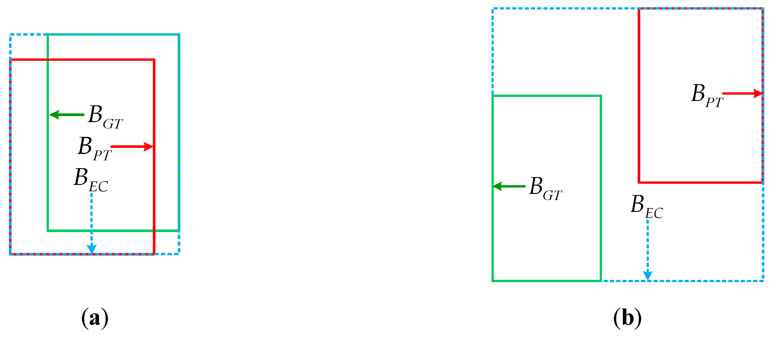
A new metric (i.e., GIoU) for ODRSIs is adopted to replace the existing metric (i.e., IoU). The GIoU overcomes the problem that the IoU cannot measure the distance when the predicted bounding box and the ground truth box are nonoverlapping.

(2)

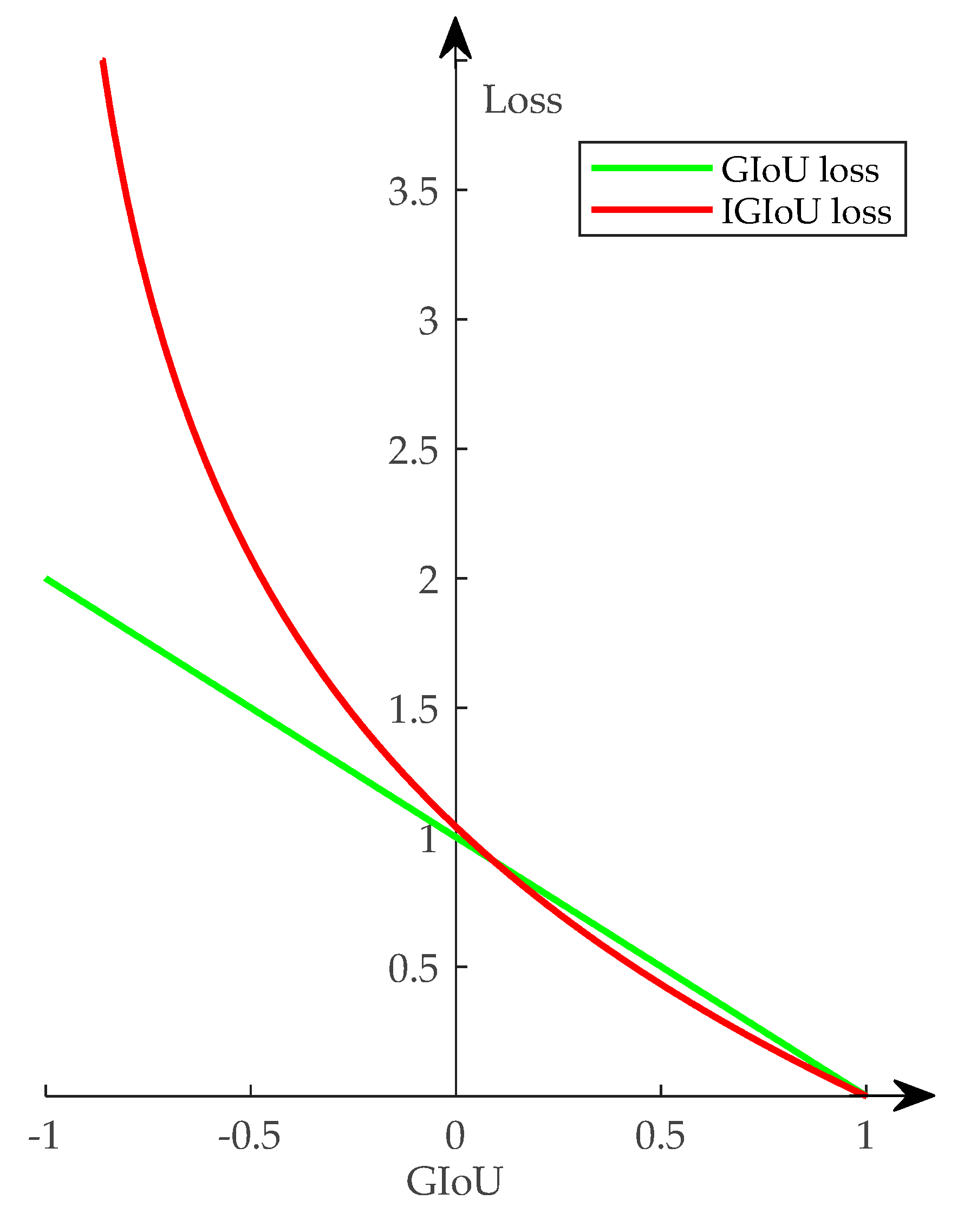
A novel bounding box regression loss named IGIoU loss is proposed. The proposed IGIoU loss can optimize the new metric (i.e., GIoU) directly, which thus solves the problem that the existing bounding box regression loss cannot directly optimize the metric in ODRSIs. Furthermore, it can overcome the problem that existing GIoU loss [43] cannot adaptively change the gradient based on the GIoU value.

(3)

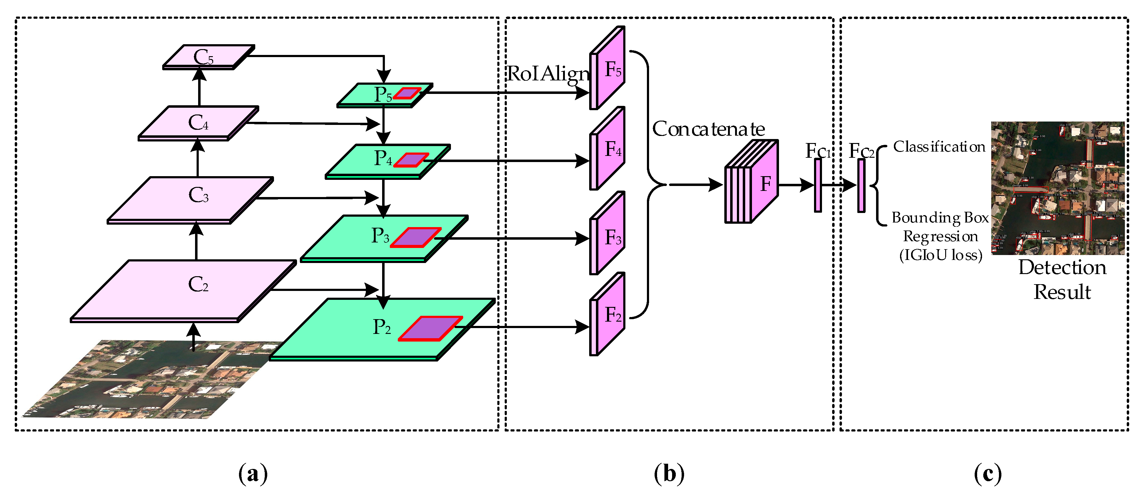
A multi-level features fusion module named MLFF module is proposed. The proposed MLFF can be incorporated into the existing hierarchical deep network, which can address the problem that the existing methods which adopt a hierarchical deep network do not make full use of the advantages of multi-level features for the feature extraction of region proposals.

2. Materials and Methods

2.1. Methods

The overall architecture of our method is illustrated in Figure 1. First, given a remote sensing image with an arbitrary size as an input, the FPN was adopted as the backbone network, which yields multi-scale feature maps at different levels. Next, the obtained multi-scale feature maps were fed into an MLFF module, which pools features via RoIAlign [44] (i.e., an alternative to RoI pooling [33]) across levels $p_2$ to $p_5$ for each proposal and then fuses them by concatenating the pooled features along the channel dimension. Finally, the fused features of each proposal were utilized for bounding box regression and classification. Note that our IGIoU loss was adopted to replace the smooth L1 loss used in the original FPN for bounding box regression.

2.1.1. Multi-Level Features Fusion

In the original FPN, each proposal generated from RPN was mapped back to a kth level feature map (i.e., $P_k$ in Figure 1a) and multi-level feature maps based on the size of the proposal. The level k was defined by:

$$k=\lfloor k_0+lo{g}_2(\sqrt{wh}/224)\rfloor$$

(1)

where $\lfloor \cdot \rfloor$ denotes the rounding down operation, $w$ and $h$ separately represent the width and height of the proposal, $k_0$ was the level corresponding to the proposal with $wh={224}^2$, $224 \times 224$ was the size of the input layer of ResNet50 (the backbone network). The default value of $k_0$ was 4, which is analogous to Faster R-CNN with a ResNet backbone that employs $C_4$ as a single-scale feature map.

As shown in Equation (1), the smaller proposals were assigned to lower levels. Similarly, the larger proposals were assigned to higher levels. However, there were some problems for this assigning scheme, for instance, the proposals with similar size were possibly assigned to different level feature maps because of the quantization error of Equation (1). Furthermore, the advantages of the hierarchical features representation of FPN were not fully utilized since the feature of every proposal was only extracted from the single level feature map of FPN.

A MLFF module is proposed in this paper to tackle the aforementioned problems. The framework of MLFF is given in Figure 1b. The feature maps of all levels (i.e., $P_2\sim P_5$) were used by a MLFF module for feature extraction of each proposal. The details of the MLFF module are presented as follows.

First of all, each proposal generated by the RPN was mapped back to the feature maps across all levels, which were denoted by pink regions throughout all levels in Figure 1a. The size and spatial location of any pink region in each level feature map can be calculated based on the size ratio between the proposal and feature maps. The top-left and right-down coordinates of any pink region in ith level feature map can be obtained by using the following equations:

$$\begin{array}{l}{x}_i^{TL}=Round(p^{TL}\times \frac{w_i}{w_{img}}),\hspace{0.17em}{y}_i^{TL}=Round(q^{TL}\times \frac{h_i}{h_{img}})\\ x_i^{RD}=Round(p^{RD}\times \frac{w_i}{w_{img}}),\hspace{0.17em}{y}_i^{RD}=Round(q^{RD}\times \frac{h_i}{h_{img}})\end{array}, i\in [2,5]$$

(2)

where $(x_i^{TL},y_i^{TL})$ and $(x_i^{RD},y_i^{RD})$ denote the top-left and right-down coordinates of any pink region in an ith level feature map, respectively, $(p^{TL},q^{TL})$ and $(p^{RD},q^{RD})$ denote the top-left and right-down coordinates of region proposals in the input image, respectively, $(w_{img},h_{img})$ denotes the width and height of the input image, $(w_i,h_i)$ denotes the width and height of the ith level feature map, and $Round(\cdot )$ denotes the rounding operation.

Afterwards, the four level pink regions of each proposal were transformed into four groups of 7 × 7 feature maps (denoted as F₂, F₃, F₄, and F₅, as shown in Figure 1b) through the RoIAlign operation [44], and the fused features of each proposal can be obtained by the following equation:

$$F=F_2\oplus F_3\oplus F_4\oplus F_5$$

(3)

where F denotes the fused features of each proposal and $\oplus$ denotes the concatenation operation along channel dimension.

The convolutional operation with 7 × 7 kernel was imposed on $F$ to obtain the FC₁, and the FC₁ was followed by a fully connected layer (i.e., FC₂) for bounding box regression and classification.

2.1.2. Generalized Intersection over Union

The IoU is a normalized measure which was adopted for evaluating the proximity of two bounding boxes. The IoU was insensitive to the scales of the bounding boxes and has been widely used to ODRSIs. As shown in Figure 2, the IoU between ground truth box $B_{GT}$ and predicted bounding box $B_{PT}$ can be calculated as follows:

$$\mathrm{IoU}=\frac{area(B_{GT}\cap B_{PT})}{area(B_{GT}\cup B_{PT})}, \mathrm{IoU}\in [0,1]$$

(4)

where $area(B_{GT}\cap B_{PT})$ and $area(B_{GT}\cup B_{PT})$ denote the area of intersection and union between $B_{GT}$ and $B_{PT}$ respectively. Note that IoU was suitable for evaluating the proximity of two bounding boxes shown in Figure 2a, however, the $area(B_{GT}\cap B_{PT})$ was always zero in the case shown in Figure 2b. In other words, the IoU could not measure the distance when two bounding boxes were nonoverlapping. In this paper, a new metric (i.e., GIoU) was adopted to address this problem. The definition of GIoU was given as follows:

$$\mathrm{GIoU}=\mathrm{IoU}+\frac{area(B_{GT}U{B}_{PT})}{area(B_{EC})}-1, \mathrm{GIoU}\in (-1,1]$$

(5)

where $B_{EC}$ and $area(B_{EC})$ denote the smallest enclosing box of $B_{GT}$ and $B_{PT}$ and its area, respectively. As shown in Figure 2, the IoU was inversely proportional to the distance between $B_{GT}$ and $B_{PT}$ when they were overlapping, and the IoU remained at zero when the they were nonoverlapping. In contrast, the $area(B_{EC})$ was always proportional to the distance of two bounding boxes. In summary, as shown in Equation (5), the GIoU monotonously decreased with the distance between $B_{GT}$ and $B_{PT}$, regardless of whether or not the two bounding boxes were overlapping. Apparently, the GIoU can overcome the aforementioned shortcoming of IoU.

2.1.3. Bounding Box Regression Based on IGIoU Loss

The bounding box regression loss of existing object detection methods in RSIs is usually adopted to smooth L1 or L2 loss. Despite this, the two loss functions do not directly optimize the metric. Specifically, the smooth L1 or L2 loss is used to optimize the four independent parameters of the predicted bounding box, while the IoU emphasizes the overlapping degree between two bounding boxes. Therefore, it was necessary to adopt a more reasonable loss function to perform the bounding box regression.

Incorporating the IoU into bounding box regression loss was a logical consideration. However, as mentioned in the last section, the IoU remains zero when two bounding boxes are nonoverlapping, and the bounding box regression cannot be implemented in this case if a IoU based loss function is adopted. Therefore, designing the bounding box regression loss function based on IoU was impractical.

To address this problem, Rezatofighi et al. [43] propose a GIoU loss in natural image object detection, which incorporates the GIoU into the bounding box regression loss. The formulation of GIoU loss was given as follows:

$$L_{\mathrm{GIoU}}=1-\mathrm{GIoU}$$

(6)

where $L_{\mathrm{GIoU}}$ denotes the GIoU loss, and the curve of $L_{\mathrm{GIoU}}$ is shown in Figure 3. Obviously, the GIoU loss can alleviate the aforementioned shortage which existed in IoU based loss by directly optimizing the metric (i.e., GIoU). However, as shown in Figure 3, the GIoU loss has a constant gradient during the whole training process, which restricts the effect of bounding box regression to some extent. As a matter of fact, the strength of training should be enhanced when the predicted bounding box is far away from the ground truth box. In other words, the absolute value of the gradient should be increased when the GIoU is small. In addition, the value of the bounding box regression loss should decrease with the GIoU. Following above analysis, an improved GIoU loss (IGIoU loss) was proposed for the bounding box regression in this paper. The formulation of IGIoU loss was given as follows:

$$L_{\mathrm{IGIoU}}=2\times log2-2\times log(1+\mathrm{GIoU})$$

(7)

where $L_{\mathrm{IGIoU}}$ denotes the IGIoU loss. The curve of $L_{\mathrm{IGIoU}}$ is also shown in Figure 3 for intuitive comparison between the GIoU loss and IGIoU loss.

As shown in Figure 3, both $L_{\mathrm{IGIoU}}$ and $L_{\mathrm{GIoU}}$ monotonously decrease with GIoU, the absolute value of gradient of $L_{\mathrm{IGIoU}}$ also monotonously decreases with GIoU, and the gradient of $L_{\mathrm{GIoU}}$ does not change with GIoU. Apparently, the use of IGIoU is better for bounding box regression. Specifically, the larger absolute value of a gradient is required when the distance between predicted bounding boxes and ground truth bounding boxes is large (i.e., GIoU is small). As shown in Figure 3, the absolute value of gradient of $L_{\mathrm{IGIoU}}$ is larger than that of $L_{\mathrm{GIoU}}$ when GIoU is small, which coincides with the above analysis. A similar conclusion can be derived when GIoU was large. In summary, the designing of $L_{\mathrm{IGIoU}}$ was more reasonable than $L_{\mathrm{GIoU}}$ from the perspective of theoretical analysis.

2.2. Experimental Materials

2.2.1. Dataset

To validate the effectiveness of our method, various experiments on the NWPU VHR-10 [42,45,46] and DIOR benchmark dataset were conducted with a total of 3775 instances and 192,472 instances available, respectively. The details of both datasets are listed in Figure 4.

The NWPU VHR-10 dataset includes 800 very-high-resolution RSIs acquired from Vaihingen datasets [47] and Google Earth. The dataset was divided into two parts: one was a positive set that includes 650 images, each of which covered at least one of the 10 categories, with some examples listed in Figure 5: (a) airplane, (b) baseball diamond, (c) basketball court, (d) bridge, (e) ground track field, (f) harbor, (g) ship, (h) storage tank, (i) tennis court, and (j) vehicle. The other one was a negative set including 150 images that did not contain any objects belonging to the above categories. The negative set was intended for weakly supervised learning methods [48] or semi-supervised learning methods [49]. Therefore, the negative set was not utilized in our experiments. The positive set was divided into training, validation, and testing sets, which include 20%, 20%, and 60% of the images of the positive set, respectively [37,42].

Considering the fact that the number of the samples of the NWPU VHR-10 dataset is limited, the DIOR dataset recently proposed by Li et al. [50] was also utilized to verify the effectiveness and generalization of the proposed method in this paper. The DIOR dataset is a large scale benchmark, the size of which is comparable to another well-known large-scale DOTA dataset [51,52]. Specifically, the DIOR dataset includes 23,463 images and 192,472 object instances covered by 20 categories, where each category contains around 1200 images. The 20 categories cover all categories in the NWPU VHR-10 dataset as well as other ten categories, with some examples listed in Figure 5: (k) airport, (l) chimney, (m) dam, (n) expressway service area, (o) expressway toll station, (p) golf course, (q) overpass, (r) stadium, (s) train station, and (t) wind mill. The training set, validation set, and testing set include 5862 images, 5863 images, and 11,738 images, respectively [50].

2.2.2. Evaluation Metrics

The evaluation metrics adopted by this paper were similar to the metrics used on MS COCO [53]. Specifically, the average precision (AP) under multiple thresholds and mean average precision (mAP) were adopted to quantitatively evaluate the experimental results. Note that both GIoU and IoU were utilized as metrics to comprehensively demonstrate the advantages of our method, which include:

(1) The ability to determine the curve of AP with a different threshold. The AP was calculated by using the area under the precision-recall curve (p-r curve) [54,55,56]. The precison and recall were defined as follows:

$$\mathrm{Precision}=\frac{TP}{TP+FP}$$

(8)

$$\mathrm{Recall}=\frac{TP}{TP+FN}$$

(9)

where $TP$, $FP$, and $FN$ separately represent the number of true positives, false positives, and false negatives, respectively. Obviously, the precision denotes the ratio of correctly detected results (i.e., true positives) out of all the detected results, and the recall denotes the ratio of true positives that were correctly detected. The detection result was considered to be a true positive when the metric (i.e., GIoU or IoU) exceeded a fixed threshold, otherwise it was treated as false positive. Obviously, the value of AP was changed with different thresholds. Therefore, the curve of AP with a different threshold (i.e., 0.5–0.95) was adopted for comprehensively evaluating the effectiveness of our method, as shown in Figure 6, Figure 7, Figure 8 and Figure 9.

(2) mAP. In general, the AP50 denotes the AP value when threshold was 0.5, meaning the definitions of AP55, ..., AP90, and AP95 are similar to AP50. The mAP is the mean value of AP50–AP95. The mAP, AP50, and AP75 were utilized for quantitative evaluation of our method, as shown in

Table 1. Comparison with baseline methods on NWPU VHR-10 dataset in terms of six evaluation metrics. Bold fonts denote the best results.

Method	GIoU			IoU
	mAP (%)	AP50 (%)	AP75 (%)	mAP (%)	AP50 (%)	AP75 (%)
FPN(baseline)	55.3	88.8	64.0	56.5	89.3	65.9
FPN+MLFF	56.2	89.6	64.2	57.5	90.4	66.7
FPN+GIoU	56.2	88.9	65.9	57.5	89.3	67.5
FPN+IGIoU	57.3	89.8	66.6	58.5	90.7	68.5
FPN+MLFF+GIoU	57.0	89.5	66.1	58.2	90.8	67.8
FPN+MLFF+IGIoU(Ours)	58.0	90.5	67.5	59.2	91.4	69.6

,

Table 2. Comparison with four state-of-the-art methods on NWPU VHR-10 dataset in terms of six evaluation metrics. Bold fonts denote the best results.

Method	GIoU			IoU
	mAP (%)	AP50 (%)	AP75 (%)	mAP (%)	AP50 (%)	AP75 (%)
Faster R-CNN	53.5	86.8	61.0	54.6	87.1	62.6
Mask R-CNN	54.7	88.8	62.6	55.8	89.4	64.2
FPN	55.3	88.8	64.0	56.5	89.3	65.9
PANet	56.3	90.5	63.9	57.8	91.8	65.8
Ours	58.0	90.5	67.5	59.2	91.4	69.6

,

Table 3. Comparison with baseline methods on the DIOR dataset in terms of six evaluation metrics. Bold fonts denote the best results.

Method	GIoU			IoU
	mAP (%)	AP50 (%)	AP75 (%)	mAP (%)	AP50 (%)	AP75 (%)
FPN(baseline)	42.6	66.5	46.3	43.6	67.9	47.6
FPN+MLFF	43.3	67.8	46.9	44.2	68.9	48.1
FPN+GIoU	43.3	66.7	47.5	44.2	67.9	48.4
FPN+IGIoU	44.0	67.0	48.2	44.8	68.2	49.3
FPN+MLFF+GIoU	43.8	67.2	47.6	44.6	68.5	48.7
FPN+MLFF+IGIoU(Ours)	44.8	67.9	49.2	45.7	69.2	50.3

and

Table 4. Comparison with four state-of-the-art methods on DIOR dataset in terms of six evaluation metrics. Bold fonts denote the best results.

Method	GIoU			IoU
	mAP (%)	AP50 (%)	AP75 (%)	mAP (%)	AP50 (%)	AP75 (%)
Faster R-CNN	40.0	65.1	42.8	41.3	66.4	44.2
Mask R-CNN	41.4	65.7	45.2	42.9	67.0	46.6
FPN	42.6	66.5	46.3	43.6	67.9	47.6
PANet	44.1	68.1	47.8	44.8	69.3	49.0
Ours	44.8	67.9	49.2	45.7	69.2	50.3

. Note that the “mAP” used on PASCAL VOC [57] was quite different to the mAP used in this paper, as it was equivalent to the AP50.

In essence, compared with the traditional “mAP” used in PASCAL VOC, the evaluation metrics used in this paper are richer and can evaluate our method more comprehensively.

2.2.3. Implementation Details

(1) Data Augmentation. The total of training and validation samples of NWPU VHR-10 was 260, which was insufficient for training the FPN network. Therefore, a data augmentation strategy was adopted to enlarge the scale of the training samples. First of all, each of training samples was rotated 90° clockwise, and this process was repeated four times to obtain the 4× training samples. Then, each training image was horizontally flipped to obtain the 8× training samples, including 2080 samples. Considering the large number of training samples (i.e., 5862 training samples and 5863 validation samples), the samples augmentation was not imposed on the DIOR dataset.

(2) Parameters Setting. The ResNet50 model pretrained on ImageNet was adopted as the backbone network in this paper. The shorter side of each image was resized to 800 pixels, while the longer side was no more than 1333 pixels. The threshold of non-maximum suppression (NMS) was 0.7 in both the training and inference stages of RPN, and the threshold of NMS was 0.5 in both the training and inference stages of the detection network. In the training stage of RPN, each layer (i.e., P2–P5 shown in Figure 1) generated 2000 proposals and a total of 2000 proposals was left after various elimination strategies (such as NMS). In the inference stage of RPN, each layer generated 1000 proposals and a total of 1000 proposals was finally left. The whole model was optimized by using stochastic gradient descent (SGD) [58]. The above settings were set by referring to the program provided by Facebook AI Research (Available at: https://github.com/roytseng-tw/Detectron.pytorch.).

All the experiments were conducted on PyTorch framework, and running on a workstation with two E5-2650V4 CPUs (i.e., a total of 2.2 GHz 12 × 2-cores), 512 GB memory, and 8 NVIDIA RTX Titan GPUs (i.e., a total of 24 GB × 8 memory).

2.2.4. Comparison Methods

To validate the effectiveness of the proposed IGIoU loss and MLFF module, six methods were used for quantitative comparisons, which were denoted as FPN(baseline), FPN+MLFF, FPN+GIoU, FPN+IGIoU, FPN+MLFF+GIoU, and FPN+MLFF+IGIoU, respectively, as shown in the first column of Table 1 and Table 3. The FPN [35] was adopted as the baseline in this paper. The FPN+MLFF was obtained by incorporating the MLFF module into the FPN, which was used to validate the effectiveness of the MLFF module. The FPN+GIoU replaced the bounding box regression loss adopted by FPN (i.e., smooth L1 loss) with GIoU loss [43] given in Equation (6). Similarly, the FPN+IGIoU adopted the proposed IGIoU loss given in Equation (7). The comparisons between FPN+IGIoU and FPN, as well as FPN+IGoU and FPN+GIoU were used for validating the superiority of our IGIoU loss. The FPN+MLFF+GIoU and FPN+MLFF+IGIoU separately used the GIoU loss and IGIoU loss for the bounding box regression based on the FPN+MLFF model, which were utilized to verify the combined effect of the MLFF module and proposed IGIoU loss.

Furthermore, in order to evaluate the overall performance of proposed method, four state-of-the-art methods including Faster R-CNN [33], Mask R-CNN [44], FPN [35], and PANet [59] were used for comparison with the proposed method, as shown in the first column of Table 2 and Table 4.

3. Results

In this section, various quantitative evaluations on the NWPU VHR-10 and DIOR datasets is given according to the evaluation metrics mentioned in Section 2.2.2.

3.1. Evaluation on NWPU VHR-10 Dataset

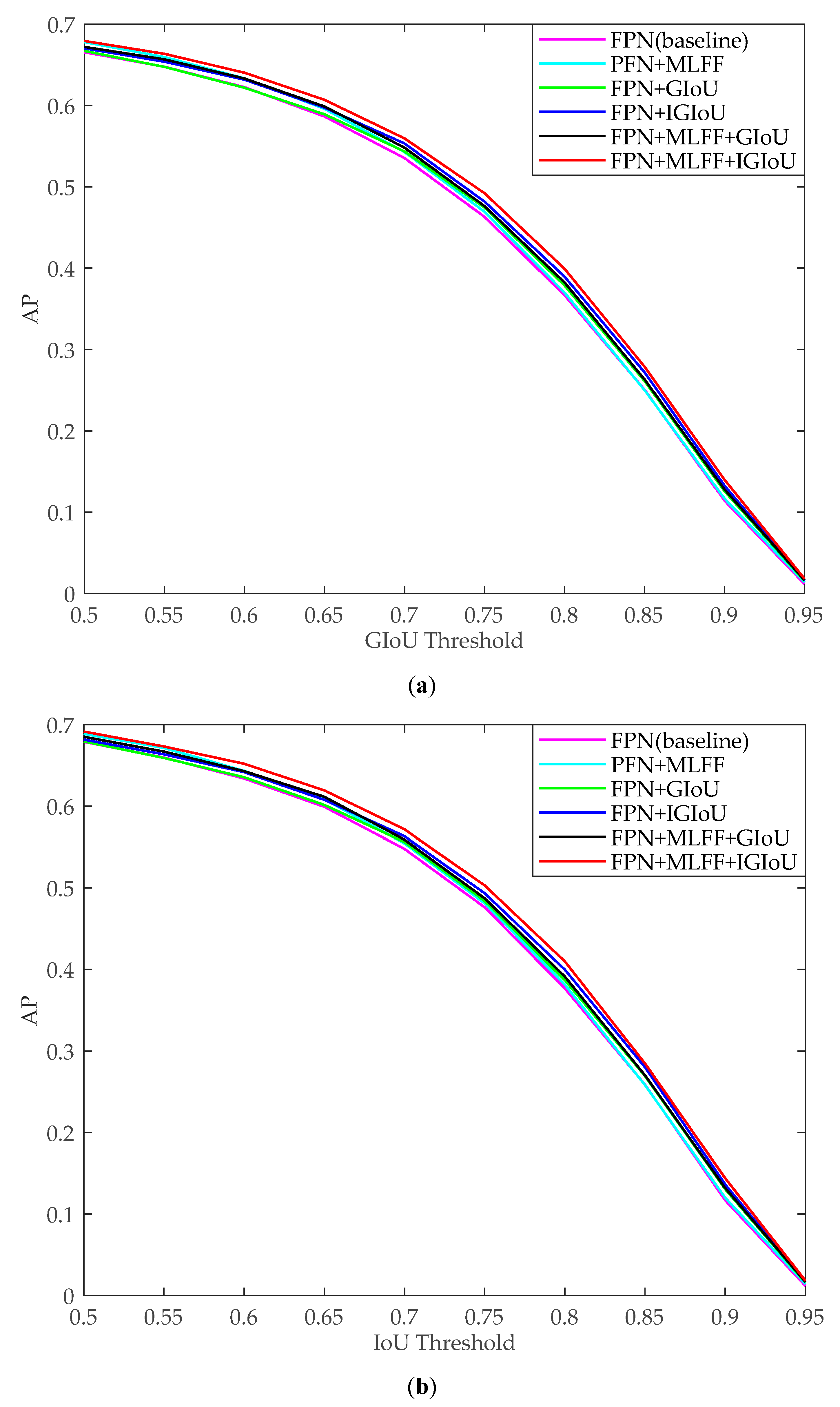
3.1.1. Evaluation of Proposed IGIoU Loss and MLFF Module

To validate the effectiveness of proposed IGIoU loss and MLFF module, the quantitative comparisons between our method and five other methods on NWPU VHR-10 dataset are listed in Table 1. As mentioned in Section 2.2.2, both GIoU and IoU based metrics were used for more comprehensive evaluation.

The Table 1 shows that the FPN+MLFF is superior to FPN in six evaluation metrics, which demonstrates the effectiveness of the MLFF module. The comparisons between FPN+IGIoU and FPN, as well as FPN+IGIoU and FPN+GIoU show that the IGIoU loss is better than the existing smooth L1 loss and GIoU loss. The performance of FPN+MLFF+IGIoU is better than that of FPN+IGIoU and FPN+MLFF, which indicates that the combination of the MLFF module and IGIoU loss is effective. A similar conclusion also applies to MLFF module and GIoU loss. A comparison between FPN+MLFF+IGIoU and FPN+MLFF+GIoU demonstrates that the final combination of an MLFF module and IGIoU loss is superior to the combination of an MLFF module and GIoU loss. In essence, the overall performance of proposed method (FPN+MLFF+IGIoU) on NWPU VHR-10 dataset is the best among the six methods examined, and effectiveness of the MLFF module, IGIoU loss, and their combination are also validated.

To further evaluate our method, the curves of AP with different GIoU (IoU) thresholds of all the comparison methods are shown in Figure 6. Obviously, regardless of the GIoU threshold or IoU threshold, the curves of FPN+MLFF+IGIoU are better than for the other five methods, especially in the range of the 0.65 to 0.8 of GIoU (IoU) threshold. In a word, the effectiveness of the proposed method can be validated for various thresholds, and its superiority is more obvious when the threshold is relatively high.

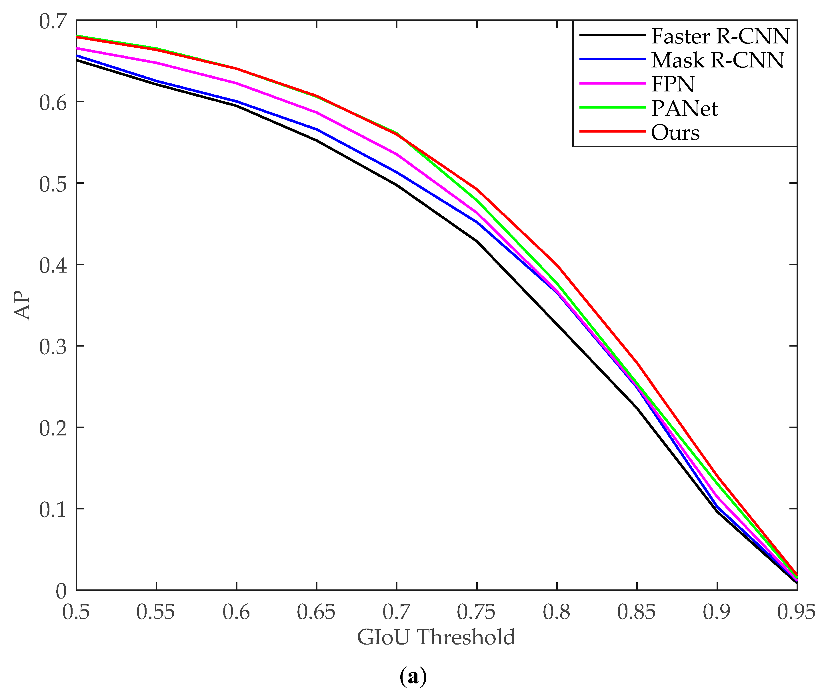
3.1.2. Comparison with the State-of-the-Art Methods

To further validate the overall performance of the proposed method, four state-of-the-art methods were compared wth the proposed method on NWPU VHR-10 dataset, as shown in Table 2. Similar to in Section 3.1.1, both GIoU and IoU were adopted as the metrics.

The Table 2 demonstrates that the proposed method can obtain an absolute gain of 1.7% and 1.4% in terms of GIoU mAP and IoU mAP, respectively, which validates the overall performance of the proposed method. Note that the advantage of the proposed method in terms of AP75 is more obvious, which demonstrates that the proposed method can improve the precision of object localization, the details of which can be seen in Section 4.

Similar to in Section 3.1.1, the curves of AP with different GIoU (IoU) thresholds of all the comparison methods are shown in Figure 7. It can be seen that the proposed method is superior to the state-of-the-art methods, especially when the threshold is in the range of 0.65–0.85, which coincides with the analysis of the previous paragraph.

3.2. Evaluation on DIOR Dataset

3.2.1. Evaluation of Proposed IGIoU Loss and MLFF Module

The quantitative comparisons completed in Section 3.1.1 were also implemented on the DIOR dataset, as shown in Table 3 and Figure 8. Apparently, similar conclusions can be obtained by comparing Table 3 with Table 1. The only difference is that the advantage of the proposed method over the baseline method using the DIOR dataset is not as obvious as the advantage over the NWPU VHR-10 dataset. This may be because the DIOR dataset is larger than the NWPU VHR-10 dataset and its testing images are more challenging to use.

As illustrated in Figure 8, regardless of the GIoU threshold or IoU threshold, the curves of FPN+MLFF+IGIoU are better than for the other five methods, especially in the range of 0.6 to 0.8 of the GIoU (IoU) threshold. Moreover, it can be found that the AP value of our method on the DIOR dataset at different thresholds is more balanced than the AP value on NWPU VHR-10 dataset by comparing Figure 8 with Figure 6. Consequently, the superiority of the proposed method is further validated by considering the challenges and size of the DIOR dataset.

3.2.2. Comparison with the State-of-the-Art Methods

Comparisons similar to Section 3.1.2 were also implemented on the DIOR dataset, as shown in Table 4 and Figure 9, and similar conclusions can be obtained by comparing Table 4 with Table 2. The only difference is that the advantage of the proposed method over the state-of-the-art methods on the DIOR dataset is not as obvious as the advantage on the NWPU VHR-10 dataset. The reason behind this was analyzed in Section 3.2.1.

As shown in Figure 9, the overall performance of the proposed method is superior to the four state-of-the-art methods, especially when the threshold is in the range of 0.7–0.9. The reason for this can also be seen in Section 4.

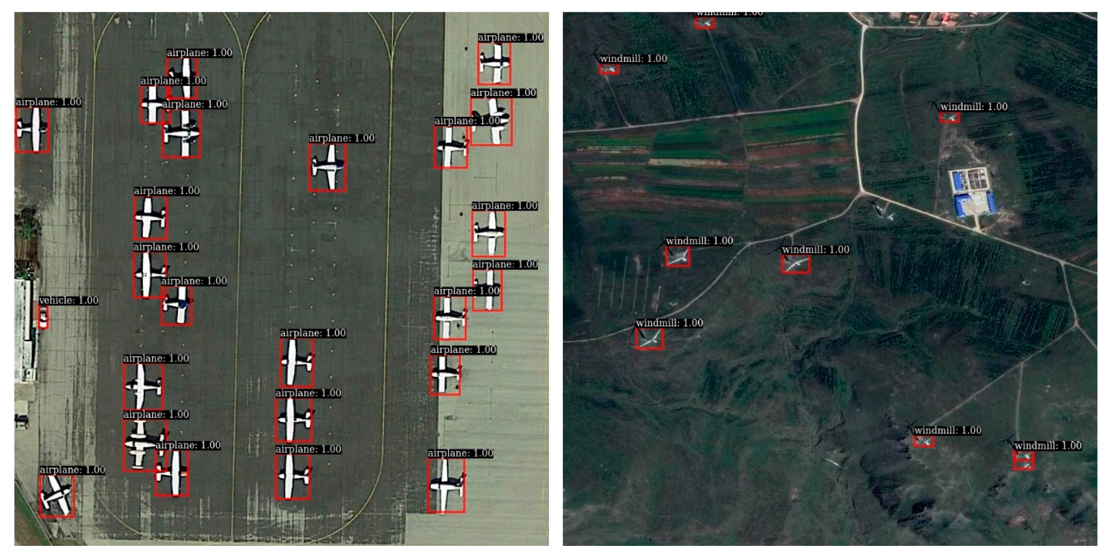
3.3. Subjective Evaluation

To intuitively demonstrate the performance of our method, the detection results of our method on DIOR dataset are visualized. As shown in Figure 10, the detected objects are enclosed by the red bounding box. The classes of detected objects and the corresponding probabilities are also attached to the bounding boxes. Figure 10 demonstrates that our method has an excellent performance on different classes regardless of the scales and orientations of the objects.

4. Discussion

As shown in Table 1 and Table 3, although the proposed method has the best performance in terms of mAP, AP50, and AP75 based on GIoU (IoU), the advantage of the proposed method over other methods is different in three evaluation metrics. Specifically, the advantage of the proposed method is the most obvious in terms of AP75, followed by mAP, and finally by AP50. In other words, the advantage is the most obvious when the threshold of GIoU (IoU) is relatively high. As a matter of fact, the above observations are in accordance with evaluations in terms of curves of AP with different GIoU (IoU) thresholds. As shown in Figure 8 (evaluations on DIOR dataset), the advantage of the proposed method is obvious when the GIoU (IoU) threshold is in the range of 0.6–0.8. In addition, the performance of the proposed method only has a slight improvement when the GIoU (IoU) threshold is in the range of 0.5–0.6 or 0.8–0.95. Similar observations can also be obtained from Figure 6 (evaluations on the NWPU VHR-10 dataset).

The major contributions of this paper focus on the improvement of bounding box regression, which will improve the precision of object localization. Therefore, the advantage of the proposed method over other methods is obvious when the metric of object localization is relatively strict (e.g., the IoU or GIoU threshold is in the range of 0.6–0.8 for the DIOR dataset). However, the advantage no longer exists if the metric is loose or too strict (e.g., the IoU or GIoU threshold is in the range of 0.5–0.6 or 0.8–0.95 for the DIOR dataset).

5. Conclusions

A novel ODRSIs method based on improved bounding box regression and multi-level features fusion was proposed in this paper. First, a new metric named GIoU, which considers both cases of overlapping and non-overlapping between two bounding boxes, was employed to tackle the problem that IoU can not measure the distance in the case of nonoverlapping between two bounding boxes. Second, a novel bounding box regression loss named IGIoU loss was proposed, which can not only optimize metrics (i.e., GIoU) directly but also overcomes the problem that existing GIoU based bounding box regression loss cannot adaptively change the gradient based on the GIoU value. Finally, to handle the problem that the feature extraction scheme of region proposals of the existing method cannot make full use of multi-level features, an MLFF module was proposed and incorporated into the existing hierarchical deep network. The quantitative evaluations on the DIOR and NWPU VHR-10 datasets demonstrate the effectiveness of the proposed method. Specifically, incorporating MLFF, IGIoU loss, and their combination into the baseline method separately achieves absolute gains of 0.7%, 1.4%, and 2.2% or so in terms of COCO mAP on the DIOR dataset, and achieves an absolute gain of 1.0%, 2.0%, and 2.7% on the NWPU VHR-10 dataset, respectively. Moreover, the evaluations in terms of the curves of AP with different thresholds demonstrate that the advantage of the proposed method over other methods is obvious when the threshold is relatively high (e.g., IoU or GIoU threshold is in the range of 0.6–0.8 for the DIOR dataset), which indicates that the proposed method can improve the precision of object localization. Moreover, the comparison between four state-of-the-art methods and the proposed method demonstates that the overall performance of the proposed method has achieved a state-of-the-art level performance.

The GIoU employed in this paper can be applied to other methods in ODRSIs, and the proposed IGIoU loss can also be used as the alternative to existing bounding box regression loss in other object detection methods. Moreover, the proposed MLFF module can be easily embedded into the two-stage object detection methods where the backbone is a hierarchical deep network. Our future works involve extending the proposed method to detect the objects with oriented bounding boxes proposed by Xia et al. [51] and Ding et. al. [52], as well as conducting evaluations on the DOTA dataset.

References

1. Liao, W.; Vancoillie, F.; Gao, L.; Li, L.; Zhang, B.; Chanussot, J. Deep learning for fusion of APEX hyperspectral and full-waveform LiDAR remote sensing data for tree species mapping. IEEE Access 2018, 6, 68716–68729. [Google Scholar] [CrossRef]
2. Zhang, L.; Zhang, J.; Wei, W.; Zhang, Y. Learning Discriminative Compact Representation for Hyperspectral Imagery Classification. IEEE Trans. Geosci. Remote Sens. 2019, 57, 8276–8289. [Google Scholar] [CrossRef]
3. Lv, X.; Ming, D.; Lu, T.; Zhou, K.; Wang, M.; Bao, H. A new method for region-based majority voting CNNs for very high resolution image classification. Remote Sens. 2018, 10, 1946. [Google Scholar] [CrossRef] [Green Version]
4. Lv, X.; Ming, D.; Chen, Y.; Wang, M. Very high resolution remote sensing image classification with SEEDS-CNN and scale effect analysis for superpixel CNN classification. Int. J. Remote Sens. 2019, 40, 506–531. [Google Scholar] [CrossRef]
5. Han, J.; Zhang, D.; Cheng, G.; Liu, N.; Xu, D. Advanced Deep-Learning Techniques for Salient and Category-Specific Object Detection: A Survey. IEEE Signal Process Mag. 2018, 35, 84–100. [Google Scholar] [CrossRef]
6. Cheng, G.; Han, J.; Zhou, P.; Xu, D. Learning Rotation-Invariant and Fisher Discriminative Convolutional Neural Networks for Object Detection. IEEE Trans. Image Process. 2019, 28, 265–278. [Google Scholar] [CrossRef]
7. Zhang, L.; Zhang, Y.; Yan, H.; Gao, Y.; Wei, W. Salient object detection in hyperspectral imagery using multi-scale spectral-spatial gradient. Neurocomputing 2018, 291, 215–225. [Google Scholar] [CrossRef]
8. Liao, W.; Bellens, R.; Pizurica, A.; Philips, W.; Pi, Y. Classification of hyperspectral data over urban areas using directional morphological profiles and semi-supervised feature extraction. IEEE J. Sel. Top. Appl. Earth Obs. Remote Sens. 2012, 5, 1177–1190. [Google Scholar] [CrossRef]
9. Gao, L.; Zhao, B.; Jia, X.; Liao, W.; Zhang, B. Optimized Kernel Minimum Noise Fraction Transformation for Hyperspectral Image Classification. Remote Sens. 2017, 9, 548. [Google Scholar] [CrossRef] [Green Version]
10. Du, L.; You, X.; Li, K.; Meng, L.; Cheng, G.; Xiong, L.; Wang, G. Multi-modal deep learning for landform recognition. ISPRS J. Photogramm. Remote Sens. 2019, 158, 63–75. [Google Scholar] [CrossRef]
11. Zhang, L.; Shi, Z.; Wu, J. A hierarchical oil tank detector with deep surrounding features for high-resolution optical satellite imagery. IEEE J. Sel. Top. Appl. Earth Obs. Remote Sens. 2015, 8, 4895–4909. [Google Scholar] [CrossRef]
12. Stankov, K.; He, D. Detection of buildings in multispectral very high spatial resolution images using the percentage occupancy hit-or-miss transform. IEEE J. Sel. Top. Appl. Earth Obs. Remote Sens. 2014, 7, 4069–4080. [Google Scholar] [CrossRef]
13. Han, X.; Zhong, Y.; Zhang, L. An Efficient and Robust Integrated Geospatial Object Detection Framework for High Spatial Resolution Remote Sensing Imagery. Remote Sens. 2017, 9, 666. [Google Scholar] [CrossRef] [Green Version]
14. Lowe, D. Distinctive image features from scale-invariant keypoints. Int. J. Comput. Vis. 2004, 60, 91–110. [Google Scholar] [CrossRef]
15. Li, F.; Perona, P. A bayesian hierarchical model for learning natural scene categories. In Proceedings of the IEEE Conference on Computer Vision and Pattern Recognition, San Diego, CA, USA, 21–23 September 2005; pp. 524–531. [Google Scholar]
16. Dalal, N.; Triggs, B. Histograms of oriented gradients for human detection. In Proceedings of the IEEE Conference on Computer Vision and Pattern Recognition, San Diego, CA, USA, 21–23 September 2005; pp. 886–893. [Google Scholar]
17. Felzenszwalb, P.; Girshick, R.; McAllester, D.; Ramanan, D. Object detection with discriminatively trained part-based models. IEEE Trans. Pattern Anal. Mach. Intell. 2009, 32, 1627–1645. [Google Scholar] [CrossRef] [PubMed] [Green Version]
18. Sun, H.; Sun, X.; Wang, H.; Li, Y.; Li, X. Automatic target detection in high-resolution remote sensing images using spatial sparse coding bag-of-words model. IEEE Geosci. Remote Sens. Lett. 2011, 9, 109–113. [Google Scholar] [CrossRef]
19. Hyvärinen, A.; Oja, E. Independent component analysis: Algorithms and applications. Neural Netw. 2000, 13, 411–430. [Google Scholar] [CrossRef] [Green Version]
20. Zhang, D.; Meng, D.; Han, J. Co-saliency detection via a self-paced multiple-instance learning framework. IEEE Trans. Pattern Anal. Mach. Intell. 2016, 39, 865–878. [Google Scholar] [CrossRef]
21. Han, J.; Zhang, D.; Hu, X.; Guo, L.; Ren, J.; Wu, F. Background prior-based salient object detection via deep reconstruction residual. IEEE Trans. Circuits Syst. Video Technol. 2014, 25, 1309–1321. [Google Scholar]
22. Han, J.; Yao, X.; Cheng, G.; Feng, X.; Xu, D. P-CNN: Part-Based Convolutional Neural Networks for Fine-Grained Visual Categorization. IEEE Trans. Pattern Anal. Mach. Intell. 2019. [Google Scholar] [CrossRef]
23. Han, J.; Ji, X.; Hu, X.; Zhu, D.; Li, K.; Jiang, X.; Cui, G.; Guo, L.; Liu, T. Representing and retrieving video shots in human-centric brain imaging space. IEEE Trans. Image Process 2013, 22, 2723–2736. [Google Scholar] [PubMed]
24. Redmon, J.; Divvala, S.; Girshick, R.; Farhadi, A. You only look once: Unified, real-time object detection. In Proceedings of the IEEE Conference on Computer Vision and Pattern Recognition, Victoria, BC, Canada, 1–3 June 2016; pp. 779–788. [Google Scholar]
25. Redmon, J.; Farhadi, A. YOLO9000: Better, faster, stronger. In Proceedings of the IEEE Conference on Computer Vision and Pattern Recognition, Honolulu, HI, USA, 21–26 June 2017; pp. 7263–7271. [Google Scholar]
26. Redmon, J.; Farhadi, A. Yolov3: An incremental improvement. arXiv 2018, arXiv:1804.02767. [Google Scholar]
27. Liu, W.; Anguelov, D.; Erhan, D.; Szegedy, C.; Reed, S.; Fu, C.; Berg, A. SSD: Single Shot MultiBox Detector. In Proceedings of the European Conference on Computer Vision, Las Vegas, NV, USA, 27–30 June 2016; pp. 21–37. [Google Scholar]
28. Liu, W.; Ma, L.; Wang, J. Detection of Multiclass Objects in Optical Remote Sensing Images. IEEE Geosci. Remote Sens. Lett. 2018, 16, 791–795. [Google Scholar] [CrossRef]
29. Chen, S.; Zhan, R.; Zhang, J. Geospatial object detection in remote sensing imagery based on multiscale single-shot detector with activated semantics. Remote Sens. 2018, 10, 820. [Google Scholar] [CrossRef] [Green Version]
30. Tang, T.; Zhou, S.; Deng, Z.; Lei, L.; Zou, H. Arbitrary-oriented vehicle detection in aerial imagery with single convolutional neural networks. Remote Sens. 2017, 9, 1170. [Google Scholar] [CrossRef] [Green Version]
31. Tayara, H.; Chong, K. Object detection in very high-resolution aerial images using one-stage densely connected feature pyramid network. Sensors 2018, 18, 3341. [Google Scholar] [CrossRef] [Green Version]
32. Chen, Z.; Zhang, T.; Ouyang, C. End-to-end airplane detection using transfer learning in remote sensing images. Remote Sens. 2018, 10, 139. [Google Scholar] [CrossRef] [Green Version]
33. Ren, S.; He, K.; Girshick, R.; Sun, J. Faster R-CNN: Towards real-time object detection with region proposal networks. In Proceedings of the Advances in Neural Information Processing Systems, Montreal, QC, Canada, 7–12 December 2015; pp. 91–99. [Google Scholar]
34. Dai, J.; Li, Y.; He, K.; Sun, J. R-fcn: Object detection via region-based fully convolutional networks. In Proceedings of the Advances in Neural Information Processing Systems, Barcelona, Spain, 5–10 December 2016; pp. 379–387. [Google Scholar]
35. Lin, T.; Dollár, P.; Girshick, R.; He, K.; Hariharan, B.; Belongie, S. Feature pyramid networks for object detection. In Proceedings of the IEEE Conference on Computer Vision and Pattern Recognition, Honolulu, HI, USA, 21–26 June 2017; pp. 2117–2125. [Google Scholar]
36. Li, K.; Cheng, G.; Bu, S.; You, X. Rotation-insensitive and context-augmented object detection in remote sensing images. IEEE Trans. Geosci. Remote Sens. 2017, 56, 2337–2348. [Google Scholar] [CrossRef]
37. Zhong, Y.; Han, X.; Zhang, L. Multi-class geospatial object detection based on a position-sensitive balancing framework for high spatial resolution remote sensing imagery. ISPRS J. Photogramm. Remote Sens. 2018, 138, 281–294. [Google Scholar] [CrossRef]
38. Chen, C.; Gong, W.; Chen, Y.; Li, W. Object Detection in Remote Sensing Images Based on a Scene-Contextual Feature Pyramid Network. Remote Sens. 2019, 11, 339. [Google Scholar] [CrossRef] [Green Version]
39. Xie, S.; Girshick, R.; Dollár, P.; Tu, Z.; He, K. Aggregated residual transformations for deep neural networks. In Proceedings of the IEEE Conference on Computer Vision and Pattern Recognition, Honolulu, HI, USA, 21–26 June 2017; pp. 1492–1500. [Google Scholar]
40. Wu, Y.; He, K. Group normalization. In Proceedings of the European Conference on Computer Vision, Munich, Germany, 8–14 September 2018; pp. 3–19. [Google Scholar]
41. Ioffe, S.; Szegedy, C. Batch normalization: Accelerating deep network training by reducing internal covariate shift. arXiv 2015, arXiv:1502.03167. [Google Scholar]
42. Cheng, G.; Zhou, P.; Han, J. Learning rotation-invariant convolutional neural networks for object detection in VHR optical remote sensing images. IEEE Trans. Geosci. Remote Sens. 2016, 54, 7405–7415. [Google Scholar] [CrossRef]
43. Rezatofighi, H.; Tsoi, N.; Gwak, J.; Sadeghian, A.; Reid, I.; Savarese, S. Generalized intersection over union: A metric and a loss for bounding box regression. In Proceedings of the IEEE Conference on Computer Vision and Pattern Recognition, Long Beach, CA, USA, 16–20 June 2019; pp. 658–666. [Google Scholar]
44. He, K.; Gkioxari, G.; Dollár, P.; Girshick, R. Mask r-cnn. In Proceedings of the IEEE Conference on Computer Vision and Pattern Recognition, Honolulu, HI, USA, 21–26 June 2017; pp. 2961–2969. [Google Scholar]
45. Cheng, G.; Han, J.; Zhou, P.; Guo, L. Multi-class geospatial object detection and geographic image classification based on collection of part detectors. ISPRS J. Photogramm. Remote Sens. 2014, 98, 119–132. [Google Scholar] [CrossRef]
46. Cheng, G.; Han, J. A survey on object detection in optical remote sensing images. ISPRS J. Photogramm. Remote Sens. 2016, 117, 11–28. [Google Scholar] [CrossRef] [Green Version]
47. Cramer, M. The DGPF-test on digital airborne camera evaluation–overview and test design. Photogramm. Fernerkund. Geoinf. 2010, 2010, 73–82. [Google Scholar] [CrossRef] [PubMed]
48. Yao, X.; Han, J.; Cheng, G.; Qian, X.; Guo, L. Semantic Annotation of High-Resolution Satellite Images via Weakly Supervised Learning. IEEE Trans. Geosci. Remote Sens. 2016, 54, 3660–3671. [Google Scholar] [CrossRef]
49. Morsier, F.; Tuia, D.; Borgeaud, M.; Gass, V.; Thiran, J. Semi-Supervised Novelty Detection Using SVM Entire Solution Path. IEEE Trans. Geosci. Remote Sens. 2013, 51, 1939–1950. [Google Scholar] [CrossRef]
50. Li, K.; Wan, G.; Cheng, G.; Meng, L.; Han, J. Object Detection in Optical Remote Sensing Images: A Survey and A New Benchmark. ISPRS J. Photogramm. Remote Sens. 2020, 159, 296–307. [Google Scholar] [CrossRef]
51. Xia, G.; Bai, X.; Ding, J.; Zhu, Z.; Belongie, S.; Luo, J.; Datcu, M.; Pelillo, M.; Zhang, L. DOTA: A large-scale dataset for object detection in aerial images. In Proceedings of the IEEE Conference on Computer Vision and Pattern Recognition, Salt Lake City, UT, USA, 18–22 June 2018; pp. 3974–3983. [Google Scholar]
52. Ding, J.; Xue, N.; Long, Y.; Xia, G.; Lu, Q. Learning RoI Transformer for Oriented Object Detection in Aerial Images. In Proceedings of the IEEE Conference on Computer Vision and Pattern Recognition, Long Beach, CA, USA, 16–20 June 2019; pp. 2849–2858. [Google Scholar]
53. Lin, T.; Maire, M.; Belongie, S.; Hays, J.; Perona, P.; Ramanan, D.; Dollár, P.; Zitnick, C. Microsoft coco: Common objects in context. In Proceedings of the European Conference on Computer Vision, Zurich, Switzerland, 6–12 September 2014; pp. 740–755. [Google Scholar]
54. Yang, X.; Sun, H.; Fu, K.; Yang, J.; Sun, X.; Yan, M.; Guo, Z. Automatic ship detection in remote sensing images from google earth of complex scenes based on multiscale rotation dense feature pyramid networks. Remote Sens. 2018, 10, 132. [Google Scholar] [CrossRef] [Green Version]
55. Guo, W.; Yang, W.; Zhang, H.; Hua, G. Geospatial object detection in high resolution satellite images based on multi-scale convolutional neural network. Remote Sens. 2018, 10, 131. [Google Scholar] [CrossRef] [Green Version]
56. Deng, Z.; Sun, H.; Zhou, S.; Zhao, J.; Lei, L.; Zou, H. Multi-scale object detection in remote sensing imagery with convolutional neural networks. ISPRS J. Photogramm. Remote Sens. 2018, 145, 3–22. [Google Scholar] [CrossRef]
57. Everingham, M.; Vangool, L.; Williams, C.; Winn, J.; Zisserman, A. The Pascal Visual Object Classes (VOC) Challenge. Int. J. Comput. Vis. 2010, 88, 303–338. [Google Scholar] [CrossRef] [Green Version]
58. Rumelhart, D.; Hinton, G.; Williams, R. Learning representations by back-propagating errors. Nature 1988, 323, 696–699. [Google Scholar] [CrossRef]
59. Liu, S.; Qi, L.; Qin, H.; Shi, J.; Jia, J. Path aggregation network for instance segmentation. In Proceedings of the IEEE Conference on Computer Vision and Pattern Recognition, Salt Lake City, UT, USA, 18–22 June 2018; pp. 8759–8768. [Google Scholar]
Figure 1. Framework of our object detection in remote sensing images (ODRSIs) method. (a) feature pyramid network (FPN) backbone; (b) Multi-level features fusion; (c) Classification and bounding box regression based on IGIoU loss.
Remotesensing 12 00143 g001
Figure 2. Illustration of two intersecting (non-overlapping) bounding boxes. (a) Two intersecting bounding boxes; (b) Two non-overlapping bounding boxes. The rectangles enclosed by a green solid line, red solid line, and blue dashed line separately denote the ground truth box B G T , predicted bounding box B P T , and smallest enclosing box B E C .
Remotesensing 12 00143 g002
Figure 3. Illustration of GIoU and IGIoU loss.
Remotesensing 12 00143 g003
Figure 4. Total number of object instances of each category in two datasets.
Remotesensing 12 00143 g004
Figure 5. Examples of images from the NWPU VHR-10 and DIOR benchmark dataset, where (a)(j) denotes the categories from the NWPU VHR-10 dataset, and (a)(t) represents the categories from the DIOR dataset.
Remotesensing 12 00143 g005aRemotesensing 12 00143 g005b
Figure 6. Comparison with baseline methods on NWPU VHR-10 dataset in terms of curves of AP with different GIoU (IoU) thresholds. (a) GIoU threshold; (b) IoU threshold.
Remotesensing 12 00143 g006
Figure 7. Comparison with four state-of-the-art methods on NWPU VHR-10 dataset in terms of curves of AP with different GIoU (IoU) thresholds. (a) GIoU threshold; (b) IoU threshold.
Remotesensing 12 00143 g007aRemotesensing 12 00143 g007b
Figure 8. Comparison with baseline methods on the DIOR dataset in terms of curves of AP with different GIoU (IoU) thresholds. (a) GIoU threshold; (b) IoU threshold.
Remotesensing 12 00143 g008
Figure 9. Comparison with four state-of-the-art methods on DIOR dataset in terms of curves of AP with different GIoU (IoU) thresholds. (a) GIoU threshold; (b) IoU threshold.
Remotesensing 12 00143 g009aRemotesensing 12 00143 g009b
Figure 10. Subjective evaluations on 10 testing images from the DIOR dataset.
Remotesensing 12 00143 g010aRemotesensing 12 00143 g010bRemotesensing 12 00143 g010c