SST Anomalies in the Mozambique Channel Using Remote Sensing and Numerical Modeling Data

Abstract

Based on both satellite remote sensing sea surface temperature (SST) data and numerical model results, SST warming differences in the Mozambique Channel (MC) west of the Madagascar Island (MI) were found with respect to the SST east of the MI along the same latitude. The mean SST west of the MI is up to about 3.0 °C warmer than that east of the MI. The SST differences exist all year round and the maximum value appears in October. The area of the highest SST is located in the northern part of the MC. Potential factors causing the SST anomalies could be sea surface wind, heat flux and oceanic flow advection. The presence of the MI results in weakening wind in the MC and in turn causes weakening of the mixing in the upper oceans, thus the surface mixed layer depth becomes shallower. There is more precipitation on the east of the MI than that inside the MC because of the orographic effects. Different precipitation patterns and types of clouds result in different solar radiant heat fluxes across both sides of the MI. Warm water advected from the equatorial area also contribute to the SST warm anomalies.

1. Introduction

The existence of islands has significant impacts on the local hydrological environment, especially influencing the physical processes in the lee of islands [1,2,3,4,5,6,7,8,9,10]. These processes can be categorized into two types: (i) oceanic response to wind wakes; and (ii) variation in oceanic current when it passes an island (hereafter referred to as oceanic current wakes). Realistic island wakes could be very complicated because both types of processes take place simultaneously.

For the first type, when the wind blows across an island, the intensity of the wind behind the island is drastically reduced because the roughness of the island surface is much larger than that of the sea surface and mountains over the island also have a blocking effect. Weakening wind intensity weakens the mixing of the upper oceans and the surface mixed layer depth becomes shallow. The cloud amount in the lee of the island decreases because of the topographic rain effect. Ekman pumping can result in local upwelling or downwelling and even the formation of cyclonic or anticyclonic eddies. For the second type, oceanic current wakes can be differentiated into two types based on their vorticity generation mechanisms [9,10,11]: deep-water and shallow-water island wakes. The difference between shallow-water and deep-water island wakes (with/without the shelf slope) is also explored. There are three possible vorticity sources: (1) lateral stress; (2) bottom stress; and (3) tilting of the baroclinic flow. If the primary vorticity source comes from lateral stress, the island wake is considered a deep-water one; when bottom stress is dominant, the wake is a shallow-water wake, where the horizontal vorticity can be tilted into the vertical component through baroclinic processes. Therefore, the physical parameters can be dramatically altered with the two types of island effects on the lee side of an island, such as sea surface temperature (SST).

The abnormal warm SST resulting from the presence of an island has been found in different oceanic areas [4,12,13,14,15,16]. Barton et al. [4] found that the mountainous Canary Islands present obstacles to the trade winds and to the Canary Current flowing equatorward past them. Barton et al. [12] examined the air–sea interactions in the Canary Islands region using Synthetic Aperture Radar (SAR) and Advanced Very High Resolution Radiometer (AVHRR) images. They found that the region of weaker wind coincides with a warm “wake”. Xie et al. [13] explored the wake of the Hawaiian island caused by the northeasterly trade. When the broad steady northeasterly trades impinge on Hawaii, wind wakes are formed behind the individual islands and these individual wakes dissipate rather quickly. Caldeira and Marchesiello [14] found a warm water zone on the leeward side of the Atlantic Madeira Island. The warm water zone results from the action of the wind at the expense of a Karman vortex, which makes the area cloudless thus allowing more solar radiation to enter the region. Caldeira et al. [15] analyzed the warm water on the eastern side of Santa Catalina Island, California. The mechanism of the warm water formation in that region is consistent with that of Madeira. Li et al. [16] explored the warm pool southwest of Hainan Island in winter. The seasonal warm pool is due to the small low-level wind speed, which weakens the latent heat release at that level so that the water temperature is higher than in the surrounding waters.

The existence of Madagascar Island (MI) could have significant impacts on the SST on the lee side of the island. The Mozambique Channel (MC) is located southeast of the African continent, between the MI and Mozambique (Figure 1). It is the fourth largest island in the world after Greenland, New Guinea and Kalimantan Island. The channel is about 1600 km long and 386 km wide at its narrowest point. Its depth can reach up to 3292 m. The MI has a sloping, mountainous block of land to the west with the highest elevation measured at 2000 m. The shape of the island is long and narrow, with the northern and southern part being narrower than the middle part. The widest section is 576 km across and its coastline is 3991 km long. The presence of MI has an important influence on the hydrology of the area [17]. It imposes a partitioning of the poleward western boundary flow into two components: one along the western MC (the Mozambique Current) and another along the east coast of Madagascar (the Southeast Madagascar Current).

The present study examined the temporal and spatial variations of the SST anomalies in the MC and investigate potential mechanisms which cause the anomalies. The remainder of this paper is organized as follows. Section 2 describes the data and the numerical model configuration. In Section 3, the spatial and temporal characteristics of the warm SST anomalies are described, and the influences of the wind intensity and heat flux on the SST anomalies are analyzed. Section 4 is the discussion, in which the temperature budget equation is used to analyze the influence of the background oceanic currents. Section 5 is the summary.

2. Data, Model Configuration and Method

2.1. Satellite Data

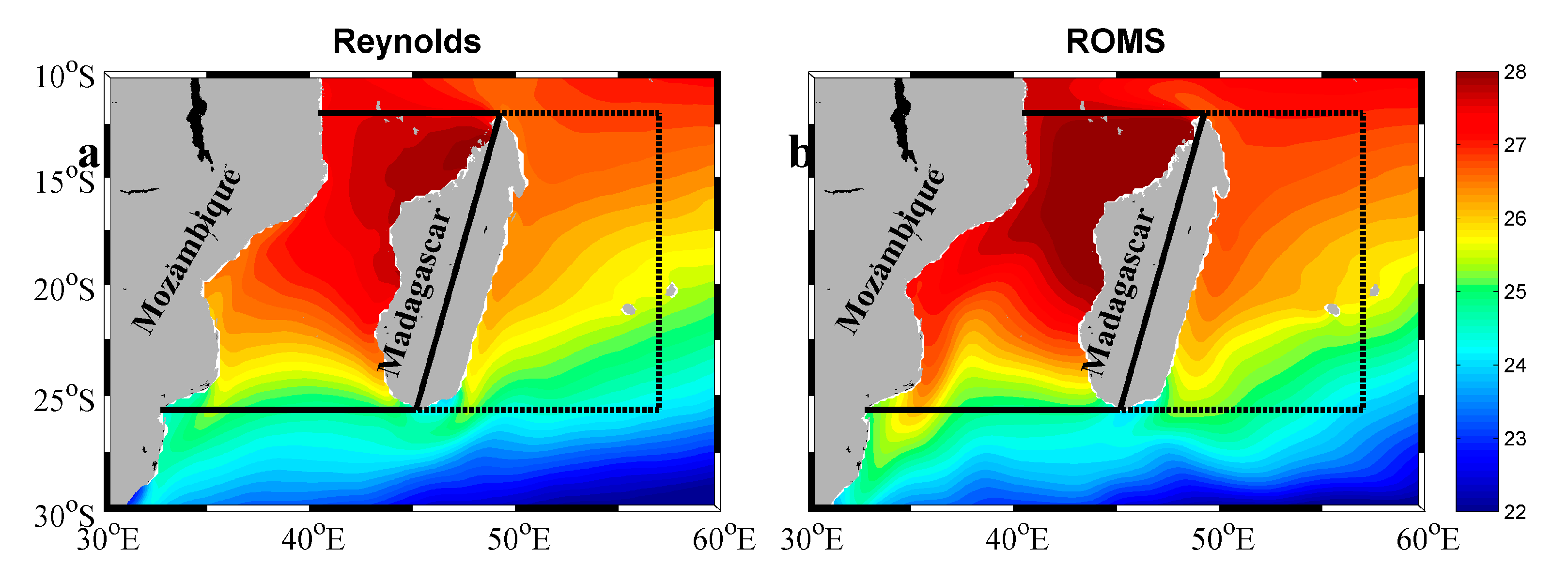
2.1.1. Reynolds’ SST Data

Reynolds’ SST is a series of real-time global analysis products developed by Reynolds et al. [18] (https://www.esrl.noaa.gov/psd/data/gridded/data.noaa.oisst.v2.highres.html). Reynolds’ SST provides global fields that are based on a combination of ocean temperature observations from satellite and in situ platforms (i.e., ships and buoys). Due to their long-term available coverage, the 1992–2014 AVHRR-only monthly averaged data with the spatial resolution of 1/4° were used in this study.

2.1.2. TMI Cloud Data

The Tropical Rainfall Measuring Mission (TRMM) was launched on 27 November 1997, carrying five instruments, including the TRMM Microwave Imager (TMI) [19] (http://www.remss.com/missions/tmi/). The TMI is a multi-channel, dual polarized, conical scanning passive microwave radiometer designed to measure rain rates over a wide swath under the TRMM satellite. The 1998–2014 monthly mean TMI measured cloud liquid water with the spatial resolution of 1/4° × 1/4° was applied to the present study.

2.1.3. AVISO Geostrophic Current Data

The Sea Level Anomalies (SLA) derived geostrophic current data employed in our study were downloaded from the Archiving, Validation, and Interpretation of Satellite Oceanographic (AVISO) data [20] (https://www.aviso.altimetry.fr). The 15-year (January 2000–December 2014) spatial and temporal resolutions are 1/4° × 1/4° and daily, respectively. The AVISO geostrophic current data were used to detect eddies.

2.1.4. AVHRR SST Data

The AVHRR (advanced very high-resolution radiometer) SST data with 1/4° × 1/4° spatial resolution and daily sampling were used in this study. AVHRR is a sensor carried on the NOAA (National Oceanic and Atmospheric Administration) series of meteorological satellites [18] (https://www.noaasis.noaa.gov/NOAASIS/ml/avhrr.html). Since the launch of the TIROS-N satellite in 1979, the AVHRR sensor has continued to perform ground observation missions. The same period of SST anomalies data as that of the AVISO geostrophic current data was used.

2.2. NCEP CFSR Reanalysis Data

The Climate Forecast System Reanalysis (CFSR) data by the National Centers for Environmental Prediction (NCEP) were applied to the present study (https://rda.ucar.edu/). The CFSR global atmosphere resolution is ~38 km with 64 levels. The Regional Ocean Modeling System (ROMS) is driven by 6-hourly surface atmospheric forcings for the period from January 1979 to December 2014, which are from CFSR 93.0 [21] for the first period (from January 1979 to March 2011) and from CFSv2 [22] for the second period (from April 2011 to December 2014). The wind field data near the ground were used to check the influence of the wind speed on the warm SST anomalies. The solar short-wave radiation and long-wave radiation were also used in this study.

2.3. Model Configuration

The model used in this study is the ROMS. The ROMS is a high-resolution, free-surface and topography-following-coordinate oceanic model. It has been widely used in regional ocean simulation, air–sea interaction and ocean dynamics analysis [8,9,10,23,24,25]. The model domain is configured in the region of 30°E–110°E and 30°S–30°N with the 1/8° horizontal grid and 32 vertical levels. The minimum depth at which a higher resolution in the upper layer of the ocean is defined with the parameter hc = 100 m, and the maximum depth is 5000 m. The vertical s-coordinate parameters are 3.0 (surface) and 0.3 (bottom), respectively. The newly defined function of the vertical levels, Vtransform = 2 and Vstretching = 4, were used to select the vertical transform equation and stretching function. The detailed settings of the model can be found in the work of Li et al. [24]. We focused on the area in the Southwest Indian Ocean (30–10°S, 30–60°E) for the period from January 1982 to December 2014. In addition, daily-averaged results of the model output in the year of 2014 were used for further analysis.

2.4. Eddy Automatic Detection.

The eddy detection method used in this study is proposed by Nencioli [26]. Four constraints are defined based on the characteristics of eddy velocity fields:

(1) Along an east–west (EW) section, meridional velocity, v, reverses sign across the eddy center and its magnitude increases away from it.

(2) Along a north–south (NS) section, zonal velocity, u, reverses sign across the eddy center and its magnitude increases away from it: the sense of rotation has to be the same as for v.

(3) Velocity magnitude has a local minimum at the eddy center.

(4) Around the eddy center, the directions of the velocity vectors have to change with a constant sense of rotation, and the directions of two neighboring velocity vectors have to lie within the same or two adjacent quadrants (the four quadrants are defined by the north–south and west–east axes: the first quadrant encompasses all the directions from east to north, the second quadrant encompasses the directions from north to west, the third quadrant encompasses the directions from west to south, and the fourth quadrant encompasses the directions from south to east.

3. Results

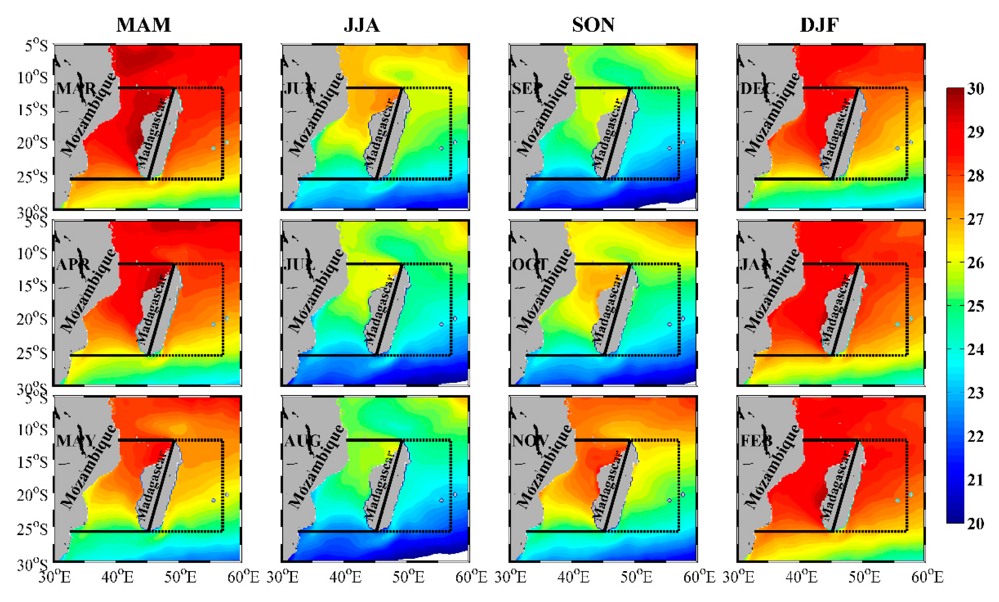
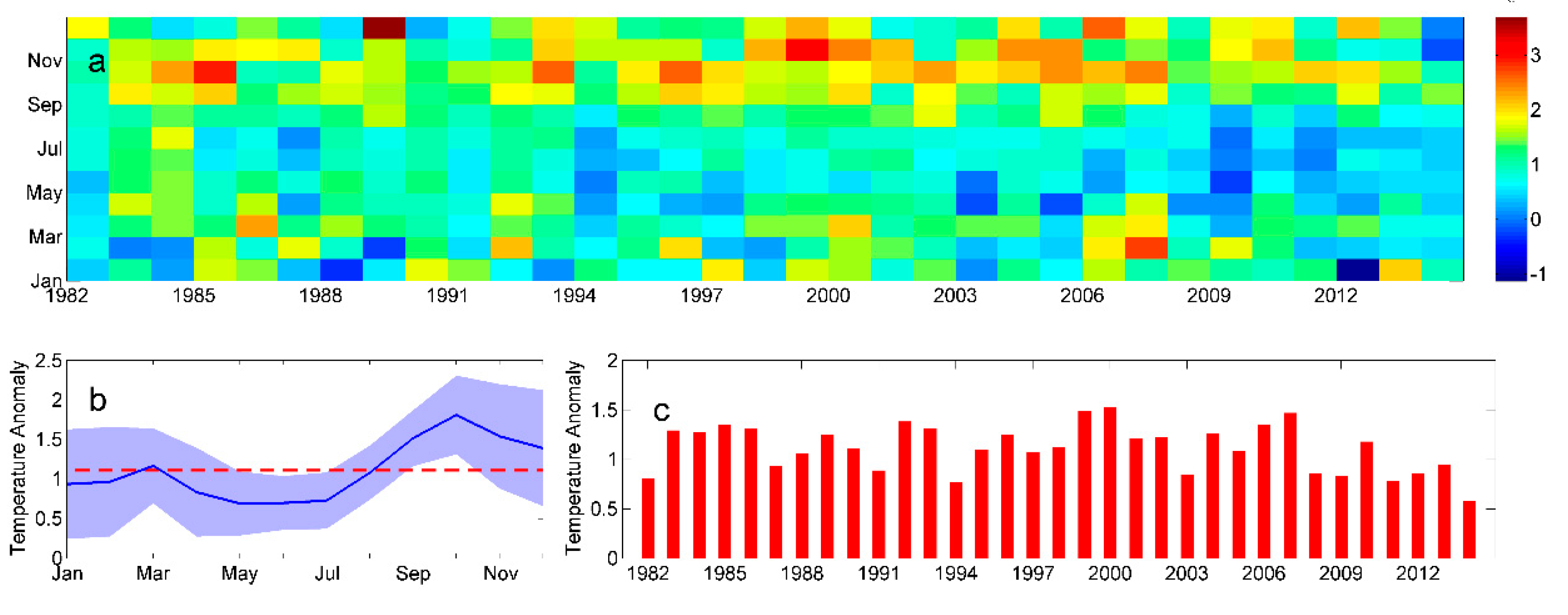
3.1. Phenomena: SST Anomalies in the MC

The study area is divided into two parts: inside the MC (A1-B1-B2-A2, solid line) and east of the MI (B1-C1-C2-B2, dotted line) (Figure 1). The coordinates of the points in Figure 1 are listed in

Table 1. Coordinates of the points forming the sections in Figure 1.

Inside the MC			East of the MI
A1	40°25′E	11°57′S	B1	49°16′E	11°57′S
B1	49°16′E	11°57′S	C1	57°E	11°57′S
A2	32°45′E	25°37′S	B2	45°10′E	25°37′S
B2	45°10′E	25°37′S	C2	57°E	25°37′S

.

The SST averaged over 1982–2014 from the Reynolds’ product and the ROMS results are plotted in Figure 2, which shows that the SST in the study area decreases with increasing latitude. However, the SST in the MC is significantly higher than that on the east of the MI. The highest value of the SST appears on the northwest side of MI. Although the model simulation overestimated the SST when compared to the observation data, the overall SST distribution pattern from the ROMS is similar to that from the observation data. The SST in the MC is about 0.9$°\mathrm{C}$ and 1.2$°\mathrm{C}$ warmer than that on the east of the MI for the Reynolds’ and the ROMS data, respectively. On the east of the MI, the SST contours display a southwest-northeast oriented distribution; inside the channel, the higher SST appears in the northern part. In addition, at the same latitude (~15°S), the SST on the east of the MI is about 26.5$°\mathrm{C}$, which is lower than the SST inside the MC. A cold water tongue spreads into the channel in the southern part inside the channel region.

Monthly modeled SST spatial distributions are plotted in Figure 3, in which the seasonal variation of the SST distribution is clearly presented. The SST in the study area is lower in austral winter (from June to August) and spring (from September to November) than that in summer (from December to February) and fall (from March to May). The highest SST in the channel appears in March. The highest SST on the east of the MI appears in February, which is one month earlier than that inside the MC. The lowest SST occurs in October. Overall, the SST in the Channel is higher than that on the east of the MI all the year round.

To quantify the SST difference between inside the MC and east of the MI, the monthly mean differences of the SST between the inside MC and east of the MI are shown in Figure 4a using the ROMS results from January 1982 to December 2014. The maximum difference value can reach up to 3.7$°\mathrm{C}$ (December 1989). However, in some specific months, the SST in the MC is lower than that on the east of the MI, for example, the value reached −1.2 $°\mathrm{C}$ in January 2012. The temperature anomalies have obvious seasonal variation (Figure 4b). The austral summer values are larger than those in winter. In addition, the standard deviation of the SST difference in the austral summer is much larger than that in winter. The mean value of the SST difference is about 1.2$°\mathrm{C}$. For yearly mean result (Figure 4c), the maximum value appeared in 2000 (1.5 $°\mathrm{C}$), and the minimum value appeared in 2014 (0.7$°\mathrm{C}$).

3.2. Mechanisms: SST Anomalies in the MC

In this section, we try to address the mechanisms which cause the warm SST anomalies in the MC. The potential mechanisms could be the differences in wind-induced mixing, heat flux and advection by oceanic currents between inside the MC and east of the MI.

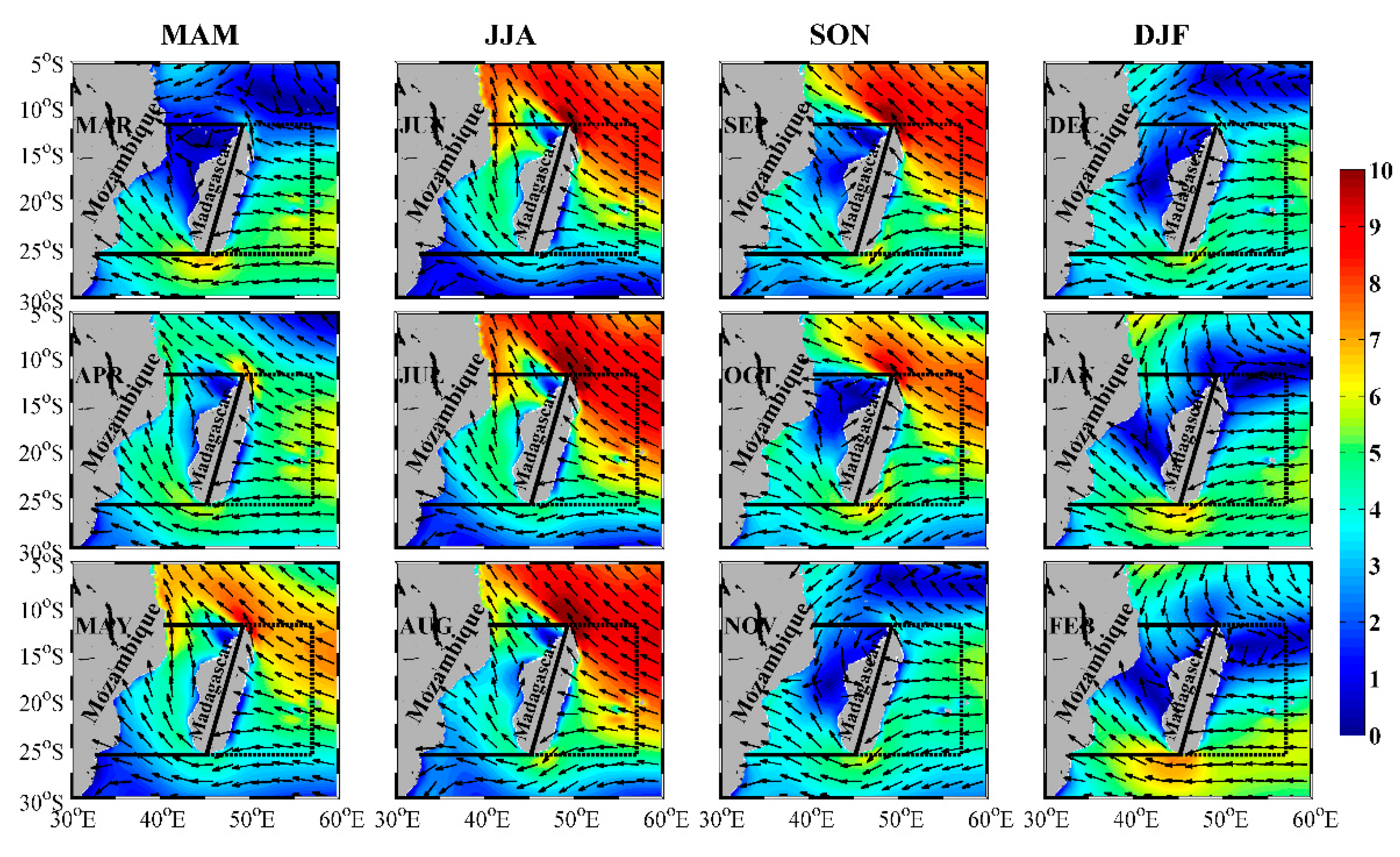
3.2.1. Wind Field Variation

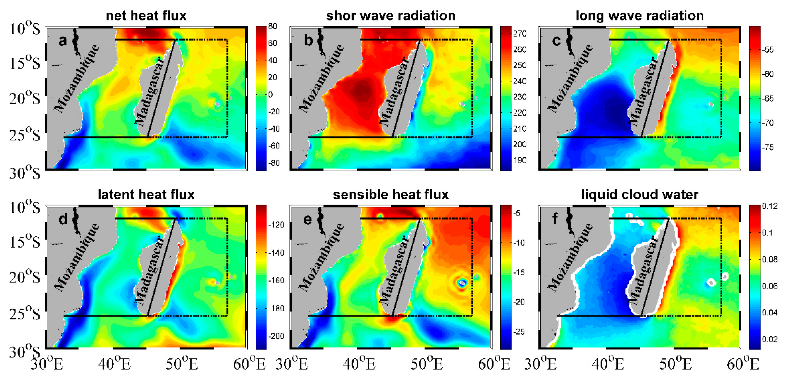
Wind field could affect the SST variation. When the wind blows over the sea surface, sea surface wind stress is generated, and momentum is transferred from the atmosphere to the ocean. Wind stress constitutes the primary driving force of the upper ocean dynamics. The surface wind stress, generated by turbulent mixing effect and shear, strengthens the vertical mixing processes in the surface mixed layer and leads to the deepening of the mixed layer. The stronger is the wind at the sea surface, the more intensive is the mixing in the upper ocean. When the wind passes an island, the intensity of the wind decreases due to both the larger roughness and blockage from the mountains over the island. This phenomenon can be seen clearly in the monthly NCEP CFSR wind field averaged over the period from 1982 to 2014 (Figure 5).

Figure 5 shows that east of the MI is dominated by the easterly wind. When the easterly wind blows through the MI, the intensity of the wind behind the MI is drastically reduced because the roughness of the island surface is much greater than that of the ocean, and the island’s mountains also have a blocking effect. Inside the MC, the smallest wind speed in one year is presented in March. The smallest wind speed (~1 m/s) appears in the north MC. On the east of the MI, the wind speed is about 5 m/s. From March to July, the wind speed in the study area gradually increases. The largest wind speed appears in July. The largest wind speed on the east of the MI is about 9.5 m/s. Inside MC, the largest wind speed is 6.5 m/s, which is smaller than that east of the MI. From July to February, the wind speed in the study area decreases. On the east of the MI, the smallest wind speed in one year is presented in February, which is one month earlier than that inside the MC. Overall, the wind speed in the Channel is smaller than that on the east of the MI all around year.

Comparing the spatial distributions of the monthly SST (Figure 3) with that of the monthly wind field (Figure 5), it was found that the stronger (weaker) winds are associated with lower (higher) SST in terms of spatial and temporal distributions. The reason the SST has high correlation with the wind intensity is that the SST is partially controlled by the surface mixed layer depth, which is strongly affected by the wind intensity. The surface mixed layer depth on the east of the MI is more affected by wind speed than that inside the MC. Since the mixed layer depth is partially controlled by the wind intensity, further analysis on the relationship between the SST and the wind intensity is discussed in Section 3.2.3.

3.2.2. Heat Flux

Net heat flux also has an important effect on the SST variation. The sea surface net heat flux $Q_{net}$ consists of four parts: solar short-wave radiation $Q_{sw}$, outgoing long-wave radiation $Q_{lw}$, latent heat flux $Q_{lat}$, and sensible heat flux $Q_{sen}$:

$$Q_{net}=Q_{sw}+Q_{lw}+Q_{lat}+Q_{sen}$$

(1)

The net heat flux input in the upper ocean plays a direct heating or cooling role on the ocean mixed layer. The positive net heat flux (the ocean gains the heat from the atmosphere) can strengthen the stratification of the mixed layer and weaken vertical mixing, resulting in a shallow mixed layer. On the contrary, when the net heat flux is lost to the atmosphere, it plays a cooling role on the mixed layer. The stratification is weakened, and the turbulent vertical mixing is strengthened, which leads to the deepening of the mixed layer depth. These processes significantly influence the mixed layer and the temperature distribution in the upper ocean.

As stated in Section 2.2, the solar short-wave radiation and outgoing long-wave radiation were from NECP CFSR data directly. The sensible heat flux is given by the standard aerodynamic formula from the ROMS:

$$Q_{sen}={\rho }_a{c}_p{C}_H{V}_{wg}\left(T_a-T_{sfc}\right)$$

(2)

where ${\rho }_a$ is air density, $c_p$ is specific heat of dry air (1004 J·kg⁻¹·K⁻¹), $C_H$ is transfer coefficient for sensible heat (1.75 × 10⁻³), $V_{wg}$ is geostrophic wind speed, and $T_a$ and $T_{sfc}$ represent air temperature and surface temperature of the water, respectively. The latent heat is also given by the standard aerodynamic formula from ROMS:

$$Q_{lat}={\rho }_{a}L{C}_E{V}_{wg}\left(q_{10m}-q_s\right)$$

(3)

where $L$ is latent heat of vaporization (2.5 × 10⁶ J·kg⁻¹), $C_E$ is transfer coefficient for latent heat (1.75 × 10⁻³), and $q_{10m}$ and $q_s$ represent 10-m specific humidity and surface specific humidity, respectively.

Since the heat flux is strongly influenced by the cloud coverage, we discuss the effect of the MI on the cloud coverage before the heat flux distribution is presented. When moist air masses meet with the terrain blocking, the moist air is forced to slowly uplift. The cloud (which could lead to precipitation) thus occurs by adiabatic cooling and condensation [27]. When the wind carrying the moist air is from the east of the MI, it is uplifted over the mountain on the MI, and the cloud is formed. It is expected that higher cloud coverage is presented east of the MI than over the MC (see Figure 6f). The influence of the cloud coverage on the heat flux can be seen on the spatial distribution of the heat flux.

Figure 6 shows the climatology of net heat flux, net long-wave radiation flux, net sensible heat flux, solar short-wave radiation flux, net latent heat flux and liquid cloud water in the study area, which is averaged over 33 years from 1982 to 2014. In Figure 6a, one can see clearly that the net heat flux inside the channel (4.99 Wm⁻²) is larger than that east of the MI (3.87 Wm⁻²). For four components of the net heat flux, it was noticed that the short-wave radiation inside the channel (256.21 Wm⁻²) is much greater than that on the east of the MI (230.77 Wm⁻²) (Figure 6b). The shortwave radiation is related to solar incidence angle and cloud coverage. Since the solar incidence angle is the same on two sides of the MI, there are more clouds east of the MI than that inside the MC (Figure 6f). The magnitude of the outgoing long-wave radiation inside the MC (−70.6 Wm⁻²) is larger than that east of the MI (−62.88 Wm⁻²), which means the ocean inside the MC loses more heat (Figure 6c). The outgoing long-wave radiation is also strongly influenced by the presence of cloud. The magnitude of the sensible heat fluxes inside the MC (−15.58 Wm⁻²) is also larger than that east of the MI (−12.01 Wm⁻²) (Figure 6e). Latent heat of vaporization is the main pathway through which the ocean loses the heat. Li et al. [16] pointed out that a seasonal warm pool resulting from low wind speed and small latent heat loss, appears southwest of Hainan Island in winter. However, in this study area, the latent heat flux inside the channel (−164.87 Wm⁻²) is greater than outside the channel (−151.99 Wm⁻²) (Figure 6d). Since the latent heat flux is affected by both the wind intensity and air humidity (see Equation (3)), the lower and the more latent heat lost to the air when the wind change plays the secondary role in Equation (3).

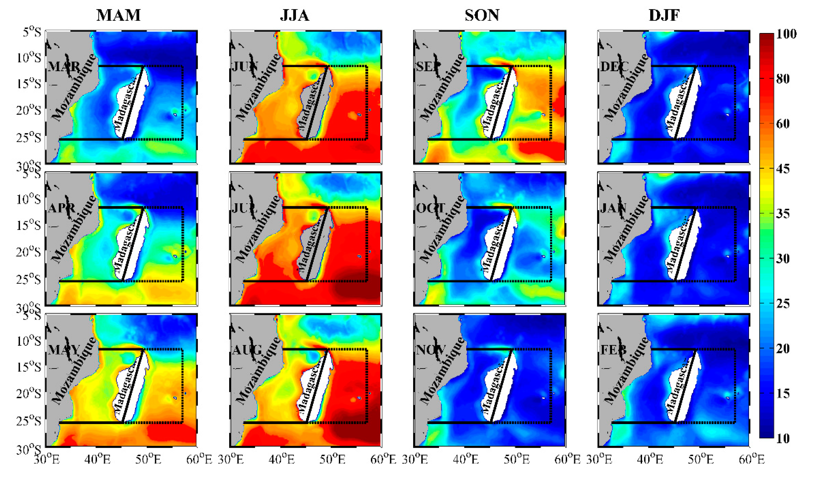
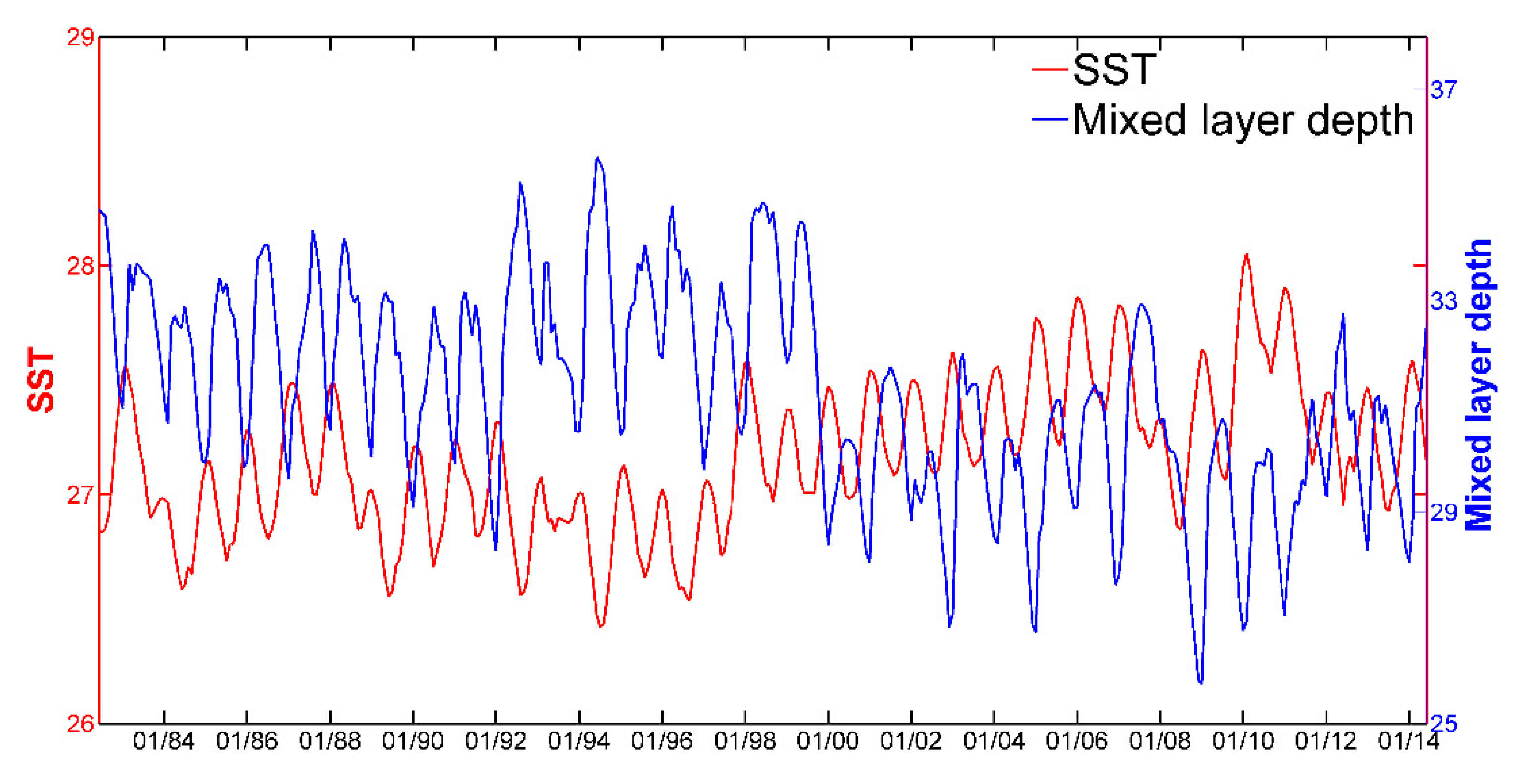
3.2.3. Surface Mixed Layer Depth

The effects of the wind intensity and net heat flux on the SST need to be reflected on the variation of the surface mixed layer depth. The surface mixed layer is a layer in which active turbulence (through sea surface wind and heat flux) homogenizes the stratification to a certain depth by mixing up the subsurface cold water with the surface water (Figure 7).

There are several definitions for the surface mixed layer depth [28]. Typically, a threshold is defined, for which the MLD is the depth at which parameters (potential temperature, potential density or density) changes by a given threshold value relative to one at a near-surface reference depth. In this study, the fixed potential temperature threshold method is used to define the mixed layer depth where the potential temperature decrease by $\Delta T=0.2°\mathrm{C}$, compared to that at the sea surface, where T denotes the potential temperature [29,30].

The monthly surface mixed layer depth averaged over the 33-year ROMS results from 1982 to 2014 is plotted in Figure 8. The surface mixed layer depth carries significant seasonal variations with obvious differences both inside the MC and east of the MI. The deepest surface mixed layer (110 m) appears in the area east of the MI in July when it is in the austral winter. The deepest surface mixed layer (80 m) inside the MC also appears in July, which is shallower than that outside the MC. The shallowest mixed layer (about 10 m) appears in December both inside and outside the MC. In austral summer, the surface mixed layer depth in the study area is the shallowest among all the seasons. Overall, the surface mixed layer depth in the MC is shallower than that east of the MI. There is significant difference of the surface mixed layer depth between inside the MC and east of the MI. The difference reaches the maximum value (18 m) in August.

In summary, in Section 3.2.1, Section 3.2.2 and Section 3.2.3, we discuss the factors affecting the SST: wind intensity, net heat flux and surface mixed layer depth. The wind and net heat flux are external forces for the SST variation, which take effects through changing the surface mixed layer depth, therefore the surface mixed layer depth variation should have the direct correlation with the SST variation, which can be found in the time series of SST and surface mixed layer depth (see Figure 9). The correlation coefficient between the surface layer depth and SST is −0.75.

4. Discussion

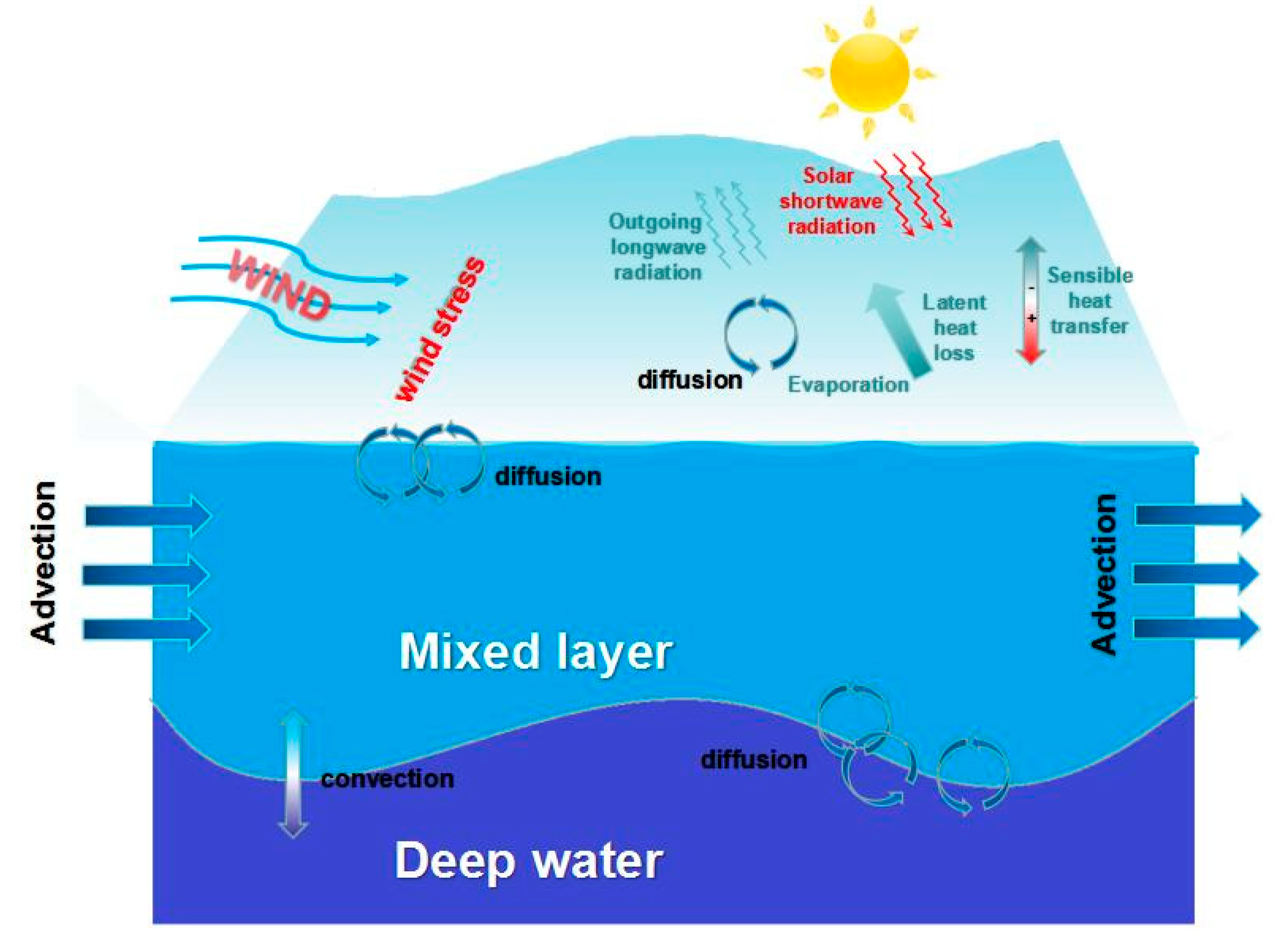
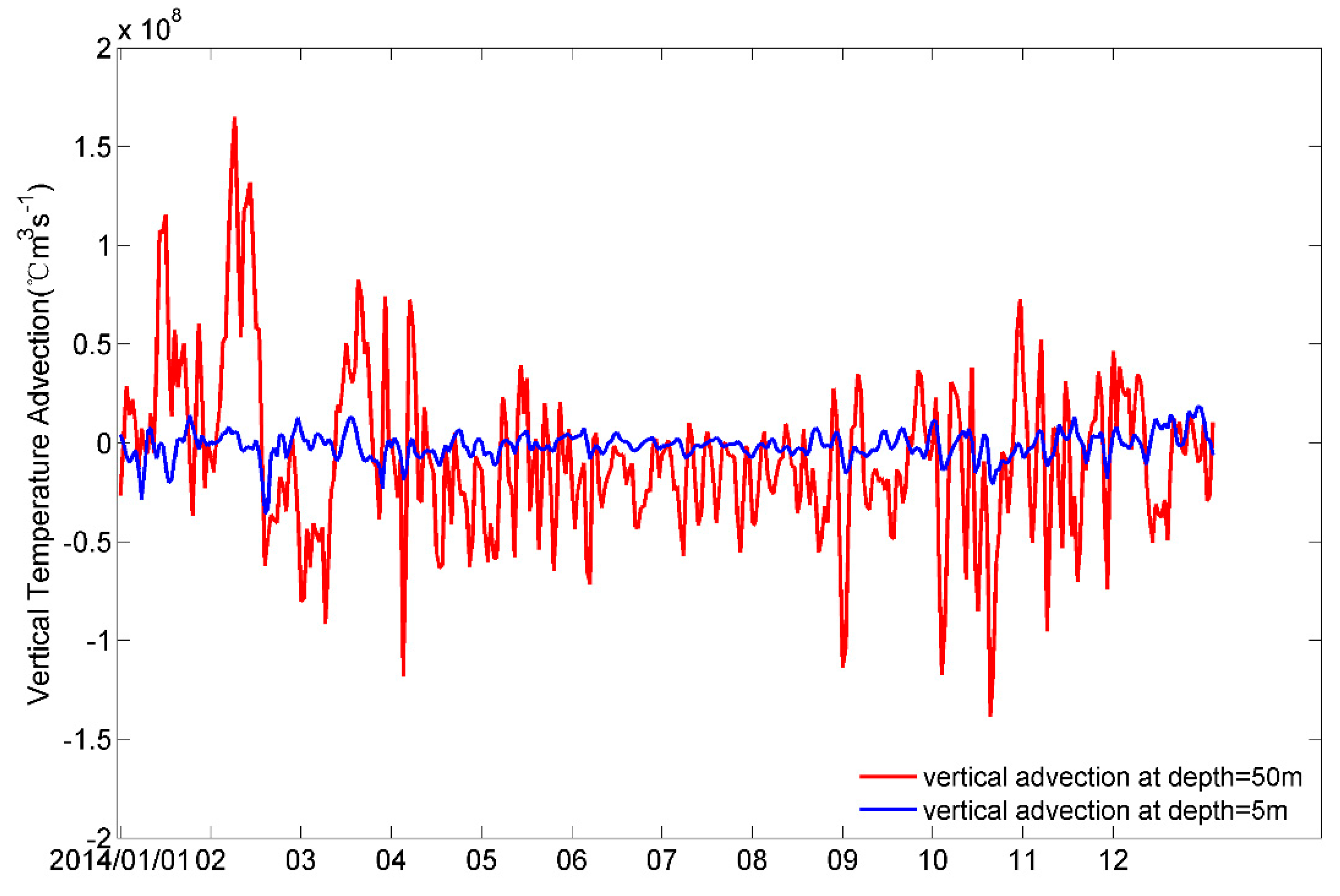
4.1. Mixed Layer Budgets of Temperature

To further understand what physical processes affect the SST variation in the MC, we examined the temperature budget in the mixed layer. The temperature budget equation (see details in Appendix A) is:

$$T_t=T_{hadv}+T_{zadv}+T_{hdiff}+T_{zdiff}+T_{wflux}$$

(4)

where $T_t$ is the temperature variation rate term on the left hand side of the equation. $T_{hadv}$ and $T_{zadv}$ are horizontal and vertical temperature flux terms, respectively, and the sum of these two terms is the temperature flux term $T_{flux}$. $T_{hdiff}$ and $T_{zdiff}$ are horizontal and vertical eddy diffusion terms, respectively, and the summary of these two terms is the total eddy diffusion term $T_{diff}$. The eddy diffusion terms typically refer to the parameterization of subgrid processes in the model (i.e., the stirring effects of small-scale eddies not resolved by the model). $T_{wflux}$ is the surface net heat flux term.

To calculate the temperature budget, we conducted a volume-integration (Equation (4)) in a fixed box. The depth of 50 m was chosen to be the bottom of the fixed box. According to previous studies [26] mentioned above, the mixed layer depth inside the MC is approximately in the range of 10–50 m. The depth 50 m of the box model includes the upper mixed layer. There are four open boundaries: the sea surface, 50 m level, section A1B1 and section A2B2 (see Figure 1). Other boundaries (section A1A2 and section B1B2) are solid, with no advection across these sections.

Figure 10a shows the contributions of three parts (total eddy diffusion term $T_{diff}$, net surface flux term $T_{wflux}$ and temperature flux term $T_{flux}$ to the temperature variation rate term $T_t$ inside the MC. It is clearly shown that temperature decreases during austral winter (from April to June) and sharply increases during spring and summer (from January to March and from August to December). $T_{diff}$ term acts as a heating force throughout the year with its lowest contribution observed in April. There is a high correlation coefficient (0.9) between $T_{diff}$ and $T_t$. As mentioned in Section 3.2.2, the surface heat flux has seasonal variation. In austral summer and winter (especially in winter), $T_{wflux}$ term plays a cooling role in $T_t$. This means the upper ocean loses heat. In other seasons, $T_{wflux}$ term plays a warming role in $T_t$. The correlation coefficient between $T_{wflux}$ term and $T_t$ is 0.8. In general, $T_{flux}$ term plays a warming role in $T_t$ (except for January and February).

Previous studies show that the Mozambique Current, a branch of the South Equatorial Current, flows into the MC, which carries warm water [31,32]. The monthly mean meridional temperature flux inside the MC is shown in Figure 10b. There is seasonal variation in the meridional heat flux: the difference in the temperature fluxes at the northern and southern boundaries resulting in the heat flux into the channel by the current advection. The Mozambique Current carries more hot water into the MC in austral summer than in other seasons because, in summer, the SST near the equator is the warmest. In summary, the hot water carried by the Mozambique Current has an influence on the warmer SST inside the MC.

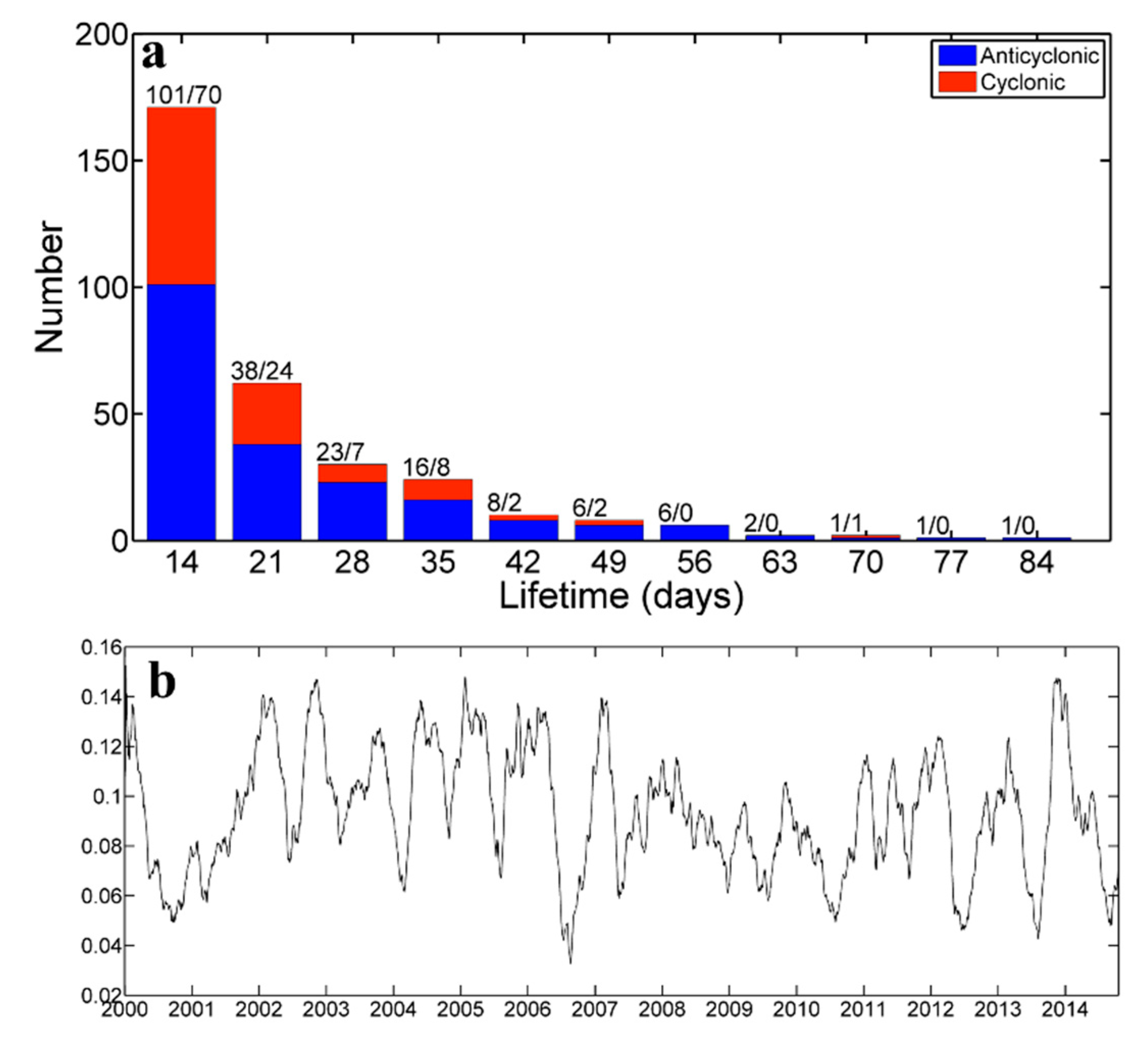
4.2. Eddies inside the MC

The eddies inside the MC also play an important role in SST anomalies inside the MC. Previous studies show that eddy activities are strong inside the MC [33,34]. We applied the eddy detection method introduced in Section 2 to the AVISO geostrophic current data from 2000 to 2014, and obtained an eddy dataset including positions, radii, lifetimes, and intensities of the eddies inside the MC. Totally, 2298 eddies (1036 cyclonic eddies and 1262 anticyclonic eddies) were identified in the 15 years. Only the eddies with a lifetime longer than 14 days (Figure 11a) were used for analysis, which reduced the impact of short-time scale factors. Figure 11a shows eddy numbers against eddy lifetime inside the MC. Most of eddies have a lifetime of less than three weeks. The anticyclonic eddy with the longest lifetime lasted over 85 days while the longest cyclonic lasted 70 days. There are more anticyclonic eddies than cyclonic eddies inside the MC in all eddy lifetime. Generally, the warm (cold) water is associated with an (a) anticyclonic (cyclonic) eddy due to the downwelling (upwelling) caused by the eddy convergence (divergence) [35]. The SST contributions (Figure 11b) from the eddies inside the MC are calculated:

$$\frac{{{\displaystyle \sum }}_{\mathrm{eddy}\mathrm{number}}\left(\mathrm{eddy}\mathrm{area}\right)\times \left(\mathrm{SSTA}\mathrm{in}\mathrm{the}\mathrm{eddy}\right)}{\mathrm{area}\mathrm{of}\mathrm{the}\mathrm{MC}}$$

(5)

The eddies inside the MC play a warming role (mean value $0.09°\mathrm{C}$) in the SST all the time. The maximum value can reach up to $0.15°\mathrm{C}$, and the minimum value is less than $0.04°\mathrm{C}$.

In summary, the background oceanic currents (the Mozambique Current and eddies) also play an important role in the warmer SST inside the MC.

5. Conclusions

In this study, both satellite remote sensing SST data and numerical model results show that the SST inside the MC is warmer than that east of the MI, which results from the presence of the MI. When the wind blows through the MI, the intensity of the wind is drastically reduced, which weakens the mixing of the upper ocean. The presence of the MI also has an important influence on the four components of heat flux, which is due to the topographic effect. Under the influence of the wind intensity and heat flux, the mixed layer depth inside the MI is shallower than that east of the MI, which means there is less cold water going upward. The correlation coefficient between the mixed layer depth and SST is −0.85. Further analysis showed that the background oceanic currents (the Mozambique Current and eddies) also play an important role in the warmer SST inside the MC.

More observation data and high-resolution models are needed to have a better understanding of mesoscale and sub-mesoscale processes in this region.

References

1. Dietrich, D.E.; Bowman, M.J.; Lin, C.A.; Mestas-Nunez, A. Numerical studies of small island wakes in the ocean. Geophys. Astrophys. Fluid Dyn. 1996, 83, 195–231. [Google Scholar] [CrossRef]
2. Aiken, C.M.; Moore, A.M.; Middleton, J.H. The non-normality of coastal ocean flows around obstacles, and their response to stochastic forcing. J. Phys. Oceanogr. 2002, 32, 2955–2974. [Google Scholar] [CrossRef]
3. Coutis, P.F.; Middleton, J.H. The physical and biological impact of a small island wake in the deep ocean. Deep-Sea Res. 2002, 49, 1341–1361. [Google Scholar] [CrossRef]
4. Barton, E.D.; Basterretxea, G.; Flament, P.; Gay Mitchelson-Jacob, E.; Jones, B.; Arístegui, J.; Herrera, F. Lee region of Gran Canaria. J. Geophys. Res.-Oceans 2000, 105, 17173–17193. [Google Scholar] [CrossRef] [Green Version]
5. Andrade, I.; Sangrà, P.; Hormazabal, S.; Correa-Ramirez, M. Island mass effect in the Juan Fernández Archipelago (33°S), Southeastern Pacific. Deep Sea Res. Part I 2014, 84, 86–99. [Google Scholar] [CrossRef]
6. Harlan, J.A.; Swearer, S.E.; Leben, R.R.; Fox, C.A. Surface circulation in a Caribbean island wake. Cont. Shelf Res. 2002, 22, 417–434. [Google Scholar] [CrossRef]
7. Neill, S.P.; Elliott, A.J. Observations and simulations of an unsteady island wake in the Firth of Forth, Scotland. Ocean Dyn. 2004, 54, 324–332. [Google Scholar] [CrossRef]
8. Dong, C.; Mcwilliams, J.C. A numerical study of island wakes in the Southern California Bight. Cont. Shelf Res. 2007, 27, 1233–1248. [Google Scholar] [CrossRef]
9. Dong, C.; Mcwilliams, J.C.; Shchepetkin, A.F. Island wakes in deep water. J. Phys. Oceanogr. 2007, 37, 962–981. [Google Scholar] [CrossRef]
10. Dong, C.; Cao, Y.; McWilliams, J.C. Island Wakes in Shallow Water. Atmos. Ocean. 2018. [Google Scholar] [CrossRef]
11. Tomczak, M. Island wakes in deep water and shallow water. J. Geophys. Res. 1988, 93, 5153–5154. [Google Scholar] [CrossRef]
12. Barton, E.D.; Flament, P.; Dodds, H.; Mitchelsonjacob, E.G. Mesoscale structures viewed by SAR and AVHRR near the Canary islands. Sci. Mar. 2001, 65, 167–175. [Google Scholar] [CrossRef]
13. Xie, S.P.; Liu, W.T.; Liu, Q.; Nonaka, M.; Hafner, J. Far-Reaching Effects of the Hawaiian Islands on the Pacific Ocean-Atmosphere System. Science 2001, 292, 2057–2060. [Google Scholar] [CrossRef] [PubMed]
14. Caldeira, R.M.; Marchesiello, P. Ocean response to wind sheltering in the Southern California Bight. Geophys. Res. Lett. 2002, 29, 13-1–13-4. [Google Scholar] [CrossRef]
15. Caldeira, R.M.; Marchesiello, P.; Nezlin, N.; Digiacomo, P.; Mcwilliams, J.C. Island wakes in the Southern California Bight. J. Geophys. Res.-Oceans 2005, 110, 1233–1248. [Google Scholar] [CrossRef]
16. Li, J.; Wang, G.; Xie, S.P.; Zhang, R.; Sun, Z. A winter warm pool southwest of Hainan Island due to the orographic wind wake. J. Geophys. Res.-Oceans 2012, 117, C08036. [Google Scholar] [CrossRef]
17. Arivelo, T.A.; Lin, Y.L. Climatology of Heavy Orographic Rainfall Induced by Tropical Cyclones over Madagascar: From Synoptic to Mesoscale Perspectives. Earth Sci. Res. 2016, 5, 146–161. [Google Scholar] [CrossRef]
18. Reynolds, R.W.; Smith, T.M.; Liu, C.; Chelton, D.B.; Casey, K.S.; Schlax, M.G. Daily high-resolution blended analyses for sea surface temperature. J. Clim. 2007, 20, 5473–5496. [Google Scholar] [CrossRef]
19. Wentz, F.J.; Gentemann, C.; Smith, D.; Chelton, D. Satellite measurements of sea surface temperature through clouds. Science 2000, 288, 847–850. [Google Scholar] [CrossRef] [PubMed]
20. Ducet, N.; Traon, P.Y.; Reverdin, G. Global high-resolution mapping of ocean circulation from TOPEX/Poseidon and ERS-1 and-2. J. Geophys. Res. 2000, 105, 19477–19498. [Google Scholar] [CrossRef]
21. Saha, S.; Moorthi, S.; Pan, H.-L.; Wu, X.; Wang, J.; Nadiga, S.; Liu, H. The NCEP Climate Forecast System Reanalysis. Bull. Am. Meteorol. Soc. 2010, 91, 1015–1057. [Google Scholar] [CrossRef]
22. Saha, S.; Moorthi, S.; Wu, X.; Wang, J.; Nadiga, S.; Tripp, P.; Ek, M. The NCEP Climate Forecast System Version 2. J. Clim. 2014, 27, 2185–2208. [Google Scholar] [CrossRef]
23. Shchepetkin, A.F.; McWilliams, J.C. The regional oceanic modeling system (ROMS): A split-explicit, free-surface, topography-following-coordinate oceanic model. Ocean Model. 2005, 9, 347–404. [Google Scholar] [CrossRef]
24. Li, J.; Liang, C.; Tang, Y.; Dong, C.; Chen, D.; Liu, X.; Jin, X. A new dipole index of the salinity anomalies of the tropical Indian Ocean. Sci. Rep. 2016, 6, 24260. [Google Scholar] [CrossRef] [PubMed] [Green Version]
25. Li, J.; Liang, C.; Tang, Y.; Liu, X.; Lian, T.; Shen, Z.; Li, X. Impacts of the iod-associated temperature and salinity anomalies on the intermittent equatorial undercurrent anomalies. Clim. Dyn. 2018, 51, 1391–1409. [Google Scholar] [CrossRef]
26. Nencioli, F.; Changming, D.; Dickey, T.; Washburn, L.; McWilliams, J.C. A Vector Geometry–Based Eddy Detection Algorithm and Its Application to a High-Resolution Numerical Model Product and High-Frequency Radar Surface Velocities in the Southern California Bight. J. Atmos. Ocean. Technol. 2010, 27, 564. [Google Scholar] [CrossRef]
27. DiMego, G.J.; Bosart, L.F. The Transformation of Tropical Storm Agnes into an Extratropical Cyclone. Part I: The Observed Fields and Vertical Motion Computations. Mon. Weather Rev. 1982, 110, 385. [Google Scholar] [CrossRef]
28. Zhang, Y.; Xu, H.; Qiao, F.; Dong, C. Seasonal variation of the global mixed layer depth: Comparison between Argo data and FIO-ESM. Front. Earth Sci. 2018, 12, 24–36. [Google Scholar] [CrossRef]
29. Schiller, A.; Oke, P.R. Dynamics of ocean surface mixed layer variability in the Indian Ocean. J. Geophys. Res.-Oceans 2015, 120, 4162–4186. [Google Scholar] [CrossRef] [Green Version]
30. Schiller, A.; Ridgway, K.R. Seasonal mixed layer dynamics in an eddy-resolving ocean Circulation Model. J. Geophys. Res.-Oceans 2013, 118, 3387–3405. [Google Scholar] [CrossRef]
31. Schott, F.; Mccreary, J.P. The monsoon circulation of the Indian Ocean. Prog. Oceanogr. 2001, 51, 1–123. [Google Scholar] [CrossRef]
32. Schott, F.A.; Xie, S.P.; Mccreary, J.P. Indian Ocean circulation and climate variability. Rev. Geophys. 2009, 47. [Google Scholar] [CrossRef]
33. Ruijter, W.P.; Ridderinkhof, H.; Lutjeharms, J.R.; Schouten, M.W.; Veth, C. Observations of the flow in the Mozambique Channel. Geophys. Res. Lett. 2002, 29, 140-1–140-3. [Google Scholar] [CrossRef]
34. Ullgren, J.E.; Aken, H.M.V.; Ridderinkhof, H.; Ruijter, W.P. The hydrography of the Mozambique Channel from six years of continuous temperature, salinity, and velocity observations. Deep Sea Res. Part I 2012, 69, 36–50. [Google Scholar] [CrossRef]
35. Sun, W.; Dong, C.; Wang, R.; Liu, Y.; Yu, K. Vertical structure anomalies of oceanic eddies in the Kuroshio Extension region. J. Geophys. Res.-Oceans 2017, 122, 1476–1496. [Google Scholar] [CrossRef]
Figure 1. Topography (unit: m) of the study area and section setting: A1-B1-B2-A2 is the area inside the channel and B1-C1-C2-B2 is the area east of the MI. The positions of the points are listed in Table 1. Current branches indicated are the South Equatorial Current (SEC), Northeast and Southeast Madagascar Current (NEMC and SEMC), East African Coastal Current (EACC) and Mozambique Current (MC).
Remotesensing 11 01112 g001
Figure 2. SST averaged over 33 years (1982–2014) from: (a) the Reynolds’ product; and (b) the ROMS results. (units:   ° C ).
Remotesensing 11 01112 g002
Figure 3. The 33-year (1982–2014) monthly averaged SST (unit:   ° C ) in the study area from the ROMS data. JAN, FEB, MAR, APR, MAY, JUN, JUL, AUG, SEP, OCT, NOV and DEC denote the months from January to December, respectively.
Remotesensing 11 01112 g003
Figure 4. (a) The difference of area-averaged SST between inside the MC and east of the MI using the ROMS results from January 1982 to December 2014 (unit:   ° C ). (b) Blue line: the monthly difference of the SST; red dotted line: mean value; shading: the standard deviation. (c) The yearly means of the above SST differences from 1982 to 2014.
Remotesensing 11 01112 g004
Figure 5. The 33-year (1982–2014) monthly averaged wind fields in the study area from the NCEP CFSR data. The vectors represent the wind direction while the wind magnitude is shown as shaded (units: m/s). JAN, FEB, MAR, APR, MAY, JUN, JUL, AUG, SEP, OCT, NOV and DEC denote the months from January to December, respectively.
Remotesensing 11 01112 g005
Figure 6. (a) Surface net heat flux (unit: Wm−2); (b) solar-wave short radiation net flux (unit: Wm−2); (c) long-wave radiation flux (unit: Wm−2); (d) latent heat flux (unit: Wm−2); (e) sensible heat flux (unit: Wm−2); and (f) liquid cloud water (unit: mm) in study area. The liquid cloud water data are from the TMI (1998–2014) and the heat flux data are from the NCEP CESF (1982–2014).
Remotesensing 11 01112 g006
Figure 7. Schematic diagram of influencing factors of the temperature in the mixing layer.
Remotesensing 11 01112 g007
Figure 8. The 33-year (1982–2014) monthly averaged surface mixed layer depth in the study area from the ROMS data (units: m). JAN, FEB, MAR, APR, MAY, JUN, JUL, AUG, SEP, OCT, NOV and DEC denote the months from January to December, respectively.
Remotesensing 11 01112 g008
Figure 9. The time series of domain-averaged SST (unit:   ° C ) and surface mixed layer depth (unit: m) from 1982 to 2014 using the ROMS results inside the MC by 12-month moving smooth. Red line: SST; blue line: the mixed layer depth.
Remotesensing 11 01112 g009
Figure 10. (a) Monthly average of temperature rate of change ( T t ), total advection term ( T h a d v + T z a d v ), total diffusion term ( T h d i f f + T z d i f f ) and surface flux term ( T w f l u x ) in 2014 inside the MC (upper 50 m). (b) Monthly net meridional heat flux in 2014 inside the MC.
Remotesensing 11 01112 g010
Figure 11. (a) Histogram of eddy number per eddy lifetime. Blue for anticyclone, red for cyclone. (b) the SSTA contributions of all the eddies on the MC by 90-day moving smooth.
Remotesensing 11 01112 g011