1. Introduction
LiDAR (Light Detection and Ranging) systems are widely used in mobile and airborne mapping at various scales. Airborne surveys enable to map wide areas at high speed and relatively low resolution, while unmanned aerial vehicles (UAV) are used to get a detailed description of local areas. LiDAR systems are composed of a positioning system (GNSS receiver), an inertial measurement unit (IMU) and a LiDAR measuring relative distances to the terrain.
Georeferencing is performed by combining LiDAR angles and distance measurements, IMU attitude angles and GNSS positions with a point positioning mathematical model. This model depends on several parameters which are sources of systematic errors that can be observed by comparing overlapping survey strips [
1].
LiDAR systems geometric parameters requiring accurate calibration include LiDAR-IMU boresight angles and lever-arms between the positioning reference point (PRP) and the optical center (OC) of the LiDAR [
2]. The geometric calibration of LiDAR systems eliminates systematic errors due to boresight (i.e., angular mis-alignment between the LiDAR and IMU measurement frames) and to lever-arms i.e., translational offset between the assumed and actual vector joining the PRP and the OC (see
Figure 1 for a definition of a LiDAR system geometry).
LiDAR-IMU latency should also be considered as a source of error in LiDAR system surveys, since the time-tagging implementation may introduce offset and drift between the LiDAR time base and the IMU time base. A method for the recovery of IMU-LiDAR was proposed in [
3]. Latency calibration should be performed before boresight and lever-arms calibration to avoid the presence of dynamic errors due to latency (the which are amplified by the survey platform motion).
As uncertainty due to boresight is one of the most significant sources of non consistency between LiDAR overlapping strips [
4], a significant amount of work has been done in boresight calibration. In [
5], tie points are used to adjust the boresight angles of a LiDAR systems, which limits the method accuracy due to the need of interpolating raw data. Surface matching techniques have also been used in [
6]. The main drawback of these methods is modelling the effect of boresight as a rotation in the LiDAR object domain, which is true for points, but not for surfaces. This makes this type of method semi-rigorous. A classification between a rigorous, semi-rigorous and non rigorous method was proposed in [
7]. Rigorous methods estimate the boresight angles by adjusting a parametric model which is consistent with the actual effect of boresight on a geometrical object: if the boresight angles are represented by a rotation matrix, then the estimation should be done from data actually distorted by the same class of rotation. In fact, rigorous methods adjust a parametric model using point or swath data, as these two objects are subject to boresight rotation. Adjusting normal vectors to planes lies in the semi-rigorous class of methods, even if the plane elements are sufficiently small. Indeed, the effect of boresight error on a planar surface may not be a rotation, as shown in
Figure 2.
Extensive research has been performed in boresight calibration of LiDAR systems, leading in the recent years to rigorous methods [
1,
8,
9,
10] for boresight adjustment. In [
10] a rigorous boresight estimation method based on the adjustment of points on planar surface elements has been proposed. This method can be used whenever the underlying terrain exhibits planar regions. In [
9] a Random Sample Consensus (RANSAC)-based [
11] shape extraction method is proposed to match homologous surfaces.
Most of the approaches proposed for boresight calibration use a model of the systematic errors effect through a point georeferencing model [
7,
12,
13,
14]. By observing inconsistencies in point clouds from overlapping survey strips, an error criterion can be defined and optimized to adjust overlapping points on a given parametric surface. Boresight angles and surface parameters are then determined simultaneously by applying a least square procedure.
One of the major outcomes of automatic calibration methods lies in the statistical analysis of boresight residuals, providing precision estimates of the boresight angles adjustment. This information can then be used for quality control purposes and also to refine combined standard measurement uncertainty (CSMU) models (also call total propagated error, but we prefer the terminology CSMU which follows the International Vocabulary of Metrology [
15]), based on the propagation of each LiDAR system component uncertainty, including boresight.
This paper details a new method to estimate boresight angles for LiDAR systems which follows the same lines as these recent methods, but we propose some improvements in terms of data selection. Data selection consists of determining local planar areas by a quad-tree algorithm, whose criterion is based on the propagation of a CSMU for each LiDAR point within the normalized residual of plane parameters. This feature makes our data selection robust to the presence of irregular shapes in the calibration area. Moreover, we define a sensitivity function of planar surface element to each boresight angle that enables to select only the most relevant surface element in the boresight angles adjustment. The effect of this selection method is to maximize the information contained in each observation equation, to limit the size of the least square problem and as a result, to optimize the boresight angles observability and to improve the numerical stability and processing time of the calibration method.
The paper is organized as follows: we first discuss a general framework for system and mounting parameters of LiDAR systems. In the second section, we present the mathematical formulation of point georeferencing together with the problem setting of boresight calibration on natural surfaces. We shall show that one of the key point of boresight calibration on natural surfaces lies on appropriate data selection methods. Then, we present numerical results obtained with several datasets from different LiDAR systems integrated within a drone, and we conclude on the performances of the proposed calibration method.
2. LiDAR System Georeferencing Model And Parameter Calibration
As illustrated in
Figure 1, a typical LiDAR survey system consists of:
A positioning system giving the position of a positioning reference point (PRP), is denoted by hereafter.
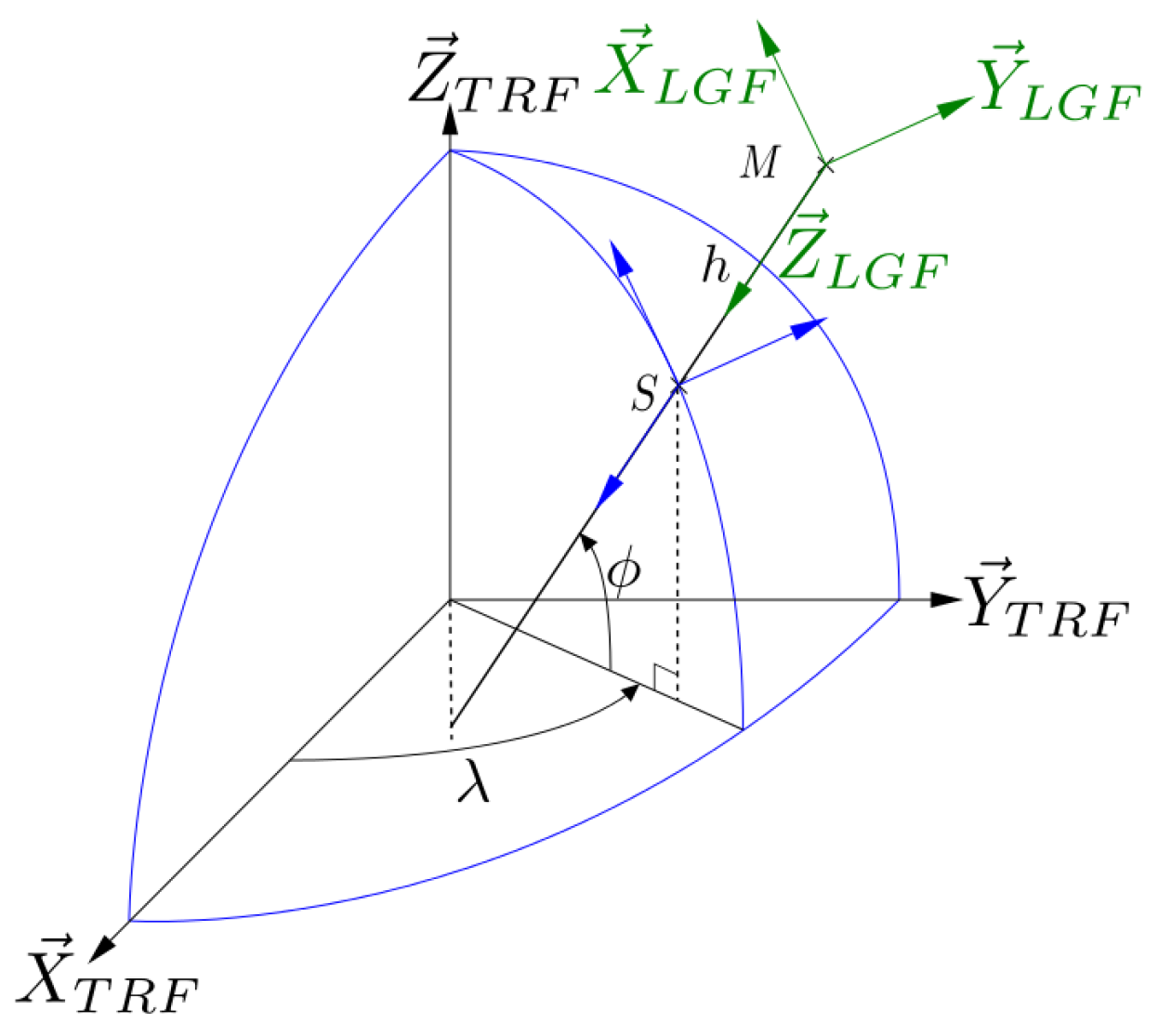
An IMU giving its orientation with respect to a local astronomic frame (LAF) (Let us mention that in practice, the IMU gives orientation in a local geodetic frame (LGF), as most IMU used in airborne surveying are not accurate enough to distinguish the LAF from the LGF. Therefore, we shall denote the LGF frame by (navigation frame) to avoid confusion between geodetic and astronomical frames.). The IMU is composed by three accelerometers and three gyrometers, eventually hybridized with the GNSS system. It delivers the three attitude angles of the IMU with respect to the LGF.
A LiDAR, delivering relative distances from the LiDAR optical center (OC) to the ground. The LiDAR output is generally given in Cartesian coordinates within the LiDAR frame.
The following frames will be used:
The LGF, that will be denoted by
and called the navigation frame (see
Figure 3). The LGF frame can be for example a North-East-down (NED) frame, the N and E axis being tangent to the Ellipsoid at a chosen reference point.
The IMU body frame, denoted by .
The LiDAR body frame, denoted by .
The objective of this paper is to design a calibration method for estimating the frame transformation from the frame to the frame, denoted by which depends on three boresight angles, denoted by the boresight roll angle, , the boresight pitch angle and , the boresight yaw angle. We shall denote hereafter by the direction cosine matrix corresponding to the transformation from frame to frame .
The data selection for the adjustment of boresight angles requires georeferenced points. Moreover, the optimization model to estimate boresight angles incorporates the georeferencing process. For a given LiDAR return, the georeferencing can be done as follows:
where
is the geo-referenced point coordinated in the frame.
, the PRP position of the survey platform coordinated in the n frame; , the longitude, the latitude and h the ellipsoidal height; obtained from the GNSS system.
is the frame transformation from frame to frame; the attitude data, respectively roll, pitch and heading given by IMU.
is the lever arms coordinated in frame.
is the frame transformation matrix from frame to ; it is the boresight matrix; are respectively the roll, pitch and yaw boresight angles.
.
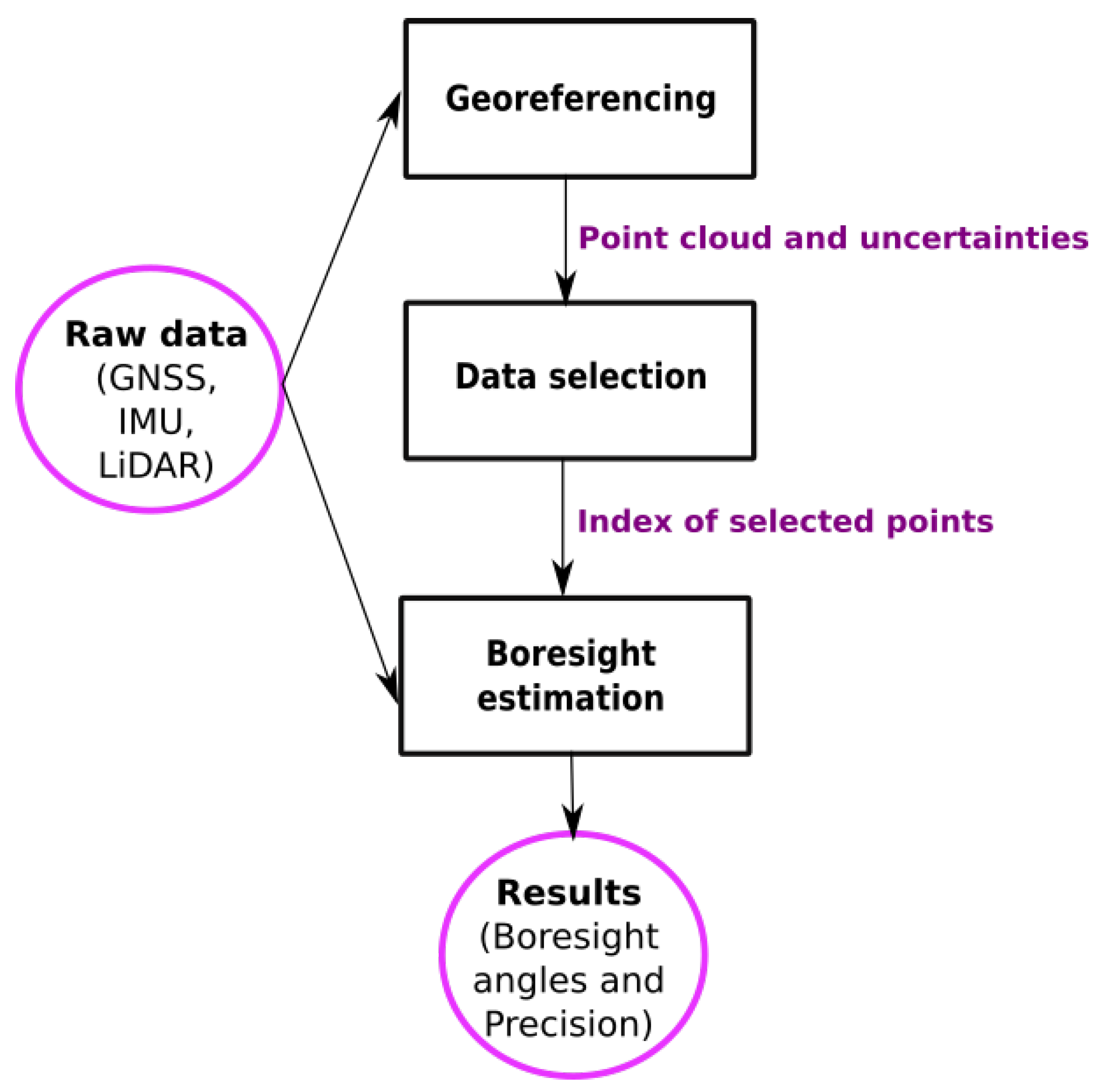
The aim of this paper is to determine the boresight transformation by an automated procedure we designed, called LiDAR IMU boresight automatic calibration (LIBAC).
LIBAC has three modules that are summarized in
Figure 4. In the next sections, we describe the data selection and the adjustment process.
LIBAC determines the boresight angles by adjusting points from several calibration lines, that should be performed by following a given set of line patterns as shown in
Figure 5:
Two parallel overlaping calibration lines oriented toward the steepest slope of a natural terrain.
Two crossing calibration lines over an area containing roofs or natural slopes.
Three crossing calibration lines over roofs or natural slopes.
These patterns are not exhaustive, the most important factors are the terrain morphology and the relative orientation of lines. The area for the acquisition of data should contain smooth and sloping surface. The calibration lines should be acquired such that the overlapping points are located within sloping surfaces elements.
The line orientations enable to observe boresight errors between calibration lines georeferenced data. The data selection method presented in
Section 3 chooses planar areas with the maximum sensitivity to boresight parameters from each calibration lines. Then, all points from the selected surface elements are fitted to the plane equations by adjusting the boresight angles, as explained in
Section 4.
3. Data Selection for Boresight Adjustment
The purpose of data selection is twofold: firstly, to extract planar areas from the calibration lines. Indeed, we shall see in the next section that the observation equation we use for boresight adjustment translates the fact that any point
(as defined by Equation (
1)) from an overlapping survey line and belonging to a planar surface element, should verify
where
.
Secondly, to select the planar surface elements having the highest sensitivity to boresight errors. Indeed, the adjustment should be performed from data exhibiting the highest boresight error, in order to maximize the input data systematic error to noise ratio and also to limit the number of variables of the boresight adjustment method.
3.1. Detection of Planar Surface Elements
Our approach follows the methods proposed in [
9,
10]. It consists to find planar surface elements for which we can observe the maximum effect of systematic error due to boresight. To be able to achieve a boresight calibration over a natural surface, we adopted a variable resolution approach based on a quad-tree decomposition [
16].
To decide if a quad-tree surface element is a plane, we use a Deming least-square (DLS) hyperplane fitting method [
17]. DLS is a non linear estimation method that enables to propagate the CSMU (While we compute points thanks to a point georeferencing model (
1), we also compute the CSMU ellipsoid of uncertainty associated to each point.) of each LiDAR points. This approach is detailed in [
18] in the general case of a set of hyperplanes. By using DLS, we can propagate the CSMU
of each individual point (Note that a classical Least Square would propagate the same Normal distribution for
all points. to the statistical parameters of the planar surface elements.). The CSMU is computed by using the estimted standard uncertainty of each sensor (GNSS, IMU, LiDAR). For the LiDAR system, ranging uncertainty and scan angle precision are generally given by the manufacturer.
We compared the results of a DLS approach to a classical principal component analysis (PCA) method [
19] and we observed that using the CSMU in input of the DLS method gives more reliable plan coefficient estimates and therefore a better segmentation of the point cloud in planar surface elements than using a PCA.
The quad-tree subdivision process termination test takes into accounts the number of points within the surface elements and also tests the presence of at least two survey strips (this enables to guarantee the use of overlapping points). Whenever the subdivision of overlapping strips in planar areas is done, we search the best surface elements to be used for boresight angles estimation. To do so, we construct a sensitivity criterion which computes the relevance of each surface element to boresight estimation. Points from the selected surface elements will be the only one used for boresight adjustment.
The outcome of the planar area detection process is a set of planar element indexes, the georeferenced points belonging to them and associated raw data (position, attitude, LiDAR return). This set of planar elements is then analyzed by the data selection process, as explained in the next section.
3.2. Boresight Sensitivity Criterion for Surface elements
We describe the selection process of the most sensitive surface elements for boresight estimation. This phase is essential to minimize the size of the underlying optimization problem of boresight adjustment (We shall see that the size of the boresight estimation problem is , where P is the number of selected surface elements.).
On each surface element
j selected by the quad-tree process, the point cloud include data from several overlapping strips. Let us consider a given planar surface element. We define
as the elevation difference between the centroid of the plane fitted with the points from all the survey strips(denoted by
) and the centroid of the plane fitted only with the points from the strip
j (denoted by
):
where:
where
are the plane coefficients adjusted with points from the strip
j,
are the plane coefficients adjusted with the point from all strips intersecting the surface element
j and
are the horizontal coordinates of the centroid of the surface element.
In order to define the sensitivity criterion, we need to express as a function of boresight angles. To do so, we introduce a virtual vector joining:
Note that this last point depends on
j as its elevation is computed using the coefficients of the plane fitted using strip
j point data, as given by Equation (
4) and can be written by:
We can also define this point using a “virtual” georeferencing equation:
where
is the average coordinate transformation matrix defined by the IMU attitudes while the surface element is reached by LiDAR points.
denotes the boresight transformation matrix. To express the virtual LiDAR return we approximate it (without the effect of boresight) by:
Then, using Equations (
5) and (
6), we construct the difference of elevation in (
3) as the function of boresight (We use the centroid of the planar elements for data selection. Let us mention that using centroids for boresight adjustment would lead to unstable boresight estimation due to irregular sampling of planar elements.)
We define the sensitivity criterion by the min-max error of the gradient of with respect to the boresight angles (i.e., the variation of due to boresight angles), over all survey strips j.
Indeed, a surface element is sensitive to boresight whenever the planar surfaces fitted from points of strip j have a significant elevation difference due to boresight variations.
3.3. Results of the LIBAC Data Selection
The results we present were obtained with the data selection module of LIBAC on a dataset acquired by a UAV from the company Microdrones (
www.microdrones.com). The drone was a MD4-1000 and was equipped with a Sick LiDAR (
www.sick.com), an Applanix APX15 GNSS/INS (Global Navigation Satellite System/Inertial Navigation System,
www.applanix.com/products/dg-uavs.htm). The survey lines were done according to a line pattern designed for calibration over natural slopes, formed by two overlapping parallel lines oriented towards the steepest slope. Note that, actually, a different line pattern can also be used successfully for LIBAC.
In
Figure 6, we show the result of the boresight sensitivity criterion computation on the quad-tree surface elements and the roll boresight sensitivity, which is clearly higher over the overlapping areas of the line pattern. As expected, the pitch boresight sensitivity was higher in slopes and close to the Nadir areas of the survey lines (see
Figure 6). The sensitivity to the yaw boresight is higher for the outer beams overlaps with significant slopes, as shown in
Figure 6.
Figure 6 bottom right shows the result of the automatic data selection performed by application of the quad-tree analysis and the sensitivity criterion defined in
Section 3.2. It can be seen that the selected areas lies on the slope, where overlapping survey lines enable both the adjustment of roll pitch and yaw boresight angles.
As the access to terrains with steep and smooth natural slopes could be constraining, it is also possible to use LIBAC on building roofs. In
Figure 7 we present an example of point cloud containing roofs, for which the LIBAC data selection were applied. This process was performed automatically and therefore do not require the user intervention to select planar areas as it usually the case for most calibration software tools.
The LIBAC data selection from the point cloud presented in
Figure 7 is depicted in
Figure 8 that shows the quad-tree as a results of the planar regions segmentation, the UAV calibration lines (in green and brown), and the planar areas colored according to their global sensitivity to boresight level. As it can be observed, the roof is selected in the direction of survey lines. This is consistent with what we would do to optimize the boresight angles observability.
Only smooth surface elements are required for an optimal boresight angles estimation. Therefore, filtering of irregular shapes (vegetation, cables, pylons, etc.) can be performed prior to the execution of LIBAC. This can be done by applying a filter based on the analysis of local PCA covariance matrix at each point: for example, the smallest eigenvalue can be used as a reliability measure of points smoothness.
3.4. Influence of the CSMU on the Data Selection
The data selection process propagates the CSMU model through the statistical parameters of the planar surface elements. In this sense, the CSMU impacts the validation process of surface elements. Indeed, we select only the surface elements such that their normalized residuals are lower than a given threshold.
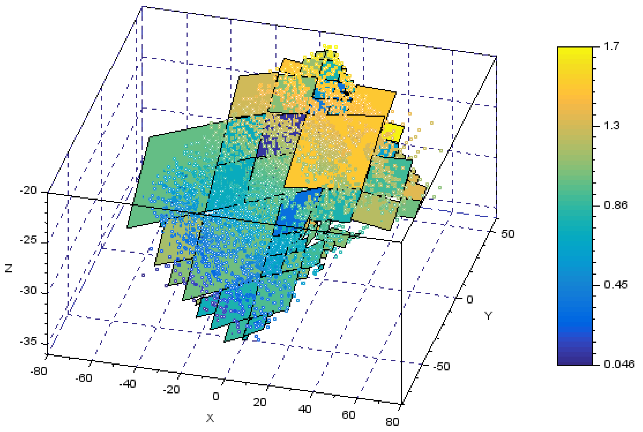
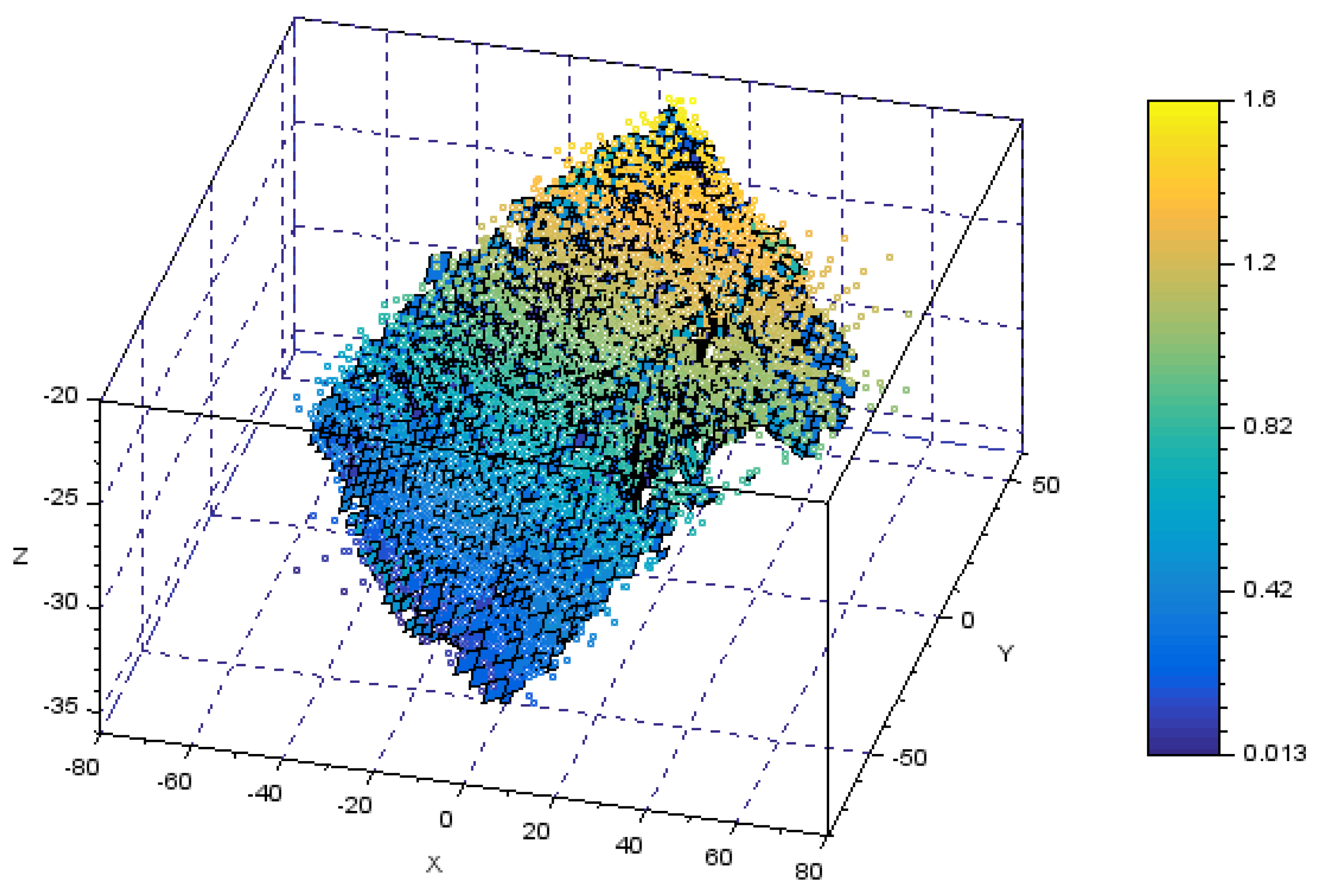
To show the relevance of the CSMU propagation in the data selection process, we ran two LIBAC sessions, enabling and disabling the CSMU computation. When we disable the CSMU, we set the CSMU of all points to a constant value. Results are shown in
Figure 9 and
Figure 10.
When the CSMU is not used, large surface elements are selected, but their size is not related to the actual level of uncertainty of their underlying point cloud. When the CSMU is taken into account, one can see that all the surface elements selected without CSMU have been unvalidated. The data selection converged toward a thin line of surface elements located in a trench. It appears that these element are sufficient to accurately estimate the boresight.
The CSMU could also have influences on the adjustment quality of boresight angles. In fact, when the CSMU computation is considered, the point cloud is well adjusted. To evaluate the consistency of the point cloud, we computed the standard deviation along surface normal (SDASN). This is done by applying a PCA within an
grid on the point cloud. The smallest eigenvalue of each cell is the point cloud orthogonal distance variance. For a dataset flown at a height of 150 m,
Table 1 summarizes the average, the maximum and the standard deviation of SDASN after applying boresight angles results of two sessions of LIBAC (by enabling and disabling the CSMU computation). As it can be observed, the CSMU computation improves the point cloud quality of two to three centimeters.
5. Numerical Results
5.1. LIBAC Efficiency
As contains P planar elements, the size of the optimization problem to be solved is . We deduce from this that the number of surface elements should be maintained as low as possible to avoid an undesirable computational time and numerical conditioning issues. The data selection process is therefore a very important component of the boresight calibration process. Its goal is indeed to select a relatively small number of planar surface elements for which the sensitivity to boresight errors is maximum.
In comparison with other methods that do not integrate any data selection, the computational time is significantly reduced (by a factor five on average). For the data set considered in
Figure 8 975 planar surface elements can be found in the calibration area and we selected only the 50 best. As a consequence, the least squares without data selection has 2928 observation equations, versus 153 with our method.
In general, the computational time we experience with LIBAC for a typical calibration data set was about 180 s on a INTEL Core i7-7700HQ (Quad-Core 2.8 GHz/3.8 GHz) processor.
Without applying the data selection, the computational time is longer, and the results accuracy is slightly reduced. Indeed, on the data set shown on
Figure 8, the boresight values found are given in
Table 2:
The difference is mainly due to the high conditioning value of the Least Square problem without data selection which make the solution more sensitive to observation uncertainty.
5.2. Results for Various Data Sets
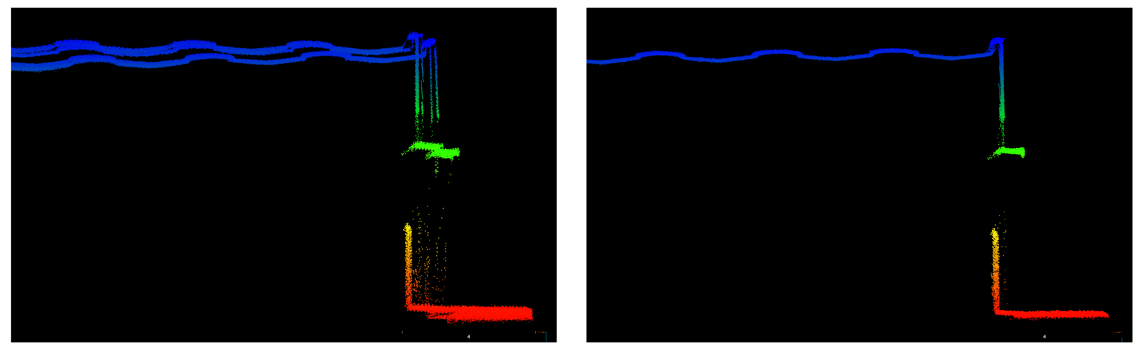
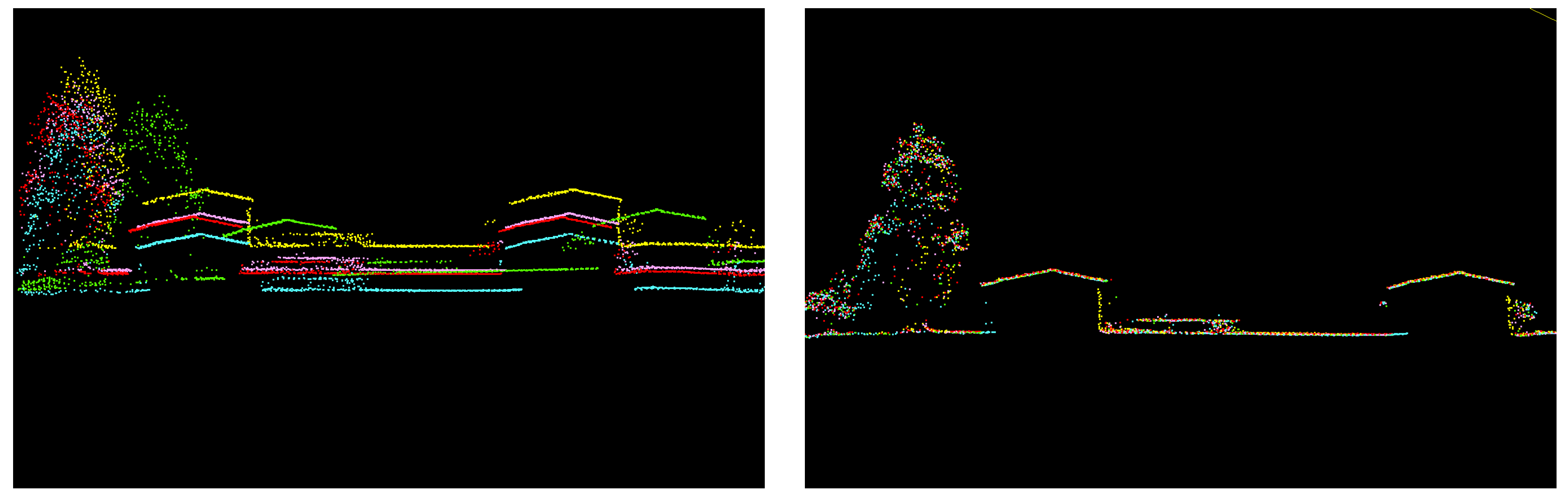
LIBAC was applied to several datasets. These datasets were acquired by systems equipped with different LIDARs (SICK, Velodyne VLP16, Riegl miniVUX-1UAV, Riegl miniVUX- DL, Riegl VUX-LR). For each dataset, the use of LIBAC improved the point cloud quality, as it can be observed from
Figure 11,
Figure 12 and
Figure 13. These figures illustrate the consistency of point clouds before and after applying LIBAC boresight angles. It is important to note that two of the datasets presented in this paper (the VUX-LR and the MiniVUX-DL datasets) were so corrupted that calibration methods from existing software were unable to estimate the correct boresight values.
For a typical dataset flown at 150 m, we computed the SDASN before and after applying boresight angles found by LIBAC. The system was constituted of a VUX-LR LiDAR and an Applanix APX20 GNSS/INS (Global Navigation Satellite System/Inertial Navigation System) and we found as boresight angles , and .
For the SDASN computation, we considered a 1 m resolution grid.
Figure 14 shows the SDASN before and after point cloud correction with LIBAC. As can be observed, LIBAC improved the point cloud quality of a few centimeters. Note that SDASN is a rigorous way to compute the point cloud “thickness”, since it takes into account the terrain local slope in contrast to standard deviation which does not.
5.3. LIBAC Consistency
The boresight estimation is said to be reproducible if for a same LiDAR system, calibration results are the same for different calibration conditions. A LIBAC reproducibility analysis was performed: ten similar pattern of lines (as illustrated to the extreme left of
Figure 5) was conducted on the same location and LIBAC results are summarized in
Figure 15. We note that, the survey conditions are different since the environmental factors are dynamic.
Datasets for reproducibility tests were acquired by a Microdrones MD4-1000 UAV, it was equiped with a sick LiDAR and an Applanix APX15 global navigation satellite system/inertial navigation system (GNSS/INS).
From the boresight angles results obtained with the ten datasets, we obtain an empirical standard deviation of , and respectively for roll, pitch and yaw boresight angles. In post-processed mode, an Applanix APX15 GNSS/INS has a roll and pitch precision of and a heading precision of . The precision of boresight angles estimation is limited by the quality of the sensors and cannot be better than the precision of the IMU. One can see that, the standard deviations of boresight angles we obtained from the ten datasets in roll and yaw are lower than the performance specifications of the used IMU. The estimated boresight angles precision may also be affected by the LiDAR data quality and this may explain the standard deviation we obtained for pitch boresight angles. However, it is not very different from the pitch IMU standard deviation.
As it can be observed in
Figure 15, we also computed the fluctuations bands for each boresight angles (delimited by red squares): we considered the sampling of boresight angles results obtained from the ten used datasets and we assumed that they follow a normal distribution. We determined the fluctuation bands at
and we observe that all the boresight angles results belong to their associated fluctuation bands.
From these analysis, reproducibility tests are validated and LIBAC can be considered as a reproducible method.
An important feature of LIBAC, as mentioned in
Section 4, is to provide the precision on the boresight angles adjustment. The estimated precision and the adjustment model can be validated by computing the normalized residuals of the optimization problem. From the statistical analysis of LIBAC boresight adjustment, we computed the normalized residuals considering each point selected to estimate the boresight angles. An histogram of the computed normalized residuals is shown in
Figure 16. It can be observed that they follow a normal distribution. This shows that the LIBAC boresight parameters estimation is unbiased. This result also prove that all the boresight systematic errors were removed.


