Scene Classification from Synthetic Aperture Radar Images Using Generalized Compact Channel-Boosted High-Order Orderless Pooling Network

Abstract

The convolutional neural network (CNN) has achieved great success in the field of scene classification. Nevertheless, strong spatial information in CNN and irregular repetitive patterns in synthetic aperture radar (SAR) images make the feature descriptors less discriminative for scene classification. Aiming at providing more discriminative feature representations for SAR scene classification, a generalized compact channel-boosted high-order orderless pooling network (GCCH) is proposed. The GCCH network includes four parts, namely the standard convolution layer, second-order generalized layer, squeeze and excitation block, and the compact high-order generalized orderless pooling layer. Here, all of the layers are trained by back-propagation, and the parameters enable end-to-end optimization. First of all, the second-order orderless feature representation is acquired by the parameterized locality constrained affine subspace coding (LASC) in the second-order generalized layer, which cascades the first and second-order orderless feature descriptors of the output of the standard convolution layer. Subsequently, the squeeze and excitation block is employed to learn the channel information of parameterized LASC statistic representation by explicitly modelling interdependencies between channels. Lastly, the compact high-order orderless feature descriptors can be learned by the kernelled outer product automatically, which enables low-dimensional but highly discriminative feature descriptors. For validation and comparison, we conducted extensive experiments into the SAR scene classification dataset from TerraSAR-X images. Experimental results illustrate that the GCCH network achieves more competitive performance than the state-of-art network in the SAR image scene classification task.

1. Introduction

With the rapid development of various synthetic aperture radar (SAR) sensors, large amounts of high-quality SAR remote sensing images have been produced. SAR images have the advantages of a certain penetration ability of vegetation and work in all weathers and round-the-clock [1]. These images have been widely used in land cover classification [2], marine observation [3,4], and environment projection [5]; however, characterizing SAR images effectively is still one of the most challenging tasks in these applications.

SAR image scene classification, which is a direct understanding and interpretation of SAR data [6,7], has become an important technique in the extraction of the ground objects, target recognition and so on [8]. The description of SAR images is more difficult than high-resolution optical remote sensing images. As shown in the Figure 1, speckle noise makes the extraction of discriminative descriptors difficult in SAR scene images; in particular, there are many irregular repetitive patterns which are spatially correlated in the SAR image [6]. Additionally, various kinds of objects exhibit diversified singularities which have different shapes, contours and textures in the scene image. Considering all of them, SAR image scene classification is indeed onerous.

Inspired by the great success achieved by CNN [9] in the computer vision community, the powerful feature representations learnt through CNN and the parameters enabling end-to-end optimization [10] make the characterization of SAR scene images possible. Research shows the different layers learn different levels of semantic information in the CNN [11,12]; they extract high-level semantic information from the edges and corners which are most salient in the deepest layer [13], and this high-level semantic information is helpful for SAR image scene classification. However, the standard convolution operation is performed by a fixed-size convolution kernel with a fixed step size corresponding to the feature map of the previous layer, and the obtained calculation result is also placed at a fixed position of the output; this is the same as the standard pooling operation. This has led to deep feature representation having strong global spatial information, and the geometric invariance is weak. To improve the performance of SAR remote sensing scene classification, we should globally order the spatial structure in small regions, and the spatial structure should be orderless in large regions (due to the layout differences of the scene image); however, the deep feature representation lacks the orderless feature descriptor [14]. The bag of visual words (BoVW) model [15,16,17] which produces orderless features and makes features characterize intra-class differences [18] achieves better performance on the scene classification. The famous feature coding used in the BoVW pipeline includes vector quantization (VQ) [19,20], sparse coding (SC) [21], locality-constrained linear coding (LLC) [22], super vector (SV) [23], Fisher vector (FV) [24], locality-constrained affine subspace coding (LASC) [25], and so on. All of them could generate orderless feature representation, which is helpful for improving the accuracy of scene classification.

Nowadays, more and more experts are focused on the BoVW model [26] and CNN [27] for remote sensing scene classification [28,29,30]. Cheng. et al [31] present a novel feature representation method for scene classification based on the bag of convolutional features (BoCF) which generates visual words from deep convolutional features using convolutional neural networks. Yuan. et al [32] obtain more discriminative deep features than direct extraction from the top convolutional layers of CNN, and the final feature representations are obtained by the LASC pooling of deep features. Meanwhile, Banerjee. et al [33] present a pattern mining-based approach for the efficient discovery of mid-level visual elements, which highlights the correlations between such local descriptors and the classes efficiently. Although these works have shown their powerful feature representation in remote sensing scene classification, they still have some shortcomings: (1) only the first-order orderless feature is considered, while high-order orderless feature representation, which can better characterize the distributions of SAR scene images, is missed; (2) the parameters of the BoVW model do not enable end-to-end optimization to make the model less flexible; and (3) the channel information of the feature descriptor is fixed in the BoVW model to make the feature descriptors less discriminative for the classification.

To solve the above issues, a generalized compact channel-boosted high-order orderless pooling network (GCCH) is presented. The proposed GCCH network can generate a compact channel-boosted high-order orderless feature descriptor, which is low-dimensional but has high discrimination; additionally, the parameters enable end-to-end optimization. The overall framework of the proposed network is illustrated in Figure 2.

The main contributions of this paper are summarized below.

• We present a generalized compact channel-boosted high-order orderless pooling network (GCCH) which learns the high-order vector of parameterized locally constrain affine subspace coding by a kernelled outer product. It enables low-dimensional but highly discriminative feature descriptors, and the dimension of the final feature descriptors can be set by us.
• We employ the squeeze and excitation block to learn the channel information of the parameterized LASC statistic representation by explicitly modelling the interdependencies between channels; the block obtains the importance of each feature channel by the adaptive learning network.
• All of the layers can be trained by back-propagation, and some important parameters on the proposed network are made to obtain better experimental parameter settings, and research on the SAR image scene classification dataset demonstrates the competitive performance.

The remainder of the paper is organized as follows: Section 2 discusses the traditional LASC method; the generalized compact channel-boosted high-order orderless pooling network is proposed in Section 3; comprehensive experimental results are reported in Section 4; and Section 5 concludes the paper and proposes future research work.

2. Traditional LASC Method

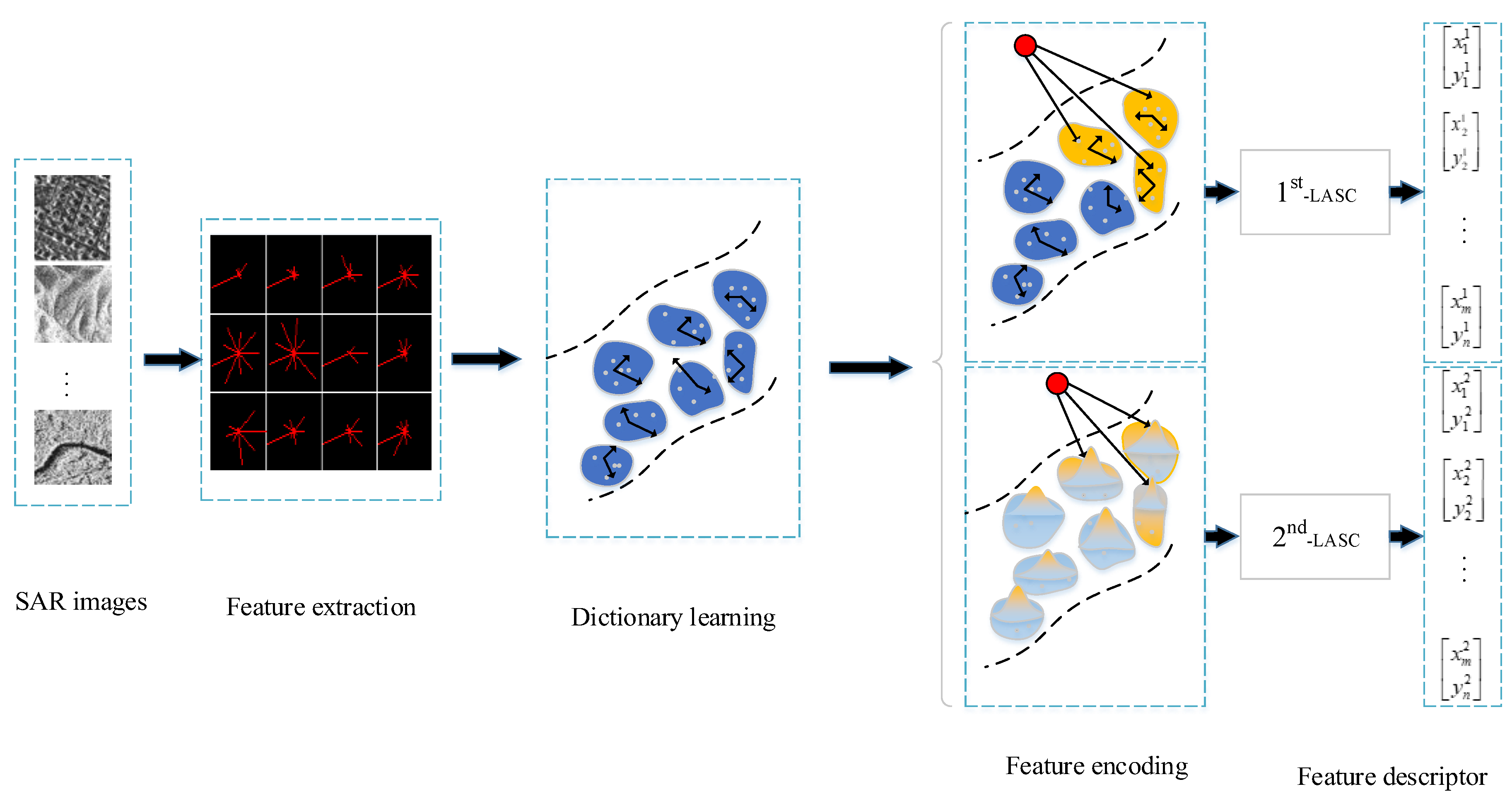
In the past decade, the bag of visual words model has played an important role in a variety of vision tasks. The standard BoVW pipeline [34,35] consists of feature extraction, dictionary learning, feature coding and spatial aggregation, and classification. Locality-constrained affine subspace coding (LASC), which is part of the BoVW model, performs first-order coding over a dictionary of affine subspaces and second-order coding based on information geometry, which has proven helpful to improve classification accuracy. Figure 3 gives the illustration of the traditional LASC method.

In the traditional LASC method, the geometry of the feature space is represented by an ensemble $S$ of low-dimensional subspace $S_i$ [25],

$$S_{\mathbf{i}}=\left\{{\mu }_i+A_i{c}_i,c_i\in R^p\right\},i=1,\dots ,\mathrm{M}$$

(1)

where ${\mu }_i$ is the attachment point of the ith subspace, which is the cluster center obtained by the $K$-means algorithm. The columns of $A_i$ ($D\times p$ matrix, $D$ is the feature dimension, $p$ is the dimension of the subspace) form an orthogonal basis of the linear subspace. $S_i$ defines a local coordinate system, and all of $S_i$ constitutes an approximation of the feature distribution actually.

The principle of LASC encoding for feature $y$ is to express the nearest top-k affine subspace, while using the neighboring metric constraint feature to project the projection vector in each neighbor affine subspace. Then, the objective function of LASC is formulated as

$$\underset{\forall c_i}{{\displaystyle \min }}{\displaystyle \sum _{S_i\in {\mathrm{N}}_k^S\left(y\right)}\left\{{\Vert \left(y-{\mu }_i\right)-A_i{c}_i\Vert }_2^2+\lambda d\left(y,S_i\right){\Vert c_i\Vert }_2\right\}}$$

(2)

where $\lambda >0$ is the parameter of the regular item. Let ${\mathrm{N}}_k^S\left(y\right)$ be the set of k, which is the closest subspaces of $y$ ; $d\left(y,S_i\right)$ denotes the proximity measure between $y$ and $S_i$, and ${\Vert •\Vert }_2$ denotes the ${\ell }_2$-norm. Based on reconstruction error, $d\left(y,S_i\right)$ is defined as

$$d\left(y,S_i\right)=\frac{\exp \left(-\gamma {\Vert \left(y-{\mu }_i\right)-A_i{c}_i\Vert }_2^2\right)}{{\displaystyle {\sum }_{i^{\prime }\in N_k^S\left(y\right)}\exp \left(-\gamma {\Vert \left(y-{\mu }_{i^{\prime }}\right)-A_i{c}_{i^{\prime }}\Vert }_2^2\right)}}$$

(3)

where $d\left(y,S_i\right)$ is defined as the exponentiated Euclidean distance, and $\gamma$ is obtained by cross-validation. We solve Equation (2) and obtain the closed-form solution of LASC, named $c_i$. Finally, cascading the feature coding of each subspace, its first-order LASC vector takes the following form:

$$c=\left[\omega \left(y,S_1\right)c_1^T,\dots ,\omega \left(y,S_i\right)c_i^T,\dots ,\omega \left(y,S_M\right)c_M^T\right]$$

(4)

where $\omega \left(y,S_n\right)={\left(1+\lambda d\left(y,S{}_n\right)\right)}^{-1}$. In particular, we can derive the second-order coding form of LASC by the Fisher information, then define the gradient vector of the likelihood function as

$$g_{S_i}={\nabla }_{S_i}\log p\left(z_i|S_i\right)$$

(5)

where $p\left(z_i|S_i\right)$ is the log-likelihood function of $z_i$, and then the Fisher information metric is

$$G_{S_i}=E_{p\left(z|S_i\right)}\left[g_{S_i}{g}_{S_i}^T\right]$$

(6)

where $E(•)$ denotes expectation with respect to $p\left(z_i|S_i\right)$. Lastly, based on Fisher’s information theory, the Fisher vector of $z_i$ is defined as

$$f_{S_i}=G_{{}_{S_i}}^{-1/2}{g}_{{}_{S_i}}=\frac{1}{\sqrt{2}}\left[\frac{{\left(z_{i,1}\right)}^2}{{\beta }_{i,1}}-1,\dots ,\frac{{\left(z_{i,1}\right)}^2}{{\beta }_{i,\rho }}-1\right]$$

(7)

The second-order LASC is calculated as a weighted Fisher vector, which is formulated as

$$f={\left[\omega \left(y,S_1\right)f_{S_1}^T,\dots ,\omega \left(y,S_i\right)f_{S_i}^T,\dots ,\omega \left(y,S_M\right)f_{S_M}^T\right]}^T$$

(8)

if $S_i\notin N_k^s\left(y\right),f_{S_i}=0$. Finally, we concatenate the first and second-order LASC statistical information, and we will acquire the entire LASC feature representation.

3. Generalized Compact Channel-Boosted High-Order Orderless Pooling Network

In this section, the proposed GCCH network will be presented in detail. As illustrated in Figure 2, the proposed network includes four parts: (1) the standard convolution layers, (2) the second-order generalized layer (parameterized LASC layer), (3) the squeeze and excitation block, and (4) the compact high-order generalized orderless pooling layer.

Table 1. The differences between the proposed GCCH network and other approaches.

Method	Include Layers	Channel Learning	High-Order Feature	Parameters Learning	Feature	End to end Training
Traditional LASC [25]	\	\	No	No	hand crafted	No
BoCF [31]	\	\	No	No	deep feature	No
NetVLAD [37]	VLAD [38] (first-order)	No	No	Yes	deep feature	Yes
GCCH (Ours)	LASC (second-order)	Yes	Yes	Yes	deep feature	Yes

gives the differences between the GCCH network and other approaches. The GCCH network learns the powerful high-order deep feature vector and the channel information by end-to-end training; additionally, the low-dimensional feature descriptor is produced to reduce the redundancy of the high-order feature vector.

3.1. The Second-Order Generalized Layer (Parameterized Lasc Layer)

First of all, the closed-form solution of Equation (2) takes the following form:

$$c_i={\left(A_i^T{A}_i+\lambda I\right)}^{-1}{A}_i^T\left(y-{\mu }_i\right)$$

(9)

where ${\left(A_i^T{A}_i+\lambda I\right)}^{-1}$ is the hard assignment coefficient; according to Equation (3), we replace it with a soft assignment coefficient [37,39],

$${\kappa }_i=\frac{e^{-\beta {\Vert y_i-{\mu }_i\Vert }_2^2}}{{\displaystyle \sum _{k^{\prime }=1}^K{e}^{-\beta {\Vert y_i-{\mu }_{k^{\prime }}\Vert }_2^2}}}$$

(10)

where $\beta$ is a positive constant, $K$ is the number of visual words (cluster centers [40]). After expanding the squares, the soft assignment coefficient can be expressed as

$${\kappa }_i=\frac{e^{w_k^T{y}_i+b_k}}{{\displaystyle \sum _{k^{\prime }=1}^K{e}^{w_{k^{\prime }}^T{y}_i+b_{k^{\prime }}}}}$$

(11)

where $w_k=2\beta {\mu }_i$, and $b_k=-\beta {\Vert {\mu }_i\Vert }^2$. LASC is a localized and second-order coding method and only considers the nearest top-k affine subspace. The soft-assignment coefficient of LASC layer is given by

$${\kappa }_i=\{\begin{array}{cc}\frac{e^{w_k^T{y}_i+b_k}}{{\displaystyle \sum _{k^{\prime }\in N_{T\left(y_i\right)}}{e}^{w_{k^{\prime }}^T{y}_i+b_{k^{\prime }}}}},& k\in N_T\left(y_i\right)\hfill \\ 0& ,\mathrm{otherwise}\hfill \end{array}$$

(12)

where $N_T\left(y_i\right)$ (T nearest neighbor layer, TNN layer) denotes the indexes of T nearest neighbor visual word of $y_i$ which is based on Equation (3). Meanwhile, the dimension of dictionary $A$ is reduced by the affine subspace layer which is based on the nearest neighbor principal component analysis (PCA) basis, and the projective matrix is defined by $P_i$ ($P_i\in R^{S\times D}$), and $S$ is the dimensionality of the subspace. The forward computation of the first-order LASC feature representation is written as

$$L^1={\displaystyle \sum _{i=1}^M{\kappa }_i{P}_i\left(y_i-{\mu }_i\right)}$$

(13)

where M denotes the number of the feature descriptors. Different from NetVLAD and LLC, LASC utilizes the second-order statistical information, according to Equation (7), and after a series of simple transformations, the forward computation of the second-order LASC statistical information is given by

$$L^2={\displaystyle \sum _{i=1}^M{\kappa }_i\left[{\left(P_i\left(y_i-{\mu }_i\right)\right)}^2-1\right]}$$

(14)

We will acquire the final LASC feature representation by cascading both $L^1$ and $L^2$ ; the network architecture of parameterized LASC layer is shown in Figure 4.

Firstly, the deep feature is normalized by $l_2$-Norm (element-wise normalization). According to Equation (11), $w_k^T{y}_i+b_k$ can be viewed as the $1\times 1$ convolution layer with the weight $\left\{w\right\}$ and bias $\left\{b\right\}$ which are well known in CNN; the exponential layer is employed to calculate $e^{w_k^T{y}_i+b_k}$, which is similar to the softmax layer. The TNN layer only considers the $T$ nearest neighbor visual word of $y_i$ ; if it is other than 0, we can implement it by the variant of the max pooling layer. The sum-norm layer is calculated by Equation (12).

The affine subspace layer is defined as the $1\times 1$ convolution layer with the weight $\left\{P\right\}$ and bias $\left\{-P\times \mu \right\}$, which is based on $P_i\left(y_i-{\mu }_i\right)$ in Equation (13), and we will acquire the first-order LASC feature representation through the product of the soft assignment layer and affine subspace layer. As seen in Equations (13) and Equation (14), the second-order LASC can be viewed as the nonlinear active function of first-order LASC; we define the activation function as $\phi \left(x\right)=x^2-1$ in the activation layer, and the derivative of $\phi \left(x\right)$ can be easily obtained. Then, the second-order statistic information is obtained. Lastly, we cascade them to acquire the final LASC statistic information. Here, all of the parameters ($\left\{w\right\}$, $\left\{b\right\}$, $\left\{P\right\}$ and $\left\{-P\times \mu \right\}$) can be trained by back-propagation in the parameterized LASC layer. Then, the algorithm steps (forward computation) of the parameterized LASC layer are given as follows:

Input: the output of the convolution $u$

Output: the entire LASC statistic information

Step1.

Normalize $u$ by the $l_2$-norm layer.

Step2.

The first-order LASC static information $L^1$ is obtained by rescaling the output of the soft assignment layer with the affine subspace layer.

Step3.

The second-order LASC static information $L^2$ is obtained by rescaling the output of the soft assignment layer with the affine subspace layer and activation layer.

Step4.

Cascading both $L^1$ and $L^2$.

3.2. Squeeze and Excitation Block

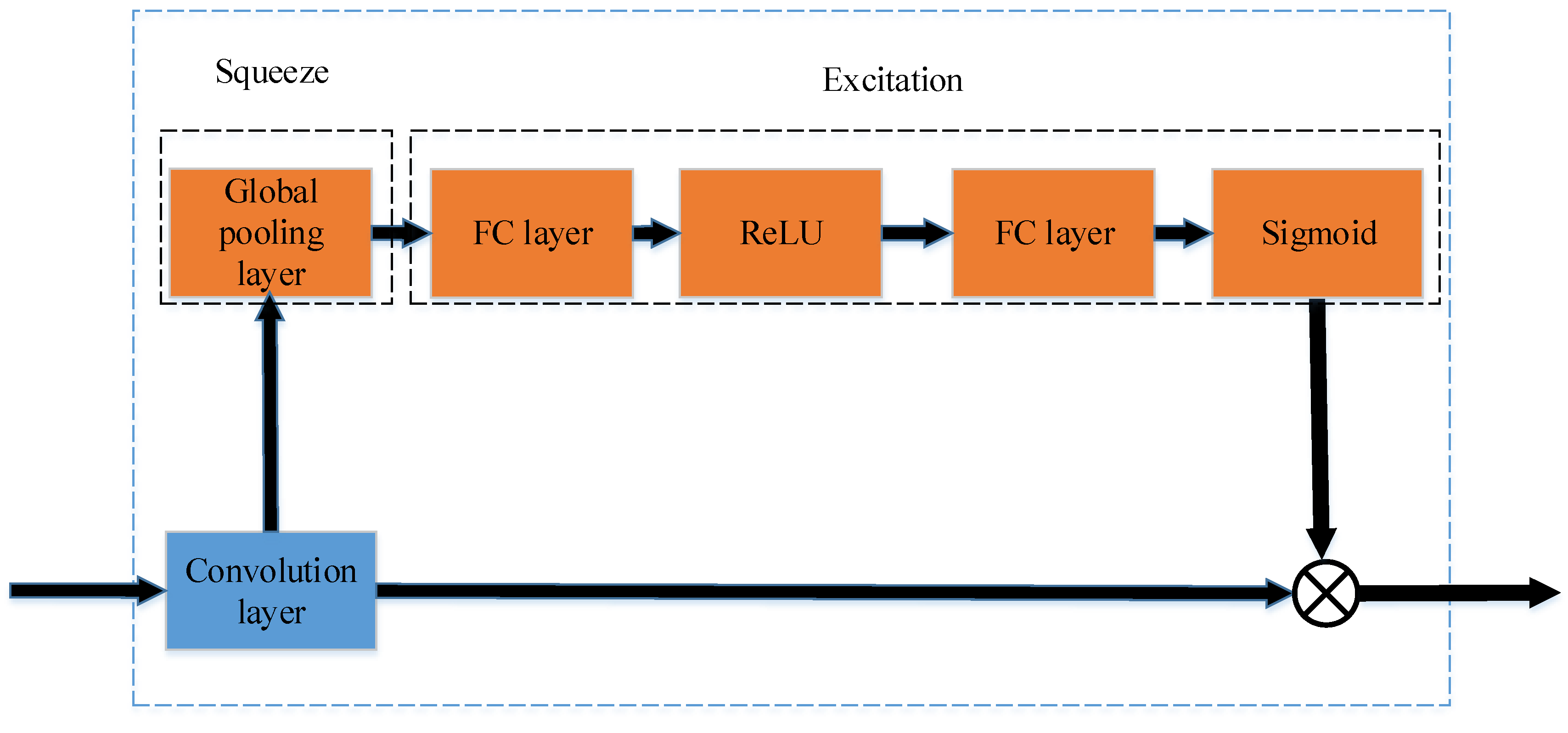
The channel information of the feature descriptor is fixed in the popular BoVW model; this makes the feature descriptors less discriminative for the classification. In order to overcome this shortcoming, the squeeze and excitation block is employed to learn the channel information of each second-order feature statistic representation [41] by explicitly modelling the interdependencies between channels; it can obtain the importance of each feature channel by an adaptive learning network. According to this, we should enhance the powerful features and suppress the features which are not helpful for SAR image scene classification. Figure 5 reports the schematic of the squeeze and excitation block.

The squeeze operation is used to generate the channel-wise statistics by using the global average pooling operation after the convolution layer, so that the feature maps ($H\times W\times C$) become the real number series of $1\times 1\times C$. $z$ is defined as the output of squeeze operation, and the $c^{th}$ element of $z$ is given by

$$z_c=\frac{1}{H\times W}{\displaystyle \sum _{i=1}^H{\displaystyle \sum _{j=1}^W{u}_c}}\left(i,j\right)$$

(15)

where $u$ denotes the output of the convolution layer. The convolution layer can be viewed as the collection of local descriptors, and the global average pooling layer makes the descriptors have a global receptive field.

The excitation operation employs the simple gating mechanism to learn the channel-wise statistics of features automatically. The excitation operation employs two fully connected (FC) layers [42] (both of which are $1\times 1$ convolution layers) and an ReLU activation layer to limit the complexity and generalization of the model, which can be shown as

$$e=\sigma \left(W_2\delta \left(W_{1}z\right)\right)$$

(16)

The first FC layer is named the dimensionality-reduction layer [43] ($W_1\in {ℝ}^{\left(C/r\right)\times C}$, $r$ is ratio of dimension reduction), $\delta$ is the ReLU activation function, the second FC layer is named the dimensionality increasing layer with parameters $W_2$ ($W_2\in {ℝ}^{C\times \left(C/r\right)}$) in the Figure 5, and $\sigma$ is the sigmoid activation function and obtains the final channel-wise statistics ($1\times 1\times C$). The algorithm steps (forward computation) of the squeeze and excitation block are illustrated as follows:

Input: the output of the convolution $u$

Output: the channel information of parameterized LASC statistic representation

Step1.

The squeeze operation $z$ is calculated by Equation (15).

Step2.

The excitation operation $e$ is obtained by Equation (16).

Step3.

Then, the output ($H\times W\times C$) is obtained by rescaling the convolution output $u$ with $e$.

The squeeze and excitation block learns the channel information of the parameterized LASC statistic representation by explicitly modelling the interdependencies between channels, and helps to boost feature discriminability.

3.3. Compact High-Order Generalized Orderless Pooling Layer

The high-order orderless feature descriptor is obtained by the kernelled outer product at a single spatial location; compared with the outer product [44,45], it enables low-dimensional but highly discriminative feature descriptors. Given the input of the compact high-order generalized orderless pooling layer $X=\left(x_1,\dots ,x_{\left|S\right|},x_s\in {ℝ}^c\right)$, $S$ is the set of spatial locations, and the fully bilinear pooling ($c\times c$ matrix) can be shown as

$$\begin{array}{cc}\hfill \langle B\left(X\right),B\left(X\right)\rangle & =\langle {\displaystyle \sum _{s\in S}{x}_s{x}_s^T,{\displaystyle \sum _{s\in S}{x}_s{x}_s^T}}\rangle \hfill \\ & ={\displaystyle \sum _{s\in S}\langle x_s{x}_s^T,x_s{x}_s^T\rangle }\hfill \\ & ={{\displaystyle \sum _{s\in S}\langle x_s,x_s\rangle }}^2\hfill \end{array}$$

(17)

where $\langle •\rangle$ is the inner product operation; the fully bilinear descriptors are a second-order polynomial kernel, and it is possible to find low-dimensional bilinear descriptors. Let $k\left(x,x\right)$ denote the kernel function, and $\langle \varphi \left(x\right),\varphi \left(x\right)\rangle \approx k\left(x,x\right)$, $\varphi \left(x\right)\in {ℝ}^d，d<c^2$. Equation (17) can be approximated by

$$\begin{array}{cc}\hfill \langle B\left(X\right),B\left(X\right)\rangle & ={{\displaystyle \sum _{s\in S}\langle x_s,x_s\rangle }}^2\hfill \\ & \approx {\displaystyle \sum _{s\in S}\langle \varphi \left(x\right),\varphi \left(x\right)\rangle }\hfill \\ & =\langle C\left(X\right),C\left(X\right)\rangle \hfill \end{array}$$

(18)

where $C\left(X\right)$ is the compact high-order orderless feature descriptor; we utilize the random maclaurin (RM) projection approach [46] to approximate these operations. The forward computation of the compact high-order generalized orderless pooling layer is given in the following steps:

Input: the output of second-order generalized orderless pooling layer $x$

Output: the compact high-order orderless feature representation $\varphi \left(x\right)$

Step1.

Generate random $W^1,W^2\in {ℝ}^{d\times c}$ (the parameters needed to be learned), and make each entry be either $+1$ or $-1$ with equal probability.

Step2.

Let $\varphi \left(x\right)=\frac{1}{\sqrt{d}}\left(W^{1}x\right)\circ \left(W^{2}x\right)$, and $\circ$ denotes element-wise multiplication.

Especially, the back-propagation of the compact high-order generalized orderless pooling layer takes the following form:

$$\begin{array}{l}\frac{\partial L}{\partial x_s^n}={\displaystyle \sum _d\frac{\partial L}{\partial y_d^n}}{\displaystyle \sum _k\langle W_k\left(d\right),x_s^n\rangle }{W}_{k^{\prime }}\left(d\right)\\ \frac{\partial L}{\partial W_k\left(d\right)}={\displaystyle \sum _n\frac{\partial L}{\partial y_d^n}}{\displaystyle \sum _s\langle W_{k^{\prime }}\left(d\right),x_s^n\rangle x_s^n}\end{array}$$

(19)

where $L$ denotes the loss function, $d$ means the projected dimension, $n$ is the index of the training sample, $S$ is the spatial index, $y_d^n$ denotes the output of the compact high-order generalized orderless pooling layer at dimension $d$—for instance $n$. $k=1,2,k^{\prime }=2,1$ —and $W_k\left(d\right)$ is the $d^{th}$ row of $W_k$. Here, the compact high-order generalized orderless pooling layer can be trained by the chain rule, and the parameters can be updated by back-propagation.

4. Experimental Results and Discussion

The challenging SAR dataset used for evaluating the proposed network is first given in this section. Subsequently, the experimental setup and experimental results for SAR image scene classification are discussed.

4.1. Date Set

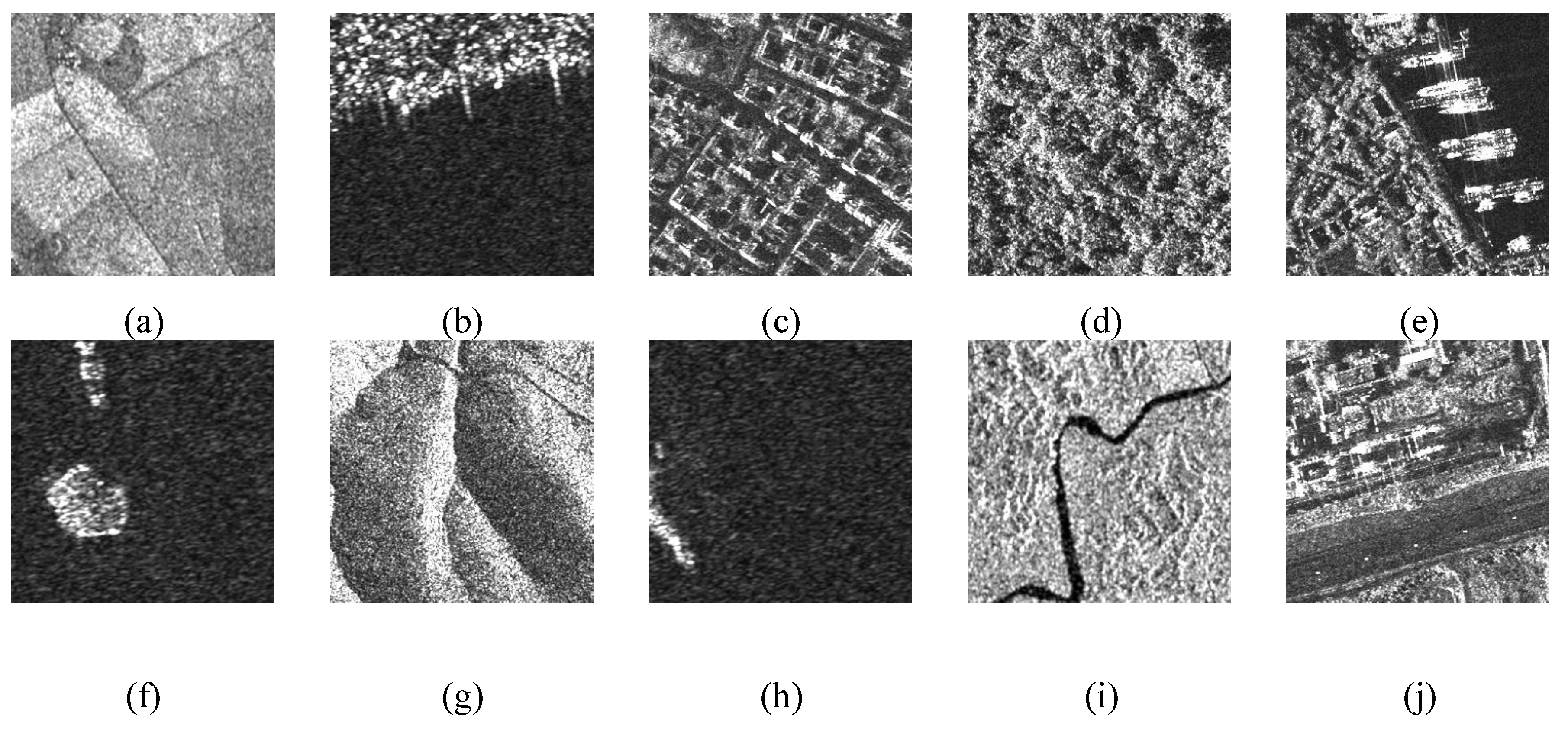
The evaluation of the GCCH network is tested on the TerraSAR-X database; this dataset contains 5000 scene images from 10 classes (agricultural, beach, building, forest, intersection, island, mountain, ocean, river, and runway), and each class consists of 500 images with the size of $256\times 256$. Example images from the 10-class TerraSAR-X dataset are shown in Figure 6.

4.2. Experimental Setup

To demonstrate the effectiveness of the GCCH network, we truncate the conv5_3 layer of VGG-16 net as the standard convolution layers, which can be downloaded from http://www.vlfeat.org/matconvnet/pretrained. The parameters of the LASC layer are set as follows: the dimension of each subspace (subspace dimension) is set to be 256, the number of subspaces (dictionary size) is fixed at 128, and k = 5 (the number of nearest subspaces). The simulations of all the methods were carried out in Matlab R2016b on the PC with Intel Core i7-8700K @3.70Ghz/16.00 GB RAM and NVIDIA 1070ti GPU; the average results are given in the following section.

For the TerraSAR-X dataset, we set the ratios of the training set to 10%, 20% and 30% (which is randomly selected per class), and 90%, 80% and 70% for testing.

4.3. Experimental Results and Discussion

First of all, a series of experimental results are made to analyze the influence of some important parameters on the GCCH network, and then we make comparisons with other state-of-the art and mid-level feature representation approaches on the TerraSAR-X dataset.

4.3.1. Evaluation of Projected Dimensions

The GCCH network generates the high-order orderless feature representations which are parameterized by the user-defined projected dimensions $d$. We perform experiments on the TerraSAR-X dataset to investigate the parameter $d$ of the proposed network. The implementation details are as follows: the ratio of reduction $r=8$, the batch size is set to 16, the learning rates are fixed at 0.001, the momentum is set to 0.9, and the weight decay is 0.005. The Adam optimizer was employed throughout our experiments, and fine-tuned the parameters of layers from Conv4_3 and above in the proposed network. The experimental results are illustrated in Figure 7.

As shown in Figure 7, when $d=128$ or 256 or 512, the experimental results decrease significantly using the low-dimensional representation, when $d\ge 1024$, the proposed network achieves better performance than the low-dimensional representation. Additionally, $d=8192$ and $d=16384$ get the highest score. In conclusion, considering the tradeoff between the model complexity and classification accuracy, we suggest that between 1000 and 8000 feature dimensions is appropriate, and we set $d=8192$ in our paper.

4.3.2. Evaluation of the Ratio of Reduction

The ratio of reduction $r$ affects the feature channel learning of the parameterized LASC layer and the parameters of the final model; different $r$ brings different model complexity, and we set the ratio of reduction from 2 to 16 in the proposed network and make experiments on the TerraSAR-X dataset. The other parameters are set as follows: projected dimensions $d=8192$, while the batch size, learning rates, momentum and weight decay are set the same as Section 4.3.1, and we fine-tune the parameters of layers from Conv4_3 and above in the GCCH network.

In the squeeze and excitation block, the additional parameters result solely from the two FC layers and make the total network capacity increase; however, the parameters will also affect the final model accuracy. Checking in

Table 2. Evaluation of the ratio of reduction.

$\mathit{r}$	TerraSAR-X Dataset
	10% Training Ratio	20% Training Ratio	Parameters
2	92.73%	93.75%	395K
4	92.71%	93.73%	198K
8	92.70%	93.70%	100K
16	92.31%	92.89%	50K

, $r=8$, $r=4$ and $r=2$ achieve similar performances which are better than $r=16$, and the accuracy of $r=16$ has a small degree of reduction. Approximately, the parameter of $r=4$ is twice that of $r=2$, and the parameter of $r=8$ is about four times than that of $r=2$. Here, considering the tradeoff between improved performance and increased model complexity, $r=8$ is optimal in the GCCH network.

4.3.3. Comparison with Other State-of-the Art Methods

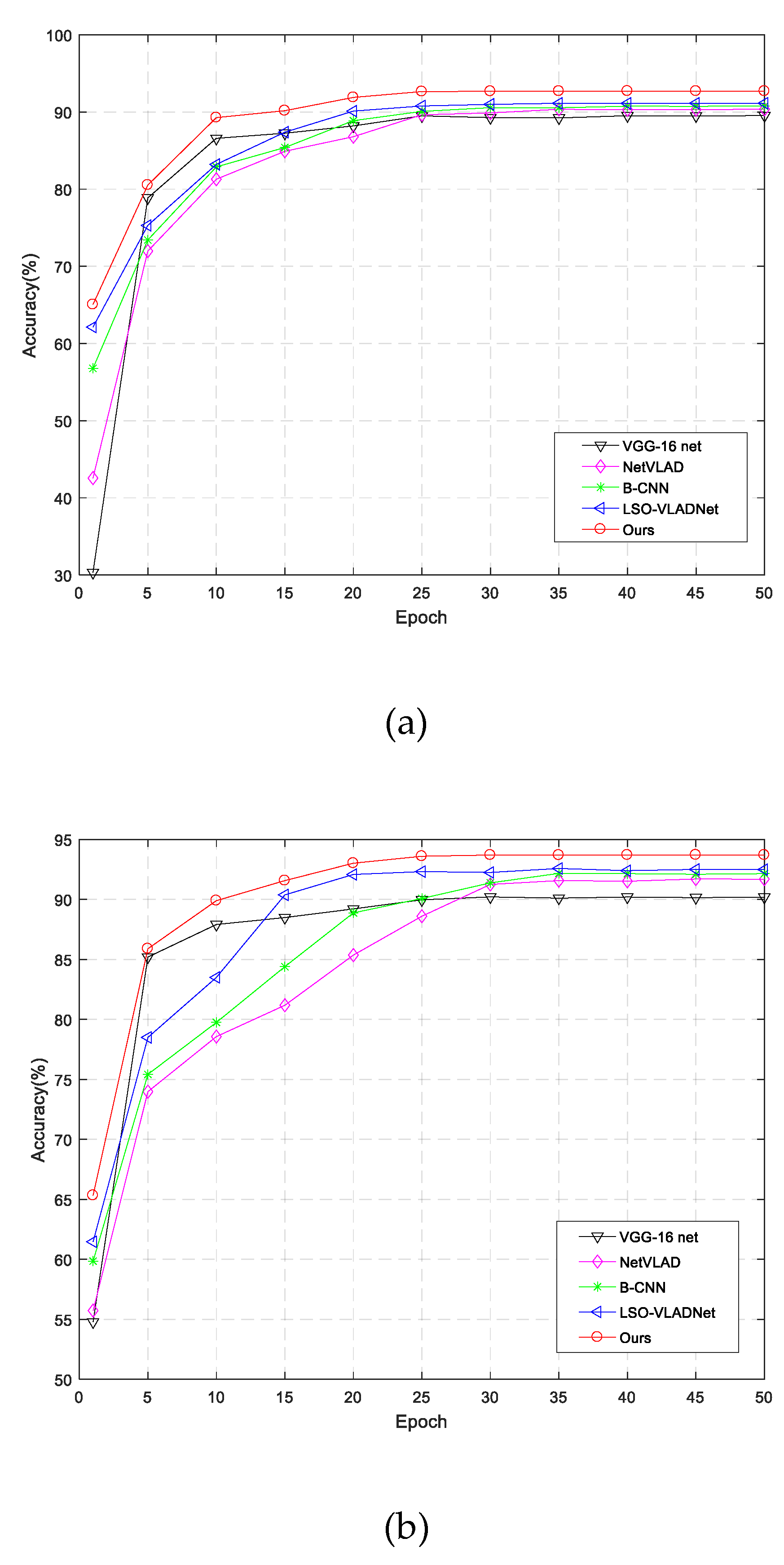
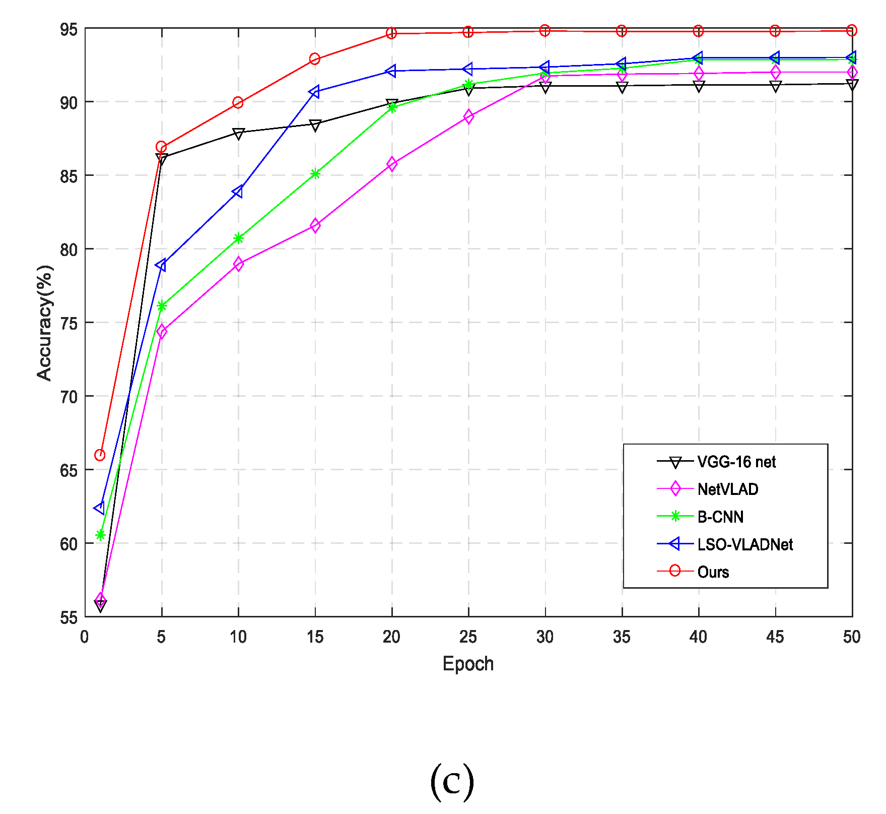
In this subsection, we make comparisons with other state of the art methods on the TerraSAR-X dataset; all the competing methods are end-to-end training (based on VGG-16 net), such as B-CNN [44], NetVLAD [37], and LSO-VLADNet [39]. For the TerraSAR-X dataset, three different training-test ratios (10%-90%, 20%-80% and 30%-70%) are set; additionally, the projected dimensions $d=8192$, the ratio of reduction $r=8$, and the other parameters are set the same as in Section 4.3.1. Figure 8 presents the performance comparisons, and

Table 3. The performance results compared with other state of the art methods.

Method	TerraSAR-X Dataset
	10%	20%	30%
ResNet-50(fine-tuning) [47]	90.10	91.28	92.23
GoogleNet(fine-tuning) [48]	89.71	90.40	91.74
VGG-16net(fine-tuning) [10]	89.53	90.21	91.23
NetVLAD [37]	90.36	91.75	92.01
B-CNN [44]	90.76	92.35	92.87
LSO-VLADNet [39]	91.14	92.58	92.91
Ours	92.70	93.70	94.80

gives the performance results (average accuracy) compared with other state of the art methods.

Because the competing methods are all based on VGG-16 net, Figure 8 only shows the comparison of VGG-16 net. As displayed in Table 3 and Figure 8, NetVLAD is a first-order generalized VLAD layer network (the feature dimension is 512), and achieves better performance than VGG-16 net (fine-tuning the last FC layer). LSO-VLADNet is a localized and second-order VLAD network and extends the novel feature coding approach to the end-to-end model (the feature dimension is 512*2=1024), and therefore it exceeds the performance of NetVLAD and VGG-16 net. The B-CNN method could acquire global feature representation using the outer product at each location of the images (we also can see it as the first-order network in our paper) and models local pairwise feature interactions in a translationally invariant manner (the feature dimension is 512*512=262144); B-CNN achieves similar performance as LSO-VLADNet, but it only considers the first-order feature representation and high dimension. The GCCH network enables low-dimensional but highly discriminative feature descriptors, which can learn the high-order of parameterized locality-constrained affine subspace coding by the kernelled outer product automatically, and the squeeze and excitation block learns the channel information of each feature representation and helps to boost feature discriminability. Therefore, the proposed GCCH network has advantages (both convergence and accuracy) over these state-of-art methods on the TerraSAR-X dataset, at about 2%-3% larger than the well-known Resnet-50, Google Net and VGG-16 net method (fine tuning).

4.3.4. Comparison with Other Mid-Level Feature Representation Methods

In this section,

Table 4. Comparison with other mid-level feature representation methods.

Method	TerraSAR-X Dataset
	10%	20%	30%
Bow [49]+SIFT [50]	80.39 ± 1.03	83.22 ± 0.53	85.06 ± 0.23
SC [21]+SIFT [50]	81.09 ± 0.89	83.50 ± 0.27	86.21 ± 0.31
LLC [22]+SIFT [50]	75.51 ± 0.64	78.33 ± 0.21	79.88 ± 0.38
VLAD [38]+SIFT [50]	84.90 ± 0.82	88.87 ± 0.84	91.25 ± 0.67
FV [24]+SIFT [50]	86.65 ± 0.81	91.13 ± 0.60	92.48 ± 0.42
GCCH(Ours)	92.70	93.70	94.80

demonstrates the performance comparisons between the proposed network and other mid-level feature representation methods, which are based on handcrafted features (the scale-invariant feature transform (SIFT) feature is used in this subsection). The experimental parameter settings are set the same as in Section 4.3.3, all of the experiments are run 10 times except the proposed network, the resulting features are classified by the linear support vector machine (SVM), and the overall accuracy (OA) is demonstrated in the following table.

Table 4 demonstrates that the larger training ratio is, the better the classification will be in most cases. Sparse coding (SC) is one of the soft-assignment methods and decomposes each feature into a sparse, linear combination of the visual words; therefore, the SC method has better performance than the traditional Bow approach (hard-assignment) in most cases. Different from SC and LLC, VLAD is the first-order feature coding style which most fully considers the redundancy of the local geometric structure around visual words, and therefore the feature representation is more efficient than the zeroth-order feature coding method. The FV method, which is a second-order feature coding style, computes gradients of log-likelihood functions of features with respect to covariance and mean vectors; thus, it could obtain the highest score except the proposed network (ours). The GCCH network learns the high-order of parameterized LASC (second order feature coding) by the kernelled outer product automatically; additionally, the squeeze and excitation block learns the channel information of statistic feature representation. Checking in Table 4, we can observe that the GCCH network outperforms all the other mid-level feature representation methods with an increase between 2% and 6.8%.

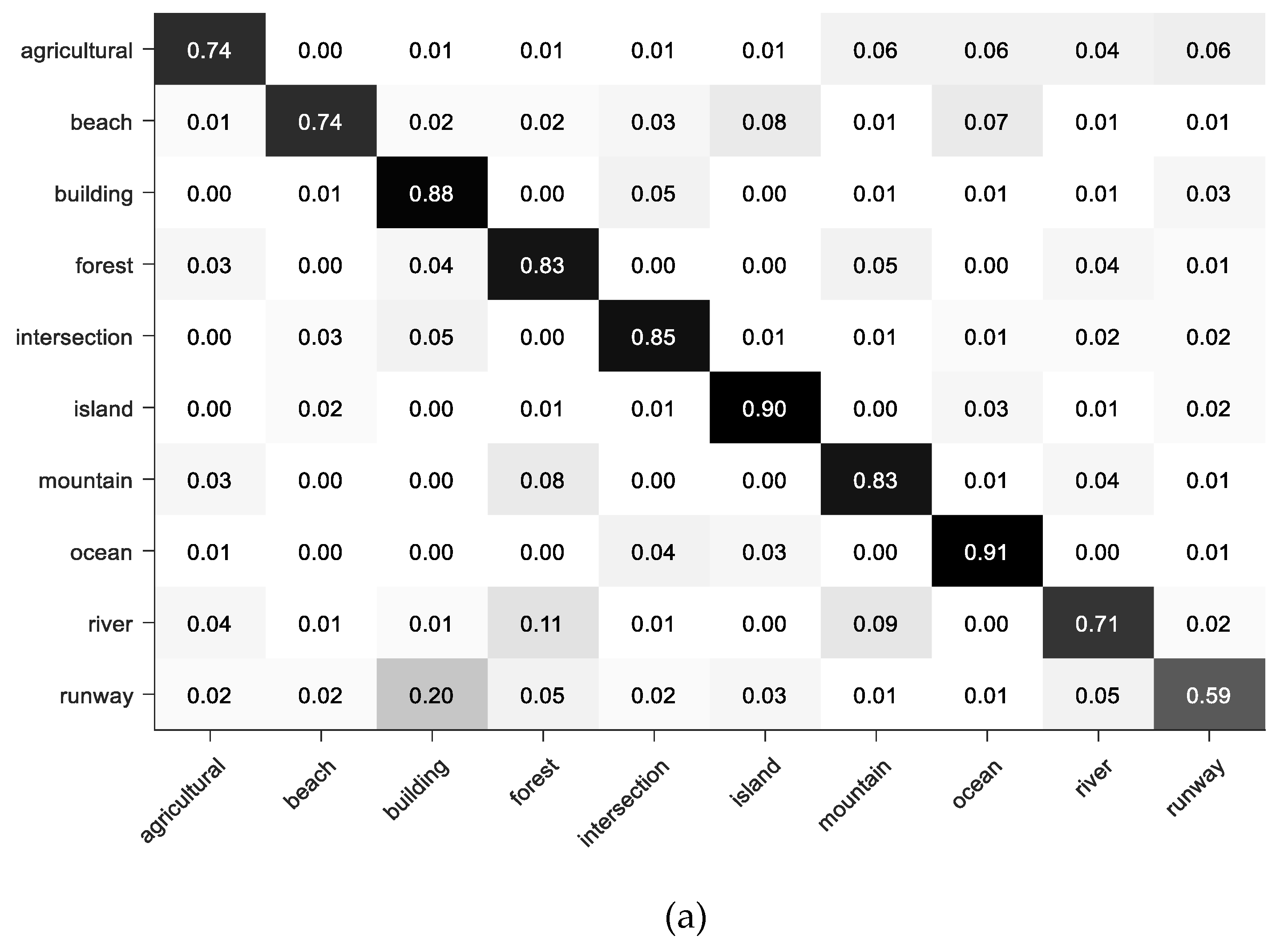
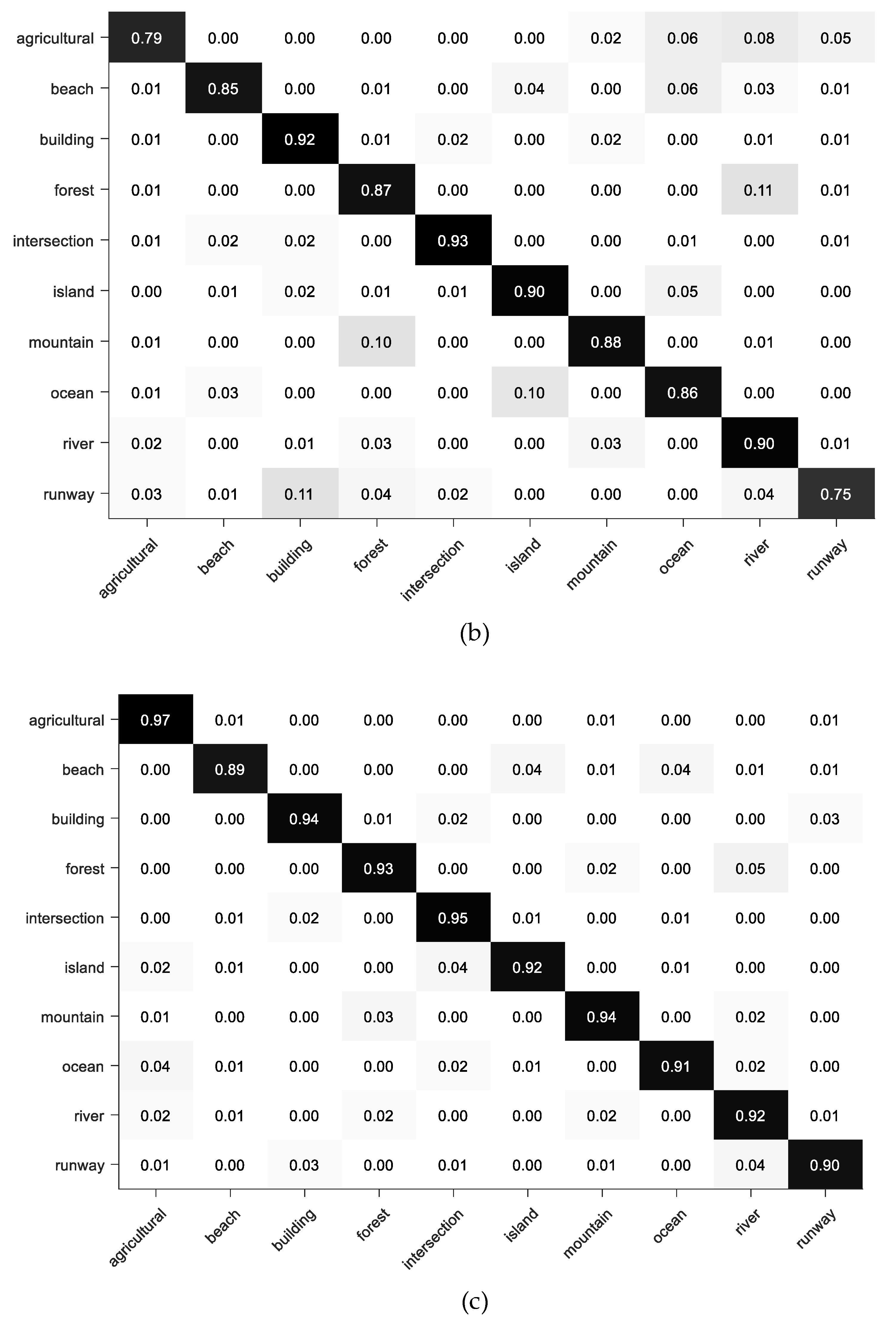
The confusion matrix reports the detailed classification results of each scene label; each column represents the predicted class, and each row represents the real class. As displayed in Figure 9, some scene categories such as agricultural, beach and runway cannot be effectively classified in the LLC+SIFT and VLAD+SIFT methods, but most categories are classified correctly and produce a classification accuracy higher than 90% in the proposed GCCH network; especially, the agricultural and intersection attain a classification accuracy higher than 95%. In addition, all of the scene classes get a higher score than the LLC+SIFT and VLAD+SIFT approaches. Therefore, the feature descriptors extracted by our proposed network are more discriminative than others.

4.3.5. The Ablation and Combined Experiments

We performed ablation and combined experiments to demonstrate the effectiveness of each module (parameterized LASC layer (PLASC), squeeze and excitation block (SE) and compact high-order generalized orderless pooling layer (CHG)). In this subsection, we truncate the conv5_3 layer of VGG-16 net as the standard convolution layer and make experiments under three different training-test ratios: 10%-90%, 20%-80% and 30%-70%.

We can observe that the VGG-16+CHG approach, which can be viewed as the first-order feature representation, achieves better performance than VGG-16 (fine tuning); meanwhile, LASC is locality-constrained affine subspace coding and constructs a dictionary consisting of an ensemble of linear subspaces attached to representative points, and PLASC contains the first and second-order feature representation. Therefore, vgg-16+PLASC is better than VGG-16 (fine tuning) and VGG-16+CHG. VGG-16+PLASC+SE learns the channel information of the parameterized LASC statistic representation by explicitly modelling the interdependencies between channels and acquires a higher score than VGG-16+PLASC. Similarly, VGG-16+PLASC+CHG can learn generalized compact high-order feature descriptors, which is more discriminative than VGG-16+PLASC and VGG-16+CHG. The GCCH network not only learns the channel information of the parameterized LASC statistic representation, but also acquires the high-order feature descriptors of channel-boosted parameterized LASC statistic representation; therefore, the proposed GCCH network acquires the highest score.

In addition, we introduce the computational complexity between the GCCH network and the ablation and combined networks in

Table 5. The ablation and combined experiments of the GCCH network.

Method	Time (Second)	TerraSAR-X Dataset
		10%	20%	30%
vgg-16(finetuning)	4.92	89.53	90.21	91.23
vgg-16+PLASC	1.77	91.14	92.58	92.91
vgg-16+CHG	1.53	90.51	92.12	92.38
vgg-16+PLASC+SE	3.58	91.42	92.60	93.12
vgg-16+PLASC+CHG	2.98	91.55	92.65	93.38
GCCH(Ours)	4.14	92.70	93.70	94.80

. The SAR remote sensing scene image resolution is $256*256$. The computational efficiency of each module is reported in detail. The proposed GCCH network truncates the conv5_3 layer of VGG-16 net, which does not contain the last three fully connected layers in VGG-16 net, and replaces them with PLASC, SE and CHG (they contain fewer parameters than the last three fully connected layers in VGG-16 net); therefore, the GCCH network runs faster than the VGG-16 (fine tuning) network.

5. Conclusions

The paper presents a novel effective network for SAR image scene classification, named the generalized compact channel-boosted high-order orderless pooling network (GCCH), which generates compact high-order and low-dimensional but highly discriminative feature descriptors. The proposed network learns the high-order of parameterized LASC (second-order feature coding style) by the kernelled outer product automatically, and the squeeze and excitation block is employed to learn the channel information of statistic feature representation by explicitly modelling the interdependencies between channels. All of the layers can be trained by back-propagation, and the parameters enable end-to-end optimization. Experimental results on the TerraSAR-X dataset demonstrate that the proposed GCCH network further improves the SAR scene classification performance, and performs better than other methods.

The full statistics of convolutional activations and higher-order feature coding style will be considered in future work. Furthermore, the high-order feature statistics information encoding on different network layers is worthy of study.

References

1. Ren, Z.L.; Hou, B.; Wen, Z.D.; Jiao, L.C. Patch-sorted deep feature learning for high resolution SAR image classification. IEEE J. Sel. Top. Appl. Earth Observ. Remote Sens. 2018, 11, 3113–3126. [Google Scholar] [CrossRef]
2. Esch, T.; Schenk, A.; Ullmann, T.; Thiel, M.; Roth, A.; Dech, S. Characterization of land cover types in terrasar-x images by combined analysis of speckle statistics and intensity information. IEEE Trans. Geosci. Remote Sens. 2011, 49, 1911–1925. [Google Scholar] [CrossRef]
3. Kwon, T.J.; Li, J.; Wong, A. Etvos: An enhanced total variation optimization segmentation approach for SAR sea-ice image segmentation. IEEE Trans. Geosci. Remote Sens. 2013, 51, 925–934. [Google Scholar] [CrossRef]
4. Yang, X.; Clausi, D. Evaluating SAR sea ice image segmentation using edge-preserving region-based MRFs. IEEE J. Sel. Top. Appl. Earth Observ. Remote Sens. 2012, 5, 1383–1393. [Google Scholar] [CrossRef]
5. Knuth, R.; Thiel, C.; Thiel, C.; Eckardt, R.; Richter, N.; Schmullius, C. Multisensor SAR analysis for forest monitoring in boreal and tropical forest environments. In Proceedings of the IEEE International Geoscience & Remote Sensing Symposium, Cape Town, South Africa, 12–17 July 2009. [Google Scholar]
6. Yang, S.; Wang, M.; Feng, Z.; Liu, Z.; Li, R. Deep sparse tensor filtering network for synthetic aperture radar images classification. IEEE T Neural Netw. Learn. Syst. 2018, 29, 3919–3924. [Google Scholar] [CrossRef]
7. Yang, S.; Wang, M.; Long, H.; Liu, Z. Sparse robust filters for scene classification of synthetic aperture radar (SAR) images. Neurocomputing 2006, 184, 91–98. [Google Scholar] [CrossRef]
8. Geng, J.; Wang, H.; Fan, J.; Ma, X. SAR image classification via deep recurrent encoding neural networks. IEEE Trans. Geosci. Remote Sens. 2017, 56, 2255–2269. [Google Scholar] [CrossRef]
9. Schmidhuber, J. Deep learning in neural networks: An overview. Neural Netw. 2015, 61, 85–117. [Google Scholar] [CrossRef] [PubMed] [Green Version]
10. Krizhevsky, A.; Sutskever, I.; Hinton, G.E. Imagenet classification with deep convolutional neural networks. Adv. Neural Inf. Process. Syst. 2012, 25, 1097–1105. [Google Scholar] [CrossRef]
11. Li, E.Z.; Xia, J.S.; Du, P.J.; Lin, C.; Samat, A. Integrating multilayer features of convolutional neural networks for remote sensing scene classification. IEEE Trans. Geosci. Remote Sens. 2017, 55, 5653–5665. [Google Scholar] [CrossRef]
12. He, N.J.; Fang, L.Y.; Li, S.T.; Plaza, A.; Plaza, J. Remote sensing scene classification using multilayer stacked covariance pooling. IEEE Trans. Geosci. Remote Sens. 2018, 56, 6899–6910. [Google Scholar] [CrossRef]
13. Matthew, D.Z.; Rob, F. Visualizing and understanding convolutional networks. In European Conference on Computer Vision; Springer: Berlin, Germany, 2014; pp. 818–833. [Google Scholar]
14. Gong, Y.C.; Wang, L.W.; Guo, R.Q.; Lazebnik, S. Multi-scale orderless pooling of deep convolutional activation features. In European Conference on Computer Vision; Springer: Berlin, Germany, 2014; pp. 392–407. [Google Scholar]
15. Silva, F.B.; Werneck, R.D.O.; Goldenstein, S.; Tabbone, S.A. Graph-based bag-of-words for classification. Pattern Recogn. 2017, 74, 266–285. [Google Scholar] [CrossRef]
16. Xie, X.M.; Zhang, Y.Z.; Wu, J.J.; Shi, G.M.; Dong, W.S. Bag-of-words feature representation for blind image quality assessment with local quantized pattern. Neurocomputing 2017, 266, 176–187. [Google Scholar] [CrossRef]
17. Sun, H.; Sun, X.; Wang, H.; Li, Y.; Li, X. Automatic target detection in high-resolution remote sensing images using spatial sparse coding bag-of-words model. IEEE Geosci. Remote Sens. Lett. 2012, 9, 109–113. [Google Scholar] [CrossRef]
18. Li, Y.; Liu, L.Q.; Shen, C.H.; Hengel, A.V.D. Mining mid-level visual patterns with deep CNN activations. Int. J. Comput. Vis. 2015, 121, 971–980. [Google Scholar] [CrossRef]
19. Sivic, J. A text retrieval approach to object matching in videos. In Proceedings of the Ninth IEEE International Conference on Computer Vision, Nice, France, 13–16 October 2003. [Google Scholar]
20. Lazebnik, S. Beyond bags of features: Spatial pyramid matching for recognizing natural scene categories. In Proceedings of the IEEE Computer Society Conference on Computer Vision and Pattern Recognition, New York, NY, USA, 17–22 June 2006. [Google Scholar]
21. Sheng, G.F.; Yang, W.; Xu, T.; Sun, H. High-resolution satellite scene classification using a sparse coding based multiple feature combination. Int. J. Remote Sens. 2012, 33, 2395–2412. [Google Scholar] [CrossRef]
22. Wang, J.; Yang, J.; Kai, Y.; Lv, F.; Huang, T.; Gong, Y. Locality-constrained Linear Coding for image classification. In Proceedings of the IEEE Computer Society Conference on Computer Vision and Pattern Recognition, San Francisco, CA, USA, 13–18 June 2010. [Google Scholar]
23. Zhou, X.; Yu, K.; Zhang, T.; Huang, T.S. Image classification using super-vector coding of local image descriptors. In European Conference on Computer Vision; Springer: Berlin, Germany, 2010; Volume 6315, pp. 141–154. [Google Scholar]
24. Sánchez, J.; Perronnin, F.; Mensink, T.; Verbeek, J. Image classification with the fisher vector: Theory and practice. Int. J. Comput. Vis. 2013, 105, 222–245. [Google Scholar] [CrossRef]
25. Li, P.; Lu, X.; Wang, Q. From dictionary of visual words to subspaces: Locality-constrained affine subspace coding. In Proceedings of the IEEE Conference on Computer Vision and Pattern Recognition, Boston, MA, USA, 7–12 June 2015. [Google Scholar]
26. Zhu, Q.; Zhong, Y.; Zhao, B.; Xia, G.S.; Zhang, L. Bag-of-visual-words scene classifier with local and global features for high spatial resolution remote sensing imagery. IEEE Geosci. Remote Sens. Lett. 2016, 13, 747–751. [Google Scholar] [CrossRef]
27. Hu, F.; Xia, G.S.; Hu, J.W.; Zhang, L.P. Transferring deep Convolutional Neural Networks for the scene classification of high-resolution remote sensing imagery. Remote Sens. 2015, 7, 14680–14707. [Google Scholar] [CrossRef]
28. Qi, K.; Wu, H.; Shen, C.; Gong, J. Land-use scene classification in high-resolution remote sensing images using improved correlatons. IEEE Geosci. Remote Sens. Lett. 2015, 12, 2403–2407. [Google Scholar]
29. Bian, X.; Chen, C.; Tian, L.; Du, Q. Fusing local and global features for high-resolution scene classification. IEEE J. Sel. Top. Appl. Earth Observ. Remote Sens. 2017, 10, 2889–2901. [Google Scholar] [CrossRef]
30. Mekhalfi, M.L.; Melgani, F.; Bazi, Y.; Alajian, N. Land-use classification with compressive sensing multifeature fusion. IEEE Geosci. Remote Sens. Lett. 2015, 12, 2155–2159. [Google Scholar] [CrossRef]
31. Cheng, G.; Li, Z.; Yao, X.; Guo, L.; Wei, Z. Remote sensing image scene classification using bag of convolutional features. IEEE Geosci. Remote Sens. Lett. 2017, 14, 1735–1739. [Google Scholar] [CrossRef]
32. Yuan, B.; Li, S.; Li, N. Multiscale deep features learning for land-use scene recognition. J. Appl. Remote Sens. 2018, 12, 015010. [Google Scholar] [CrossRef]
33. Banerjee, B.; Chaudhuri, S. Scene recognition from optical remote sensing images using mid-level deep feature mining. IEEE Geosci. Remote Sens. Lett. 2018, 15, 1080–1084. [Google Scholar] [CrossRef]
34. Yang, Y.; Newsam, S. Bag-of-visual-words and spatial extensions for land-use classification. In Proceedings of the 18th Sigspatial International Conference on Advances in Geographic Information Systems, New York, NY, USA, 2–5 November 2010. [Google Scholar]
35. Fan, J.; Chen, T.; Lu, S. Unsupervised feature learning for land-use scene recognition. IEEE Trans. Geosci. Remote Sens. 2017, 50, 2250–2261. [Google Scholar] [CrossRef]
36. Dalal, N.; Triggs, B. Histograms of oriented gradients for human detection. In Proceedings of the Computer Society Conference on Computer Vision and Pattern Recognition, San Diego, CA, USA, 20–25 June 2005. [Google Scholar]
37. Arandjelovic, R.; Gronat, P.; Torii, A.; Pajdla, T.; Sivic, J. Netvlad: CNN architecture for weakly supervised place recognition. IEEE Trans. Pattern Anal. Mach. Intell. 2018, 40, 1437–1451. [Google Scholar] [CrossRef]
38. Jegou, H.; Douze, M.; Schmid, C.; Perez, P. Aggregating local descriptors into a compact image representation. In Proceedings of the IEEE Computer Society Conference on Computer Vision and Pattern Recognition, San Francisco, CA, USA, 13–18 June 2010. [Google Scholar]
39. Chen, B.; Li, J.; Wei, G.; Ma, B. A novel localized and second order feature coding network for image recognition. Pattern Recogn. 2018, 76, 339–348. [Google Scholar] [CrossRef]
40. Ni, K.; Wang, P.; Wu, Y.Q. High-order generalized orderless pooling networks for synthetic-aperture radar scene classification. Available online: http://openaccess.thecvf.com/content_cvpr_2018/html/Hu_Squeeze-and-Excitation_Networks_CVPR_2018_paper.html (accessed on 23 April 2019).
41. Hu, J.; Shen, L.; Albanie, S.; Sun, G.; Wu, E. Squeeze-and-excitation networks. Available online: https://ieeexplore.ieee.org/abstract/document/8695749 (accessed on 29 April 2019).
42. Nogueira, K.; Penatti, O.A.B.; Santos, J.A.D. Towards better exploiting Convolutional Neural Networks for remote sensing scene classification. Pattern Recogn. 2017, 61, 539–556. [Google Scholar] [CrossRef]
43. Lin, R.; Xiao, J.; Fan, J. Nextvlad: An efficient neural network to aggregate frame-level features for large-scale video classification. In Proceedings of the Workshop on Statistical Learning in Computer Vision ECCV, Munuch, Germany, 8–14 September 2018. pp. 206–218.
44. Lin, T.Y.; Roychowdhury, A.; Maji, S. Bilinear cnn models for fine-grained visual recognition. In Proceedings of the IEEE International Conference on Computer Vision, Santiago, Chile, 7–13 December 2015. pp. 1449–1457.
45. Kong, S.; Fowlkes, C. Low-rank bilinear pooling for fine-grained classification. In Proceedings of the IEEE Conference on Computer Vision and Pattern Recognition, Honolulu, HI, USA, 21–26 July 2017. [Google Scholar]
46. Gao, Y.; Beijbom, O.; Zhang, N.; Darrell, T. Compact bilinear pooling. In Proceedings of the IEEE Conference on Computer Vision and Pattern Recognition, Las, Vegas, NV, USA, 27–30 June 2016. pp. 317–326.
47. He, K.; Zhang, X.; Ren, S.; Sun, J. Deep residual learning for image recognition. In Proceedings of the IEEE Conference on Computer Vision and Pattern Recognition, Las, Vegas, NV, USA, 27–30 June 2016. pp. 770–778.
48. Zegedy, C.; Liu, W.; Jia, Y.; Sermanet, P.; Reed, S.; Anguelov, D.; Erhan, D.; Vanhoucke, V.; Rabinovich, A. Going deeper with convolutions. In Proceedings of the IEEE Conference on Computer Vision and Pattern Recognition, Boston, MA, USA, 7–12 June 2015. pp. 1–9.
49. Sun, Y.; Liu, Z.P.; Todorovic, S.; Li, J. Adaptive boosting for SAR automatic target recognition. IEEE T Aero Elec Sys. 2005, 43, 112–125. [Google Scholar] [CrossRef]
50. Lowe, D.G. Distinctive image features from scale-invariant keypoints. Int. J. Comput. Vis. 2004, 60, 91–110. [Google Scholar] [CrossRef]
Figure 1. The synthetic aperture radar (SAR) scene images in the same class. (a) and (b) are the agricultural images, (c) and (d) are the building images.
Remotesensing 11 01079 g001
Figure 2. The overall framework of the generalized compact channel-boosted high-order orderless pooling (GCCH) network. The proposed GCCH network includes the standard convolution layers, second-order generalized layer (parameterized locality constrained affine subspace coding (LASC) layer), squeeze and excitation block, and the compact high-order generalized orderless pooling layer. The black arrow represents the forward operation of the proposed network; all of the parameters can be updated by back-propagation in the GCCH network.
Remotesensing 11 01079 g002
Figure 3. The illustration of the traditional LASC method. The LASC features are extracted by hand crafting, such as the histogram of oriented gradient (HOG) [36], and the dictionary of LASC is an ensemble of low-dimensional linear subspaces attached to the affine subspaces.
Remotesensing 11 01079 g003
Figure 4. The network architecture of the parameterized LASC layer. The input of the parameterized LASC layer is the standard convolution layer in the convolutional neural network (CNN), which is a D dimensional feature vector. Both the dimensionality of the first-order and second-order LASC statistical information are K × S . Finally, we cascade them.
Remotesensing 11 01079 g004
Figure 5. The schematic of squeeze and excitation block, including the squeeze operation and excitation operation.
Remotesensing 11 01079 g005
Figure 6. Example images from the TerraSAR-X dataset: (a) agricultural; (b) beach; (c) building; (d) forest; (e) intersection; (f) island; (g) mountain; (h) ocean; (i) river; (j) runway.
Remotesensing 11 01079 g006
Figure 7. Influence of projected dimensions in the GCCH network.
Remotesensing 11 01079 g007
Figure 8. Comparison between the GCCH network and other state-of-the art methods on the TerraSAR-X dataset. (a) 10%. (b) 20%. (c) 30%.
Remotesensing 11 01079 g008aRemotesensing 11 01079 g008b
Figure 9. Confusion matrices of the TerraSAR-X dataset under the training ratio of 10% using the following methods: (a) LLC+SIFT. (b) VLAD+SIFT. (c) GCCH (ours).
Remotesensing 11 01079 g009aRemotesensing 11 01079 g009b