A Spectral Unmixing Method by Maximum Margin Criterion and Derivative Weights to Address Spectral Variability in Hyperspectral Imagery

Abstract

Limited to the low spatial resolution of the hyperspectral imaging sensor, mixed pixels are inevitable in hyperspectral images. Therefore, to obtain the endmembers and corresponding fractions in mixed pixels, hyperspectral unmixing becomes a hot spot in the field of remote sensing. Endmember spectral variability (ESV), which is common in hyperspectral images, affects spectral unmixing accuracy. This paper proposes a spectral unmixing method based on maximum margin criterion and derivative weights (MDWSU) to reduce the effect of ESV on spectral unmixing. Firstly, in the MDWSU model, an effective and fast algorithm is employed for establishing the endmember spectral library. Then a spectral weighting matrix based on the maximum margin criterion is constructed based on the endmember spectral library. Besides, derivative analysis and local neighborhood weights are merged into local neighborhood derivative weights, which act as a regularization term to penalize different abundance vectors. Local neighborhood derivative weights and spectral weighting matrix are proved to reduce the effect of ESV. Real hyperspectral data experiments show that the MDWSU model can obtain more accurate endmembers and abundance estimation. In addition, the experimental results, including the spectral angle distance and the root mean square error, prove the superiority of the MDWSU model over the previous methods.

1. Introduction

Hyperspectral imaging is the multi-dimensional information acquisition technology combining imaging technology and spectroscopy technology. It simultaneously detects two-dimensional geometric spatial information and one-dimensional spectral information of the scene, and acquires continuous, narrow-band image data with high spectral resolution. Limited to the low spatial resolution of the hyperspectral imaging sensors, in spite of utilizing super-resolution techniques [1] the area corresponding to a single pixel in the hyperspectral image usually covers disparate substances. The spectral information of the pixel is actually a mixture of spectra of disparate substances, and such pixels are called mixed pixels. If one pixel contains only one substance, the pixel is a pure pixel. Mixed pixels arise for one of two reasons: first, some substance may become the major substance in the mixed pixels when the spatial resolution of the image is lower; second, mixed pixels appear when distinct materials are combined into a homogeneous mixture [2]. Spectral unmixing, which decomposes a mixed pixel into a collection of constituent spectra, or endmembers, and their corresponding fractional abundances [2,3], can obtain sub-pixel level information and improve the accuracy of substance recognition. Therefore, spectral unmixing makes a lot of sense and has become a research hotspot in recent years.

Spectral unmixing involves two main aspects, namely endmember extraction and abundance estimation. In most traditional endmember extraction algorithms, it is assumed that the spectral characteristics of different endmembers have differences between categories and spatiotemporal stability, that is, different endmembers have absolutely different spectral characteristic curves and spectral curves of the same endmembers are not affected by external factors. However, affected by factors such as sensors, the atmosphere, and the surrounding environment, endmember spectral variability (ESV) is an inevitable phenomenon in hyperspectral images [4,5,6,7]. ESV will greatly affect the accuracy of spectral unmixing [4,7]. In this paper, we focus on reducing the effect of endmember spectral variability on spectral unmixing. Changes in the distribution of material properties, differences in illumination conditions, changes in atmospheric conditions, and changes in natural factors such as time and space can cause spectral variability of endmembers [5,8]. The change in illumination radiation is caused by varying degrees of shadow and bright areas due to changes in the surface of the material. The strong absorption and scattering properties of the atmosphere affect the measurement of the spectrum. Due to changes in the intrinsic parameters of the material (e.g., the concentration of suspended solids in water), the inherent change in the material also changes the reflectivity of the material [6,9]. Endmember spectral variability includes two categories, namely intra-class variability and inter-class variability [5,10]. Spectral variation within one endmember class is called intra-class variability (e.g., the spectra of intra-tree can vary from tree to tree within a given tree species) and spectral variation between endmember classes (e.g., crops and weeds) is called inter-class variability. Especially, the accuracy of abundance estimation linearly decreases in the presence of intra-class variability. On one hand, the higher the intra-class variability, the higher the probability that the actual spectrum of the endmember in the single pixel deviates from the fixed endmember. On the other hand, the high similarity between the endmembers leads to a high correlation between the endmember spectra, which causes a decrease in the accuracy of the abundance estimation [5]. Therefore, reducing the effect of ESV is an effective approach to improve the spectral unmixing accuracy.

To overcome the effect of endmember spectral variability, different algorithms have been proposed. Various algorithms focus on narrowing intra-class variability and expanding inter-class variability to a certain extent to improve the abundance estimation precision. Somers et al. classify existing algorithms for coping with ESV into five categories: iterative mixture analysis, spectral feature selection, spectral weighting bands, spectral transformation, and spectral models [5]. (1) To accomplish the iterative mixture analysis algorithms, an endmember combination candidate library consisting of all possible endmember combinations is needed to define firstly. Then, for each mixed pixel, the optimal endmember combination suitable for the pixel is selected from the endmember combination candidate library by the loop iteration method. Multiple endmember spectral mixture analysis (MESMA) [11] is one of the most widely used algorithms [12,13]. In the MEMSA algorithm, each endmember class is represented by a set of intra-class endmember spectra, all endmember combinations variable in category and quantity for each pixel are exhausted, and the optimal endmember combination with the minimum reconstruction error between the pixel reconstruction value and the real pixel value as the criterion is selected to unmix the corresponding pixel. Although such an algorithm can effectively cope with variability, it has the disadvantage of frequent preselection of endmember sets. In addition, the premise of the MESMA algorithm is the availability of a spectral library containing all representative instances of the whole endmembers in the hyperspectral scene. Such spectral libraries are commonly modeled by filed measurements. In an operational setting, these libraries of field measurements may not be available, thus limitations in the operational applicability of MESMA are introduced [14]. Therefore, an automatic extraction of image-based endmember bundles and a new extended linear mixture model are proposed to address ESV [14,15]. (2) Another existing algorithm includes spectral feature selection [16]. A specific index is used as the evaluation index, the index values of each band are sorted, and the spectral feature combinations that minimize the intra-class variability and maximize inter-class variability are selected. Commonly used spectral feature selection algorithms include mutual information (MI) [17], instability index (ISI) [18], and so on. Although such an algorithm can effectively avoid the excessive calculation, some information will be lost during the spectral feature selection process. (3) Another existing algorithm includes spectral weighting bands. On the basis of the equal weight of each band participation in spectral unmixing, the algorithm gives greater weight to the bands that have less correlation with intra-class differences and greater correlation with inter-class differences. Such algorithms reduce the effect of endmember spectral variability and perform better than traditional unweighted algorithms [19]. (4) Spectral transformation is used to convert the original hyperspectral data into new spectral features with smaller intra-class differences and larger inter-class differences for spectral unmixing. Common spectral transformation methods include principle component analysis (PCA) [20], wavelet transform [21], derivative spectral unmixing [22], and normalized spectral mixture analysis [23]. The spectral transformation process reduces data redundancy. (5) Based on the theory of various radioactive transfer models, the spectral modeling algorithms construct the corresponding spectral library according to the specific environment and climate of the research area. But the accurate construction of the spectral model requires a certain prior knowledge. Analyzing and comparing all of the above methods, a method combining spectral transformation and spectral weighting bands is proposed to reduce the influence of ESV, thereby improving spectral unmixing precision.

A spectral unmixing method based on maximum margin criterion and derivative weights (MDWSU) is proposed in the paper to address ESV in hyperspectral imagery. To cope with endmember spectral variability, the endmember spectral library firstly needs to be acquired. Zou et al. select typical endmembers from the image by visual interpretation method or perform field acquisition experiments to obtain endmember spectra [24]. However, the above-mentioned methods are labor intensive and the established endmember spectral library is not suitable for all scenarios. Jin et al. [25] select a certain number of pure pixels as the training samples of each endmember through the purity pixel index (PPI) [26] algorithm, but the PPI algorithm randomly generates the projection vector, which cannot guarantee the accuracy of obtaining the endmember. Inspired by the literature [25], we focus on building endmember spectral library from images automatically. This paper tends to explore an effective method to acquire endmember spectral libraries adapted for different scenarios. On the basis of the endmember spectral library, a weighting matrix assigned to different band weights is constructed. The maximum margin criterion (MMC) [27] will be introduced into the construction of the spectral weighting matrix. MMC is applied to find the linear transform that maximizes inter-class differences, while minimizing intra-class differences. Meanwhile, derivative weights in local neighborhood are designed to improve spectral unmixing accuracy. Different from the weights designed in weighted nonnegative matrix factorization [28], the paper uses the first derivative of the spectrum to construct weights. Utilization of the available spectral information is a challenge in hyperspectral remote sensing analysis. The available spectral information involves the spectral magnitude and spectral shape. Due to the changes in the atmosphere and topography, the spectral magnitude of the same endmember is more affected than the spectral shape of the same endmember. The computation of derivative spectra is sensitive to the spectral shape rather than the magnitude of spectra and can precisely model changes in the shape of original spectra [22]. At last, the proposed method is experimented on synthetic and real hyperspectral data to verify its validity.

The rest of the paper is organized as follows. The second part presents the proposed theoretical methodology. The third part presents the experimental data acquisition process. The fourth part shows the experimental results and analysis. The fifth part provides discussion about the proposed method, experimental results, and suggestions for the future research. Finally, the sixth part summarizes the paper.

2. Theoretical Methodology

Linear mixture model or nonlinear mixture model are common models when modeling mixed pixels. Generally speaking, the linear mixture model is regarded as mixtures for which the pixel components are homogeneous surfaces in spatially segregated patterns. On the contrary, the nonlinear mixture model takes the intimate association or interaction with more than one component into account [24]. Most algorithms prove that the linear mixture model is an effective model which can meet the accuracy requirements. The linear model conforms to the formation mechanism of hyperspectral image. In this paper, the proposed algorithm model will be introduced based on the linear mixture model. Figure 1 shows the schematic overview of the proposed method.

2.1. Linear Mixture Model

The linear mixture model is established under the following three assumptions. Firstly, spectral signal of the pixel is a linear combination of spectra of a finite number of endmembers with their corresponding abundance fractions. Secondly, the land covers are regarded as homogeneous surfaces. Thirdly, the radiation reflection of neighboring pixels within each instantaneous field of view (IFOV) of the imaging sensor will not interact [29,30,31].

For the l-band hyperspectral image containing n pixels with m endmembers, the linear mixture model is expressed in Equation (1).

$$\mathit{X}=\mathit{G}\mathit{A}+\mathit{\epsilon }$$

(1)

where $\mathit{X}=\left[{\mathit{x}}_1,\dots ,{\mathit{x}}_n\right]\in {\mathbb{R}}^{l\times n}$ represents the hyperspectral image (${\mathit{x}}_i$ represents the i^th pixel regarded as l-band spectral vector, l denotes the number of the total bands, n denotes the number of the total pixels); $\mathit{G}=\left[{\mathit{g}}_1,\dots ,{\mathit{g}}_m\right]\in {\mathbb{R}}^{l\times m}$ represents the endmember matrix (${\mathit{g}}_i$ represents the i^th endmember signature); $\mathit{A}=\left[{\mathit{a}}_1,\dots ,{\mathit{a}}_n\right]\in {\mathbb{R}}^{m\times n}$ denotes abundance fractions; $\mathit{\epsilon }$ denotes model error.

${\mathit{A}}_{ij}$ denotes the coverage percentage of the area occupied by the i^th endmember in the j^th pixel. Under the guidance of the linear mixture model assumption, ${\mathit{A}}_{ij}$ is non-negative and the sum of each column of $\mathit{A}$ is unity. ${\mathit{A}}_{ij}$ can be expressed in Equation (2).

$$\begin{array}{c}{\mathit{A}}_{ij}\ge 0,\forall i,j\\ {\displaystyle {\displaystyle \sum }_{i=1}^m}{\mathit{A}}_{ij}=1,j=1,2,\dots ,n \end{array}$$

(2)

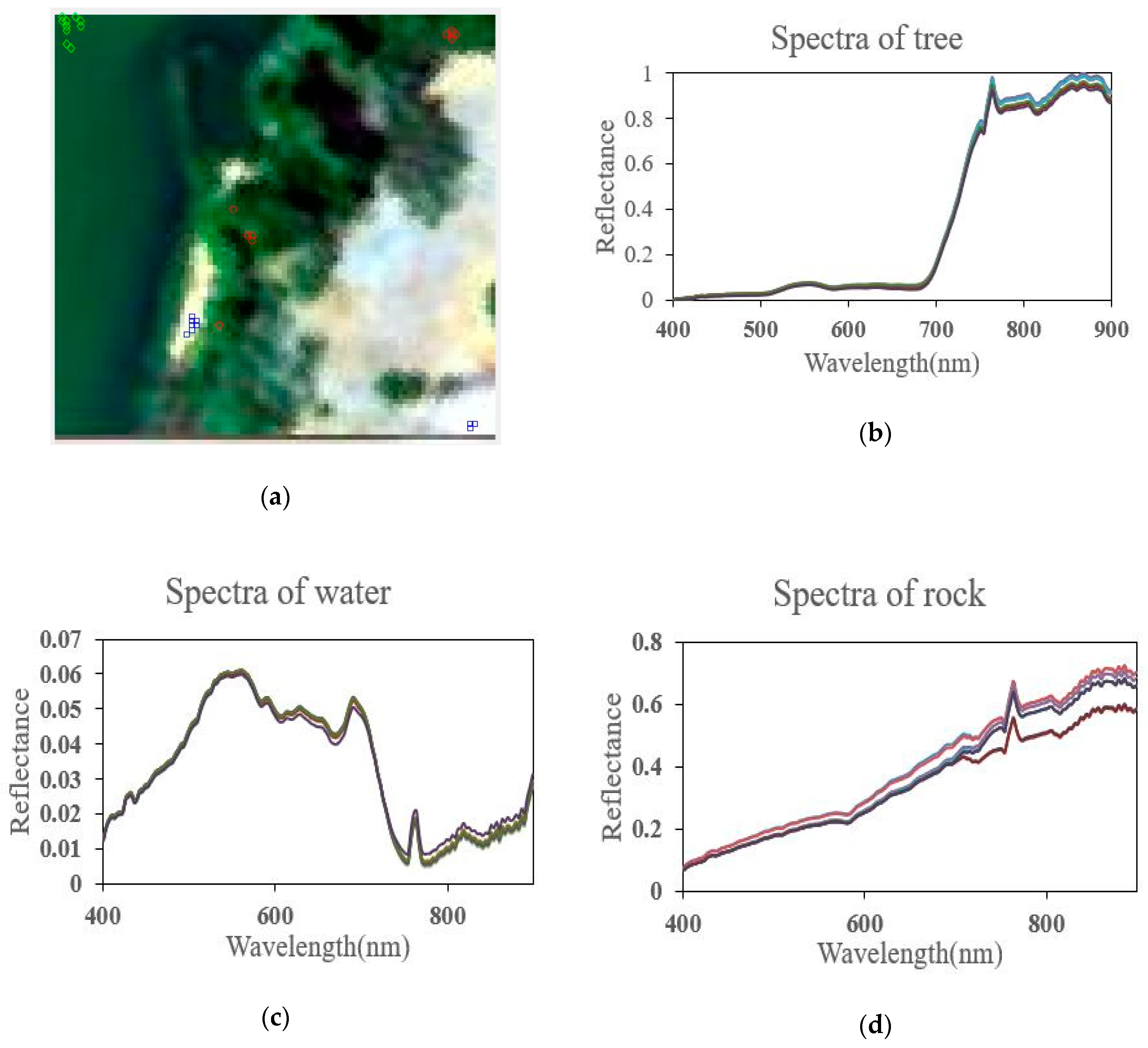
2.2. Modeling Endmember Spectral Library

In order to avoid the subjective misjudgment of the visual interpretation method and the human burden caused by the field experiment, the paper will extract the optimal endmember spectral library from the hyperspectral image. Based on the endmember spectral library, a spectral weighting matrix is constructed.

All of the pixels in the hyperspectral image can form a simplex with the endmembers as the vertices. Vertex component analysis (VCA) algorithm uses the orthogonal projection method to find the vertices of simplex as endmembers [32]. Several vertices of the simplex can be expanded into the subspace, and the maximum point of projection length of the simplex in the orthogonal complement space of the subspace must be the vertices of the simplex. Therefore, at each cycle, the VCA algorithm finds a projection matrix that is orthogonal to the known endmember set, and projects all the pixels onto the matrix, and records the pixel with the largest projection length as the new endmember, then starts the next iteration until all the endmembers are found. Assuming that k endmembers marked as ${\left\{{\mathit{g}}_i\right\}}_{\mathit{i}=\mathbf{1}}^{\mathit{k}}$ have been extracted, the k endmembers can be expanded into the k-dimensional subspace ${\mathit{G}}_k$. The base matrix of the orthogonal complement space ${\mathit{G}}_k^{\perp }$ of ${\mathit{G}}_k$ is as follows:

$${\mathit{G}}_k^{\perp }={\mathit{I}}_k-{\mathit{G}}_k{\left({\mathit{G}}_k^T{\mathit{G}}_k\right)}^{-1}{\mathit{G}}_k^T$$

(3)

where ${\mathit{I}}_k$ represents the k-dimensional unit matrix, (.)^T represents transpose of the matrix, ${\mathit{G}}_k$ represents $\left[{\mathit{g}}_1,\dots ,{\mathit{g}}_k\right]$.

The projection matrix ${\mathit{\omega }}_k^{\perp }$ of the VCA algorithm is shown in Equation (4).

$${\mathit{\omega }}_k^{\perp }=\frac{{\mathit{G}}_k^{\perp }\mathit{\xi }}{\Vert {\mathit{G}k\perp \mathit{\xi }\Vert }_{\mathbf{2}}}$$

(4)

where $\mathit{\xi }$ is independent and identically distributed zero-mean Gaussian vector, $\mathit{\xi }\sim N\left(\mathbf{0},{\mathit{I}}_k\right)$.

The VCA algorithm projects the pixel x_i according to the Equation (5). The projection results in Equation (5) form a new dataset ${\left\{{\widehat{\mathit{x}}}_i\right\}}_{\mathit{i}=\mathbf{1}}^{\mathit{n}}$, in which the largest value can be regarded as a new endmember.

$${\widehat{\mathit{x}}}_i={\mathit{\omega }}_k^{\perp }{\mathit{x}}_i$$

(5)

The above analysis is the basic principle of VCA extraction endmember algorithm. According to the above analysis, pure pixels located at the vertices of the simplex are treated as endmembers. Using a simplex to approximate the hyperspectral data, the pixels near the vertices of the simplex are of high purity. Pixels with high purity are viewed as endmember training samples. Inspired by the principle of VCA extraction endmember algorithm, the orthogonal projection method can be applied to find the pixels near or at the vertices of the simplex as the candidates of the endmember spectral library. In the IEA algorithm, Neville et al. select the average of several pure pixels as the optimal endmember spectrum, which can improve the spectral unmixing accuracy and reduce the noise and error [33].

Under the guidance of the above analysis, the algorithm of modeling endmember spectral library in the paper is described below.

Step (1)

Determine that the class number of endmembers is m and the number of spectra contained in each endmember is t.

Step (2)

Initialize the endmember matrix $\mathit{G}=\left[{\mathit{g}}_1,\dots ,{\mathit{g}}_m\right]$ by VCA algorithm.

Step (3)

For each endmember k = 1, …, m, the algorithm constructs the new endmember set that removes the k^th endmember ${\mathit{g}}_{\mathit{K}}$. The new endmember set is marked as ${\tilde{\mathit{G}}}_k=\left[{\mathit{g}}_1,\dots ,{\mathit{g}}_{k-1},{\mathit{g}}_{k+1},\dots ,{\mathit{g}}_m\right]$. According to the Equations (3)–(5), the algorithm generates the projection matrix ${\mathit{\omega }}_k^{\perp }$ orthogonal to the endmembers set ${\tilde{\mathit{G}}}_k$, projects all the pixels of the hyperspectral image onto the matrix, and records the pixels of the first t maximum projection length as the spectrum library $C_k$ of the k^th endmember. The average of the t pixels is regarded as the improved spectrum ${\overline{\mathit{g}}}_k$ of the k^th endmember. The k^th endmember ${\mathit{g}}_k$ is replaced with ${\overline{\mathit{g}}}_k$ in the initial endmember matrix $\mathit{G}$.

Step (4)

Repeat step (3) until the spectral library and the improved spectra of all the endmembers are found.

Then the above-mentioned algorithm is applied to the Samson hyperspectral dataset in Figure 2 to construct endmember spectrum library. The hyperspectral dataset in Figure 2 consists of 95 × 95 pixels. The Samson hyperspectral dataset covering spectral wavelength between 400 nm and 900 nm with spectral resolution of 3.2 nm can be available online [34]. WeoGeo provides this hyperspectral dataset owned by Oregon State University. The hyperspectral dataset was obtained by the SAMSON instrument which is a push-broom, visible to near IR, hyperspectral imaging sensor. Figure 2 shows the position of endmember candidates of endmember spectral library. In Figure 2, red circles represent tree, green diamonds represent water, and blue squares represent rock.

2.3. Spectral Weighting Matrix

The most traditional algorithms assign equal weight to different bands which are assumed to have uniform effects. However, it may not be necessarily true since every band is not necessarily equally significant. The experimental results have already shown the weighting spectral unmixing methods outperform the traditional unweighted unmixing methods [35]. Therefore, spectral weighting matrix K defined in the Equation (6) is introduced into the proposed method. It is obvious that K is a positive-definite and symmetric matrix. When K is chosen to be the identity matrix, it means to assign the equal weight to different bands.

$$\mathit{K}=diag({\displaystyle \sum }_{k=1}^m{\displaystyle \sum }_{\mathit{x}\in C_k}^{}\left(\mathit{x}-{\mathit{x}}_k^I\right){\left(\mathit{x}-{\mathit{x}}_k^I\right)}^T)$$

(6)

where K is the diagonal matrix of the intra-class scatter matrix, $\mathit{x}\in {\left\{C_k\right\}}_{K=1}^m$ are $m\times t$ training sample spectral vectors given by the algorithm of modeling endmember spectral library, $C_k$ denotes the training sample vectors of the endmember spectral library of the k^th class, and ${\mathit{x}}_k^I$ is the intra-class furthest neighbor of the sample $\mathit{x}\in C_k$. ${\mathit{x}}_k^I$ is defined in the Equation (7).

$${\mathit{x}}_k^I=\left\{{\mathit{x}}_k^I\in C_k|\Vert {\mathit{x}}_k^I-\mathit{x}\Vert >\Vert \mathit{z}-\mathit{x}\Vert ,\forall \mathit{z}\in C_k\right\}$$

(7)

Inspired by maximum margin criterion (MMC), spectral weighting matrix K in the proposed method tries to make the samples in the same class as compact as possible, which is conductive to reduce the spectral variability of the same endmember. Figure 3 provides an explanation of MMC. In Figure 3, the red circle assigned to be center point has six neighbors. The red circle and the black circles belong to the same class. The red circle and the yellow rectangle and triangle do not belong to the same class. After MMC, the samples in the same class become more compact.

In general, the model in Equation (1) can be interpreted as least squares error (LSE) problem [35].

$${\left(\mathit{x}-\mathit{G}\mathit{a}\right)}^{\mathit{T}}\left(\mathit{x}-\mathit{G}\mathit{a}\right)$$

(8)

The model in (1) is assumed to different bands have uniform effects on LSE. Then we introduce the weighting matrix K into Equation (8) so that LSE can be turned into a weighted LSE approach, which can be described in the Equation (9).

$$\begin{gathered} {\left(\mathit{x}-\mathit{G}\mathit{a}\right)}^{\mathit{T}}{\mathit{K}}^{-\mathbf{1}}\left(\mathit{x}-\mathit{G}\mathit{a}\right)= {\left(\mathit{x}-\mathit{G}\mathit{a}\right)}^{\mathit{T}}{\mathit{K}}^{-\mathbf{1}/\mathbf{2}}{\mathit{K}}^{-\mathbf{1}/\mathbf{2}}\left(\mathit{x}-\mathit{G}\mathit{a}\right) \\ ={\left({\mathit{K}}^{-\frac{\mathbf{1}}{\mathbf{2}}}\mathit{x}-{\mathit{K}}^{-\frac{\mathbf{1}}{\mathbf{2}}}\mathit{G}\mathit{a}\right)}^{\mathit{T}}\left({\mathit{K}}^{-\frac{\mathbf{1}}{\mathbf{2}}}\mathit{x}-{\mathit{K}}^{-\frac{\mathbf{1}}{\mathbf{2}}}\mathit{G}\mathit{a}\right)={(\stackrel{=}{\mathit{x}}-\stackrel{=}{\mathit{G}}\mathit{a})}^{\mathit{T}}(\stackrel{=}{\mathit{X}}-\stackrel{=}{\mathit{G}}\mathit{a}) \end{gathered}$$

(9)

A weighted LSE approach assign different weights to different bands, so that endmember matrix $\mathit{G}$ can be transformed into $\stackrel{=}{\mathit{G}}$ and hyperspectral image $\mathit{X}$ can be transformed into $\stackrel{=}{\mathit{X}}$.

$$\begin{gathered} \stackrel{=}{\mathit{X}}=\left[{\stackrel{=}{\mathit{x}}}_1,\dots ,{\stackrel{=}{\mathit{x}}}_n\right]\in {\mathbb{R}}^{l\times n}={\mathit{K}}^{-\frac{\mathbf{1}}{\mathbf{2}}}\mathit{X} \\ \stackrel{=}{\mathit{G}}={\mathit{K}}^{-\frac{\mathbf{1}}{\mathbf{2}}}\mathit{G} \end{gathered}$$

(10)

When the spectrum of the mixed pixel is transformed by ${\mathit{K}}^{-\mathbf{1}/\mathbf{2}}$, the spectral variability of the endmember is reduced, thereby improving the spectral unmixing accuracy.

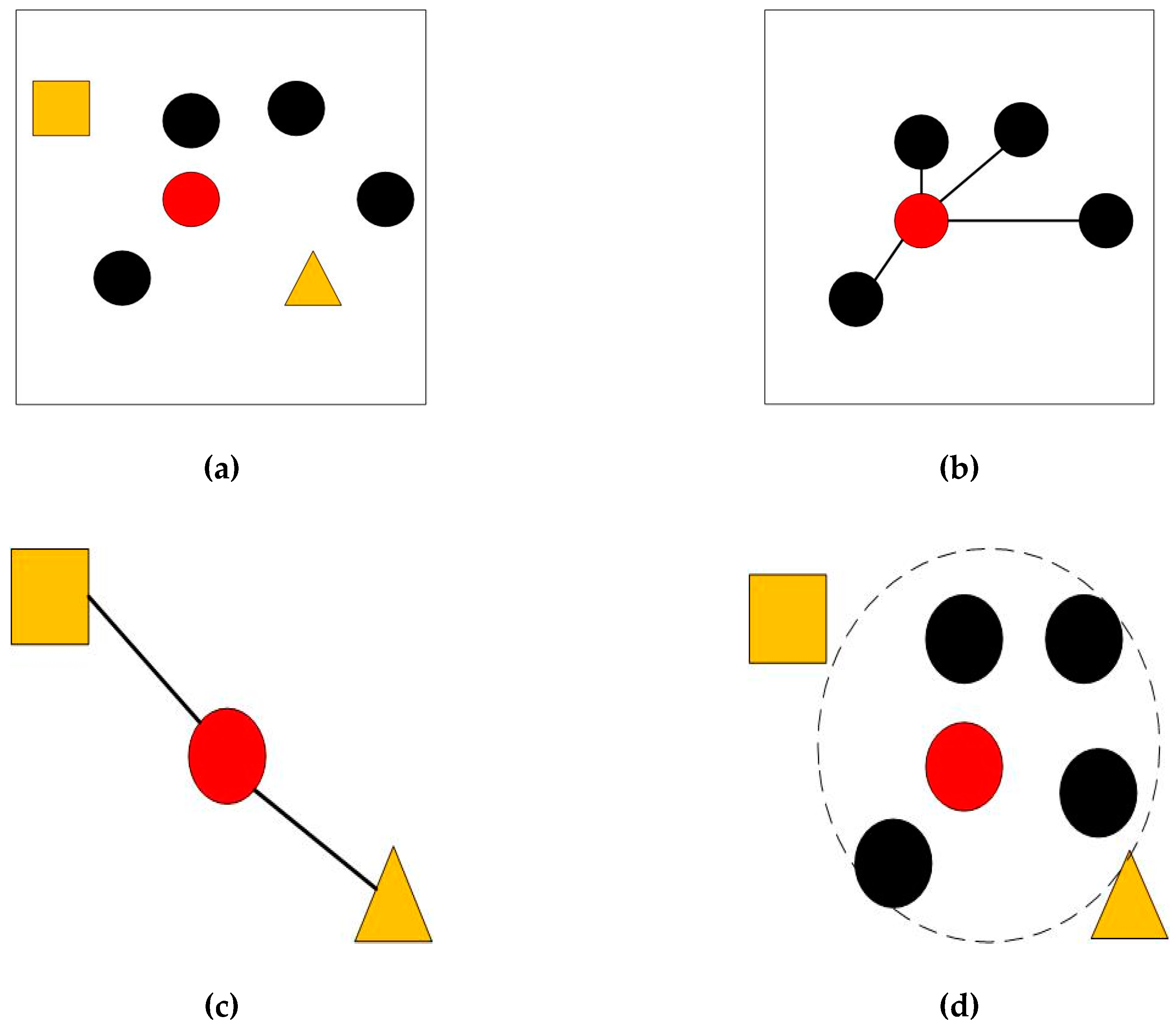
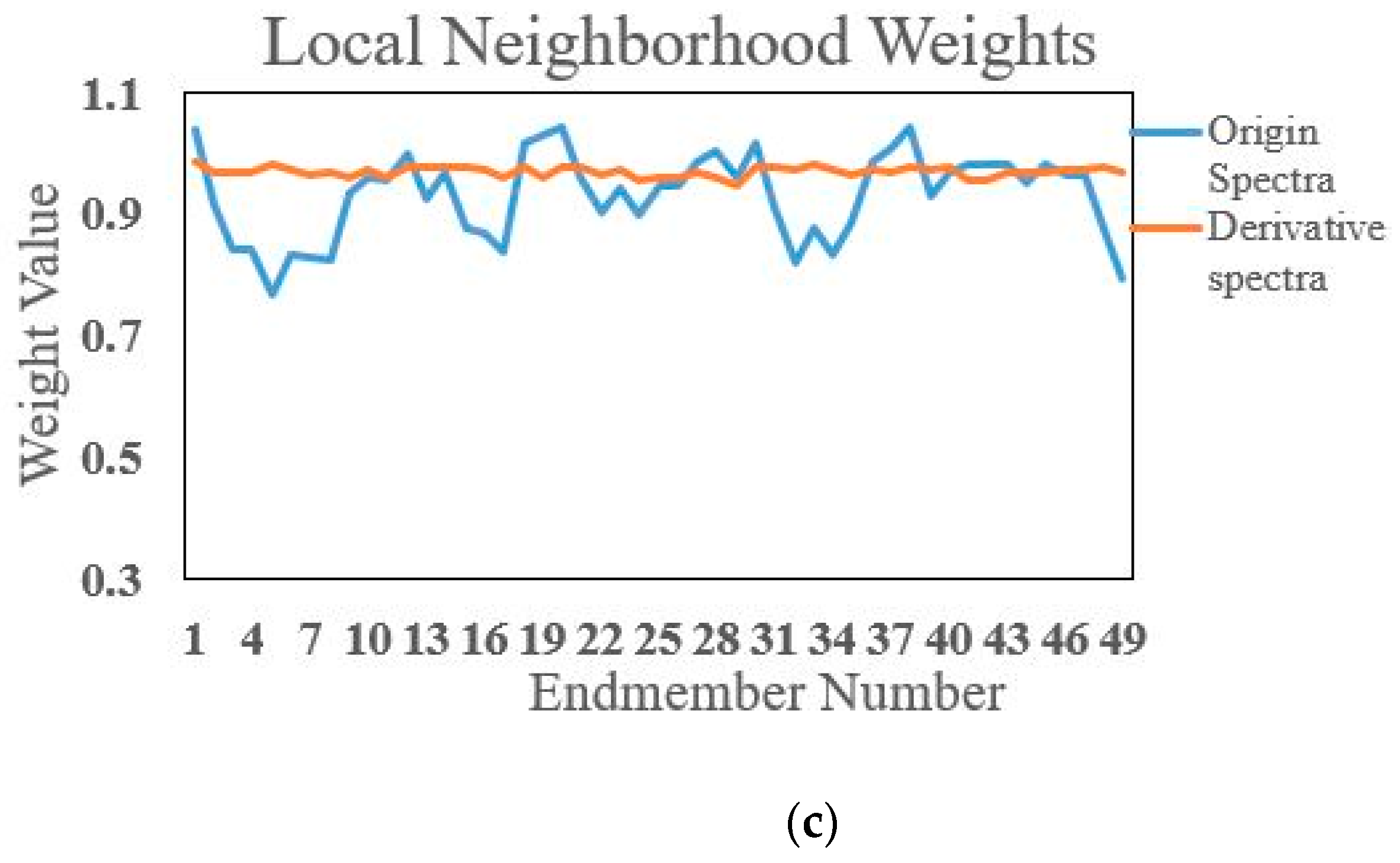
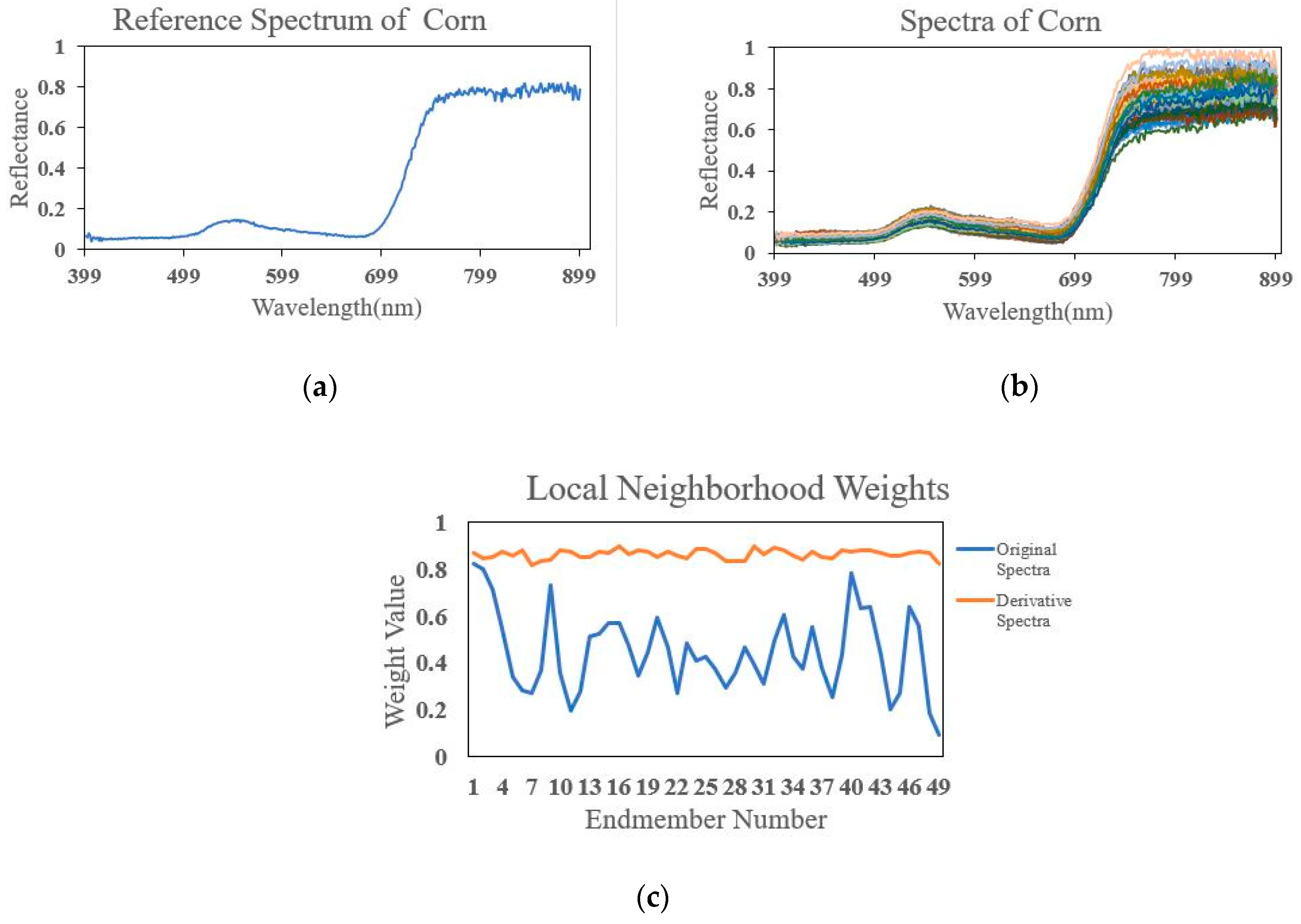
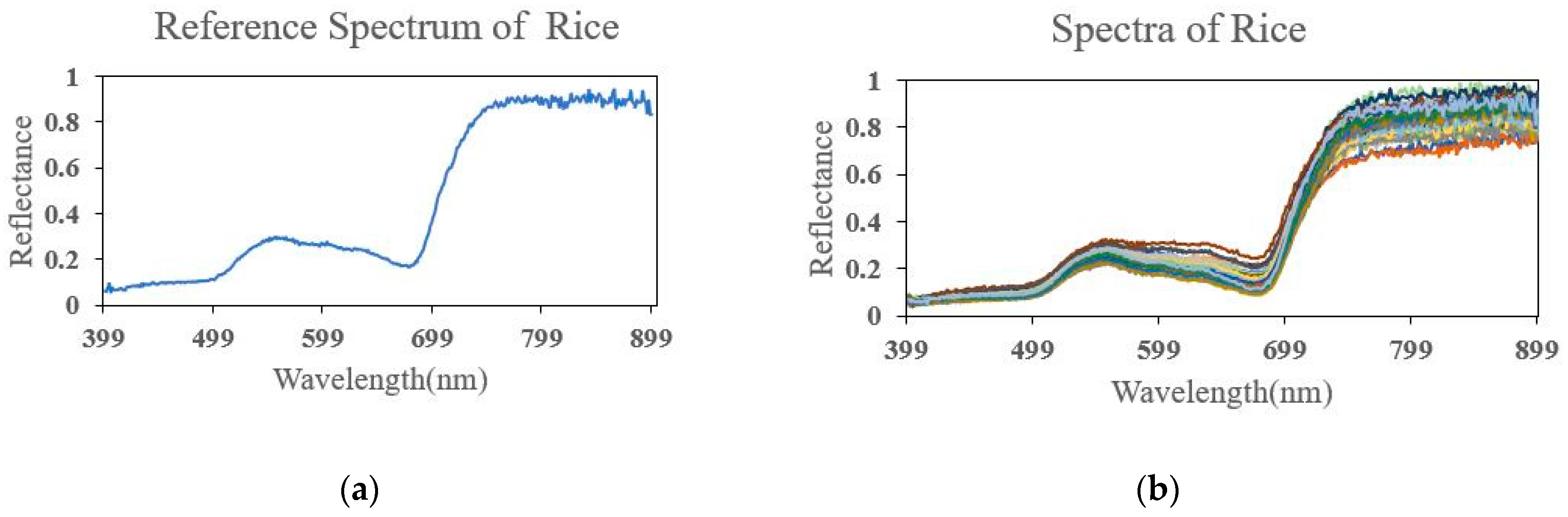
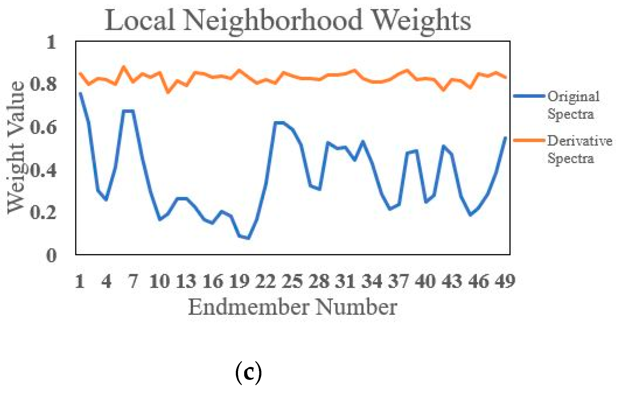
2.4. Local Neighborhood Derivative Weights

Derivative analysis of spectra has been used in hyperspectral remote sensing [22,36]. Derivative analysis can help deal with the overlapping spectral features and enhance spectral contrast, thereby improving the target identification accuracy. Derivatives of spectra are relatively insensitive to variations in illumination intensity caused by changes in sun angle, cloud cover, or topography [37]. Thus, first-order derivative spectra reduce the intra-class difference and increase the inter-class differences. First- and second-order derivative spectra have been applied to improve the estimation of sediment in water [38].

Spectra extracted from hyperspectral images consist of reflection values corresponding to different bands $\left(\lambda \right)$, which can be expressed in discrete forms:

$$\mathit{x}=\left[x\left({\lambda }_1\right),x\left({\lambda }_2\right),\dots ,x\left({\lambda }_L\right)\right]$$

(11)

where $\mathit{x}$ is the spectrum and $x\left({\lambda }_{\mathrm{i}}\right)$ is the reflectance value at wavelength ${\lambda }_{\mathrm{i}}$.

The first-order derivative spectrum can be calculated by the following Equation (12).

$${\mathit{x}}^{\prime }=\left[\frac{x\left({\lambda }_2\right)-x\left({\lambda }_1\right)}{{\lambda }_2-{\lambda }_1},\frac{x\left({\lambda }_3\right)-x\left({\lambda }_2\right)}{{\lambda }_3-{\lambda }_2},\dots ,\frac{x\left({\lambda }_L\right)-x\left({\lambda }_{L-1}\right)}{{\lambda }_L-{\lambda }_{L-1}}\right]$$

(12)

Since the enhancement of noise caused by differentiation is largely related to high-frequency noise [22], the Savitzky–Golay smoothing filter [39] is used to remove the high-frequency noise before calculating the first-order derivative spectrum.

Derivative analysis and local neighborhood weights are merged into local neighborhood derivative weights in the proposed method. First-order derivative spectrum is brought into modeling local neighborhood weights. The local neighborhood derivative weights act as regularization terms to penalize different abundance vectors. The first law of geography is expressed as “Everything is related to everything else, but near things are more related than distant things” [40]. Inspired by the first law of geography, the hyperspectral image is divided into multiple local windows. Figure 4 displays the diagram of the local window. It is assumed that the hyperspectral image with r×s pixels (r represents the length of the image; s represents the width of the image) is arranged on r×s circles. The spatial coordinate of the top left corner circle is (0,0), and the spatial coordinate of the bottom right corner grid is (r,s). In Figure 4, a black circle and red circles constitute a local window where the black circle represents central pixel and red circles represent neighboring pixels. Suppose that pixel ${\mathit{x}}_{\mathrm{i}}$, represented by the black circle, is set as the central pixel of the local window in Figure 4. If the pixel ${\mathit{x}}_{\mathrm{j}}$, represented by the red circle, is the neighboring pixel of pixel ${\mathit{x}}_{\mathrm{i}}$, we define $j\in N\left(i\right)$. If the pixel ${\mathit{x}}_j$, represented by the colorless circle, is not neighboring pixel of pixel ${\mathit{x}}_i$, we define $j\notin N\left(i\right).$

Local neighborhood derivative weights are expressed in Equation (13). The local neighborhood derivative weights can measure the similarity of the neighboring pixels to the center pixel. The form of local neighborhood derivative weights approximates the heat kernel [41], but the difference is that local neighborhood derivative weights use the derivative of the original spectrum to calculate the weight.

$$W_{ij}=K_{\sigma }\left({\mathit{x}}_i,{\mathit{x}}_j\right)=\{\begin{array}{c}{e}^{-\frac{\Vert {\mathit{x}}_{\mathit{i}}^{\prime }-{\mathit{x}}_{\mathit{j}}^{\prime }\Vert {}^2}{\sigma }},j\in N\left(i\right)\\ \\ 0, j\notin N\left(i\right)\end{array}$$

(13)

where σ is a scaling parameter of the local neighborhood derivative weight. ${\mathit{x}}_i$,${\mathit{x}}_j$ are the i^th and j^th original spectrum vectors of the hyperspectral image $\mathit{X}$. ${\mathit{x}}_{\mathit{i}}^{\prime },{\mathit{x}}_{\mathit{j}}^{\prime }$ are the first-order derivative spectrum of ${\mathit{x}}_i$,${\mathit{x}}_j$. When the pixel ${\mathit{x}}_j$ locates inside the local window, its degree of similarity to the center pixel ${\mathit{x}}_i$ can be calculated using local neighborhood derivative weights. When the pixel ${\mathit{x}}_j$ locates outside of the local window, its degree of similarity to the center pixel does not need to be calculated. This is in line with the expression of the first law of geography. The σ value is expressed as follows:

$$\sigma =\frac{1}{h-1}{\displaystyle \sum }_{j\in N\left(i\right)}\Vert {\mathit{x}}_{\mathit{i}}^{\prime }-{\mathit{x}}_{\mathit{j}}^{\prime }\Vert {}^2$$

(14)

where h denotes the number of neighboring pixels in the local window.

Noted that the spectra of rock extracted from hyperspectral image vary in Figure 5. One of the rock spectra is selected as reference spectrum. Reference original spectrum and other original spectra are used to compute local neighborhood weights according to Equation (13). The same arithmetic operation works on reference derivative spectrum and other derivative spectra. The results are shown in Figure 5c. The conclusion that local neighborhood derivative weights are insensitive to ESV can be obtained by comparing with results of original spectra and derivative spectra.

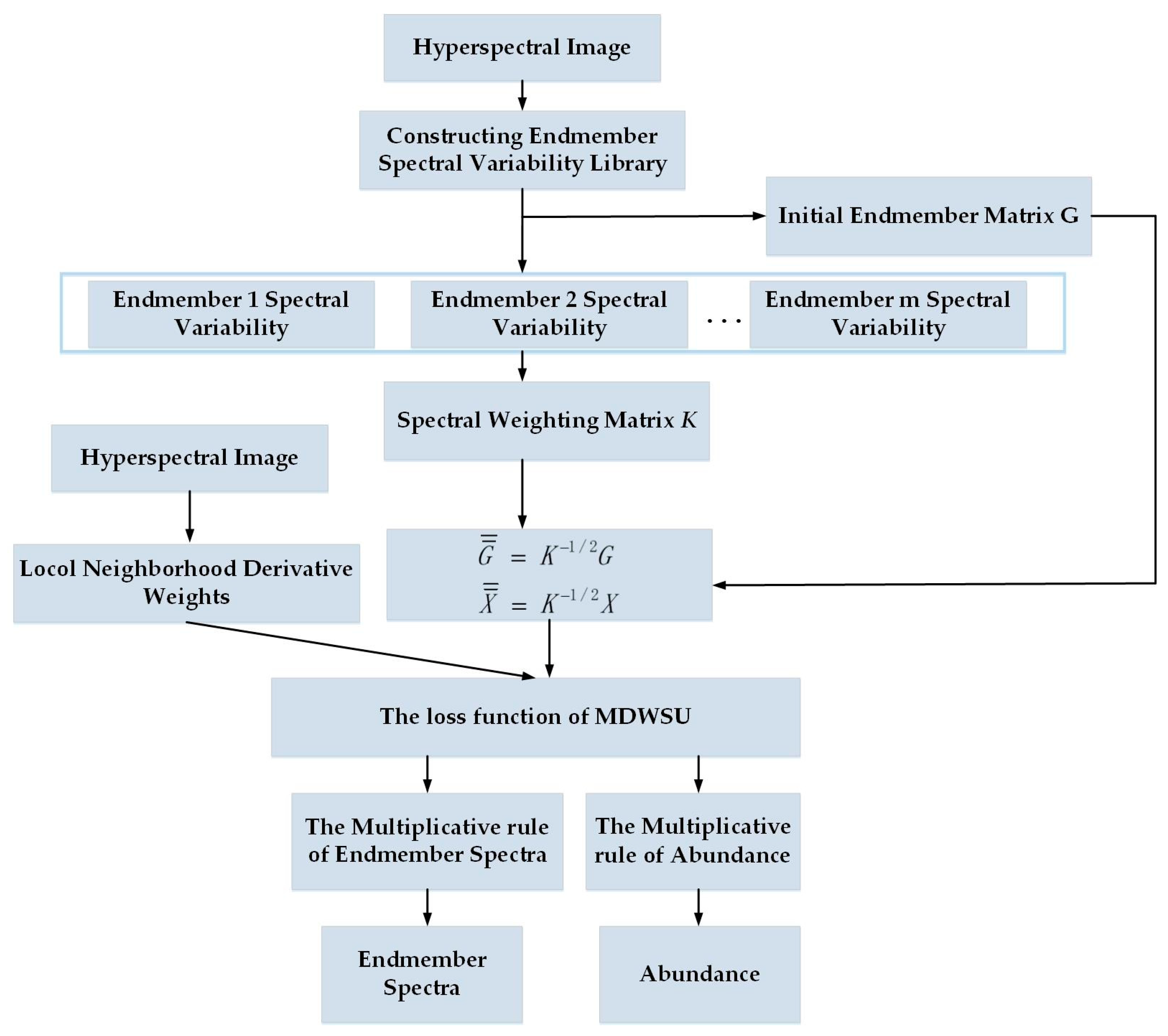
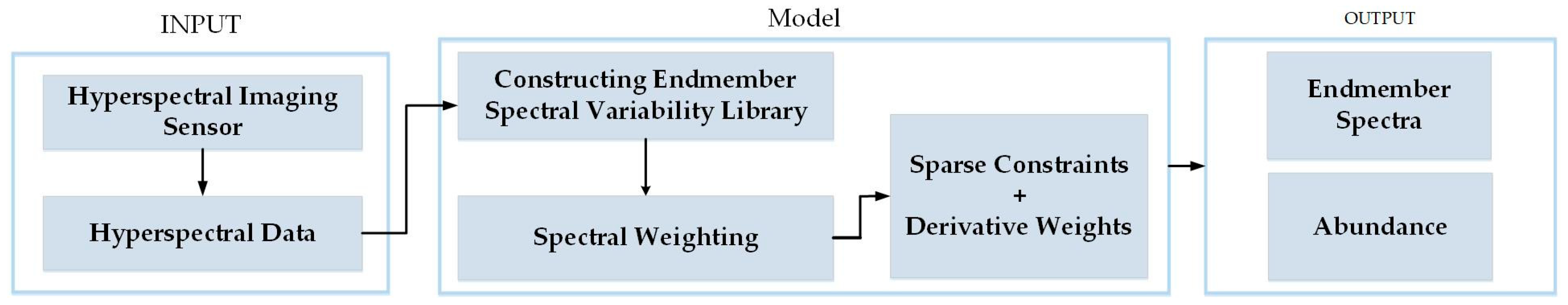
2.5. The Proposed MDWSU Algorithm Model

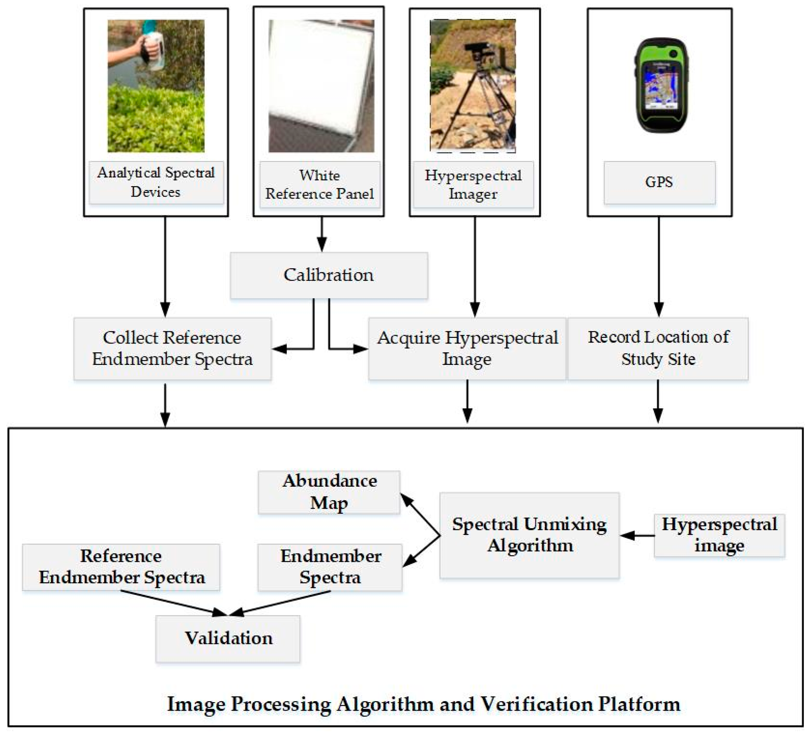
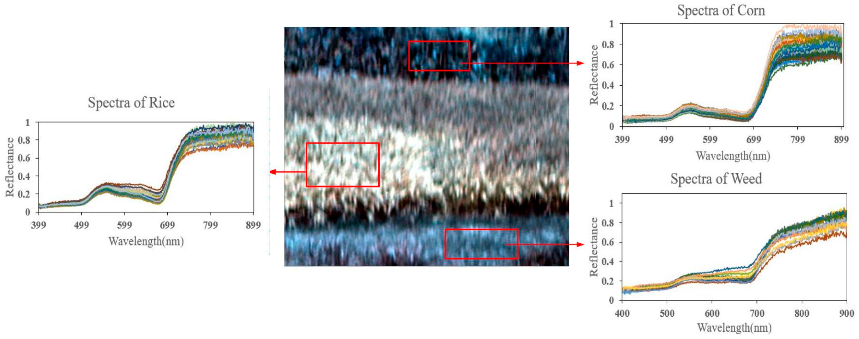
Spectral unmixing aims to obtain endmember spectra and corresponding abundance fraction from hyperspectral image. Non-negative matrix factorization (NMF) has been widely under research in the field of spectral unmixing. During the spectral unmixing process, NMF finds the appropriate endmember matrix $\stackrel{=}{\mathit{G}}$ and abundance A to minimize the difference between $\stackrel{=}{\mathit{X}}$ and $\stackrel{=}{\mathit{G}}\mathit{A}$. The difference between $\stackrel{=}{\mathit{X}}$ and $\stackrel{=}{\mathit{G}}\mathit{A}$ can be measured in terms of Euclidean distance. The loss function of NMF based on Euclidean distance is as follows:

$$\underset{\mathit{G},\mathit{A}}{\min }f\left(\mathit{G},\mathit{A}\right)=\Vert \stackrel{=}{\mathit{X}}-\stackrel{=}{\mathit{G}}\mathit{A}\Vert {}_F^2$$

(15)

where the operator ‖.‖_F represents the Frobenius norm.

Due to the non-convexity of NMF, it is difficult to obtain the global optimal solution [42]. Since the solution obtained by NMF is not unique, other constraints are often introduced into NMF, such as non-negative matrix factorization with minimum volume constraints (MVC-NMF) [43]. To improve the sparsity of abundance, the proposed method introduces abundance sparsity constraints into NMF. The L_1/2 regularizer has been proven to provide the best sparse solution [42]. Using the L_1/2 regularizer as sparsity constraints, NMF with sparsity constraints is written as:

$$\underset{\mathit{G},\mathit{A}}{\min }f\left(\mathit{G},\mathit{A}\right)=\Vert \stackrel{=}{\mathit{X}}-\stackrel{=}{\mathit{G}}\mathit{A}\Vert {}_F^2+\lambda {\Vert \mathit{A}\Vert }_{1/2}$$

(16)

where $\lambda$ is the regularization parameter. ${\Vert \mathit{A}\Vert }_{1/2}$ is defined in the Equation (17).

$${\Vert \mathit{A}\Vert }_{1/2}={\displaystyle \sum }_{i=1}^m{\displaystyle \sum }_{j=1}^n{\Vert \mathit{A}\Vert }_{ij}^{1/2}$$

(17)

The parameter λ depends on the sparsity of abundances. Since these abundances cannot be obtained a priori, we use a rough estimator for λ defined in Equation (18) based on the sparseness criteria in [42].

$$\lambda =\frac{1}{\sqrt{l}}{\displaystyle \sum }_{i=1}^l\frac{\sqrt{n}-\Vert {\mathit{X}}_i\Vert {}_1/\Vert {\mathit{X}}_i\Vert {}_2}{\sqrt{n-1}}$$

(18)

where ${\mathit{X}}_i$ denotes the i^th band data of hyperspectral image, the operator ‖.‖₁ represents the matrix 1-norm and the operator ‖.‖₂ represents the matrix 2-norm.

There exists a close link between hyperspectral image and decomposed abundance matrix [44]. The more similar the neighboring pixel to the central pixel is, the more similar the abundance of the neighboring pixel is to the abundance of the central pixel. Once the derivative of neighboring pixel is similar to the derivative of central pixel, the abundance of neighboring pixel is close to the abundance of central pixel. Considering the similarity between the abundance of neighboring pixels and the central pixel, the local neighborhood derivative weight regularization for guaranteeing abundance smoothness is written as:

$$\begin{gathered} {\displaystyle \sum }_{i=1}^n{\displaystyle \sum }_{j\in N\left(i\right)}\Vert {\mathit{a}}_i-{\mathit{a}}_j\Vert {}^2{W}_{i,j}={\displaystyle \sum }_{i=1}^n{\mathit{a}}_i^T{\mathit{a}}_i{\mathit{D}}_{ii}-{\displaystyle \sum }_{i=1}^n{\displaystyle \sum }_{j\in N\left(i\right)}{\mathit{a}}_i^T{\mathit{a}}_j{\mathit{W}}_{i,j} \\ =\mathrm{Tr}\left(\mathit{A}\left(\mathit{D}-\mathit{W}\right){\mathit{A}}^T\right) \end{gathered}$$

(19)

where $\mathrm{Tr}(.)$ represents the trace of matrix, $\mathit{W}$ is weight matrix in which ${\mathit{W}}_{i,j}$ is element, D is a diagonal matrix, and ${\mathit{D}}_{ii}={{\displaystyle \sum }}_{j\in N\left(i\right)}{\mathit{W}}_{i,j}$.

Then the local neighborhood derivative weight regularization is incorporated into the Equation (16). The loss function of MDWSU based on Euclidean distance is written as:

$$\underset{\mathit{G},\mathit{A}}{\min }f\left(\mathit{G},\mathit{A}\right)=\Vert \stackrel{=}{\mathit{X}}-\stackrel{=}{\mathit{G}}\mathit{A}\Vert {}_F^2+\lambda {\mathit{A}}_{1/2}+\frac{\mu }{2}\mathrm{Tr}\left(\mathit{A}\left(\mathit{D}-\mathit{W}\right){\mathit{A}}^T\right)$$

(20)

where $\mu \ge 0$ is the regularization parameter of the local neighborhood derivative weight regularization.

Subsequently, the multiplicative update rules [45] is adopted to solve the MDWSU model. The multiplicative update rules are as follows:

$$\stackrel{=}{\mathit{G}}\leftarrow \stackrel{=}{\mathit{G}}.\ast (\stackrel{=}{\mathit{X}}{\mathit{A}}^T)./(\stackrel{=}{\mathit{G}}\mathit{A}{\mathit{A}}^T)$$

(21)

$$\mathit{A}\leftarrow \mathit{A}.\ast ({\stackrel{=}{\mathit{G}}}^T\stackrel{=}{\mathit{X}}+\mu \ast \mathit{A}\ast \mathit{W})./({\stackrel{=}{\mathit{G}}}^T\stackrel{=}{\mathit{G}}\mathit{A}+0.5\ast \lambda {\mathit{A}}^{-\frac{1}{2}} +\mu \ast \mathit{A}\ast \mathit{D})$$

(22)

where $.\ast$ and $./$ represent element-wise division operation and element-wise division operation, respectively. The details of the multiplicative update rules and the implementation issue of the MDWSU model are presented in the Appendix A.

The flowchart of the proposed method is shown in Figure 6.

3. Data Acquisition

We choose the right place as the study site and obtain the hyperspectral images preparing for verifying the effectiveness of the proposed method.

Hyperspectral data acquisition system and data processing flow is illustrated in Figure 7. Hyperspectral data acquisition system consists of Analytical Spectral Devices (ASD), white reference panel, hyperspectral imager and GPS. GPS is used to record the geographical location of study site. FieldSpec Handheld2 Spectroradiometer is selected as ASD. The ground object spectra are measured using ASD. The ASD can measure the reflected electromagnetic radiance of ground objects covering the wavelength ranging from 325 nm to 1075 nm with spectral resolution superior to 3 nm in the field. The white reference panel is used to calibrate the ground object spectrum measurement every ten minutes to guarantee measurement accuracy. In addition, the spectrum of each ground object was measured ten times. During the acquisition of the sample spectrum, the distance between the acquisition target area and the ASD is between 0.5 and 1.0 m, and the acquisition target area should be within the 25° field of view in the lowest point of the ASD. A Resonon Pika XC2 hyperspectral imager is chosen to acquire hyperspectral images. The hyperspectral imager is a push-broom imager and used to acquire visible and near-infrared hyperspectral imagery with the wavelength ranging from 400 nm to 1000 nm. The hyperspectral imager has 462 spectral channels with 1.3 nm spectral resolution and 1600 spatial channels. The hyperspectral imager weights 2.2 kg and its dimensions are 10.1 cm × 27.5 cm × 7.4 cm.

We chose two places in Jiangxi Province as research sites, whose latitude and longitude are (29.35°N, 118.09°E) and (29.04°N, 117.74°E), respectively. The first study site covered by corn, rice and weed is shown in Figure 8. The hyperspectral dataset in Figure 8 consists of 400 × 400 pixels. The second study site containing vegetation, tidal flats and water is shown in Figure 9. The hyperspectral dataset in Figure 9 consists of 158 × 178 pixels. We used hyperspectral imager to acquire visible and near-infrared hyperspectral imagery with the wavelength ranging from 400 nm to 1000 nm in the above-mentioned two places in September 2017. Then we used a white reference panel to calibrate original hyperspectral images and converted the hyperspectral images from radiance to reflectance. There are 462 channels in hyperspectral images. Channels 1–12 and 385–462 were abandoned due to the hyperspectral imaging sensor noise and water vapor absorption in the atmosphere. As a result, channels 13–384 of hyperspectral images ranging from 400 nm to 900 nm were used to verify the algorithm.

4. Experimental Results and Analysis

To verify the effectiveness of the MDWSU algorithm model, the accuracy of unmixing results is evaluated using the spectral angle distance (SAD), and the root mean square error (RMSE). We use spectral angle distance (SAD) to measure the extent to which the estimated endmember spectrum approximates to the true endmember spectrum. SAD is expressed in the following Equation (23).

$$SA{D}_i=arccos\left(\frac{{\mathit{g}}_i{}^T\widehat{{\mathit{g}}_i}}{\Vert {\mathit{g}}_i{}^T\Vert \hspace{1em}\Vert \widehat{{\mathit{g}}_i}\Vert }\right)$$

(23)

where ${\mathit{g}}_i$ is the i^th estimated endmember signature and $\widehat{{\mathit{g}}_i}$ is the i^th true endmember signature. The smaller the SAD value is, the more the estimated endmember is similar to the true spectrum.

The root mean square error (RMSE) of the entire hyperspectral image is written as:

$$\mathrm{RMSE}=\frac{1}{n}{{\displaystyle \sum }}_{i=1}^n\sqrt{\frac{1}{l}{{\displaystyle \sum }}_{j=1}^l{\left({\mathit{X}}_{i,j}-{\left(\mathit{G}\cdot \mathit{A}\right)}_{i,j}\right)}^2}$$

(24)

where n denotes the number of the total pixels of hyperspectral image and $l$ denotes the number of the total bands of hyperspectral image. RMSE measures the error between the original hyperspectral image and reconstructed image. If the calculated RMSE is smaller, the accuracy of the decomposed abundance matrix and endmember matrix is higher. In general, since the model errors intend to obey normal distribution, RMSE is a good metric of model performance [46].

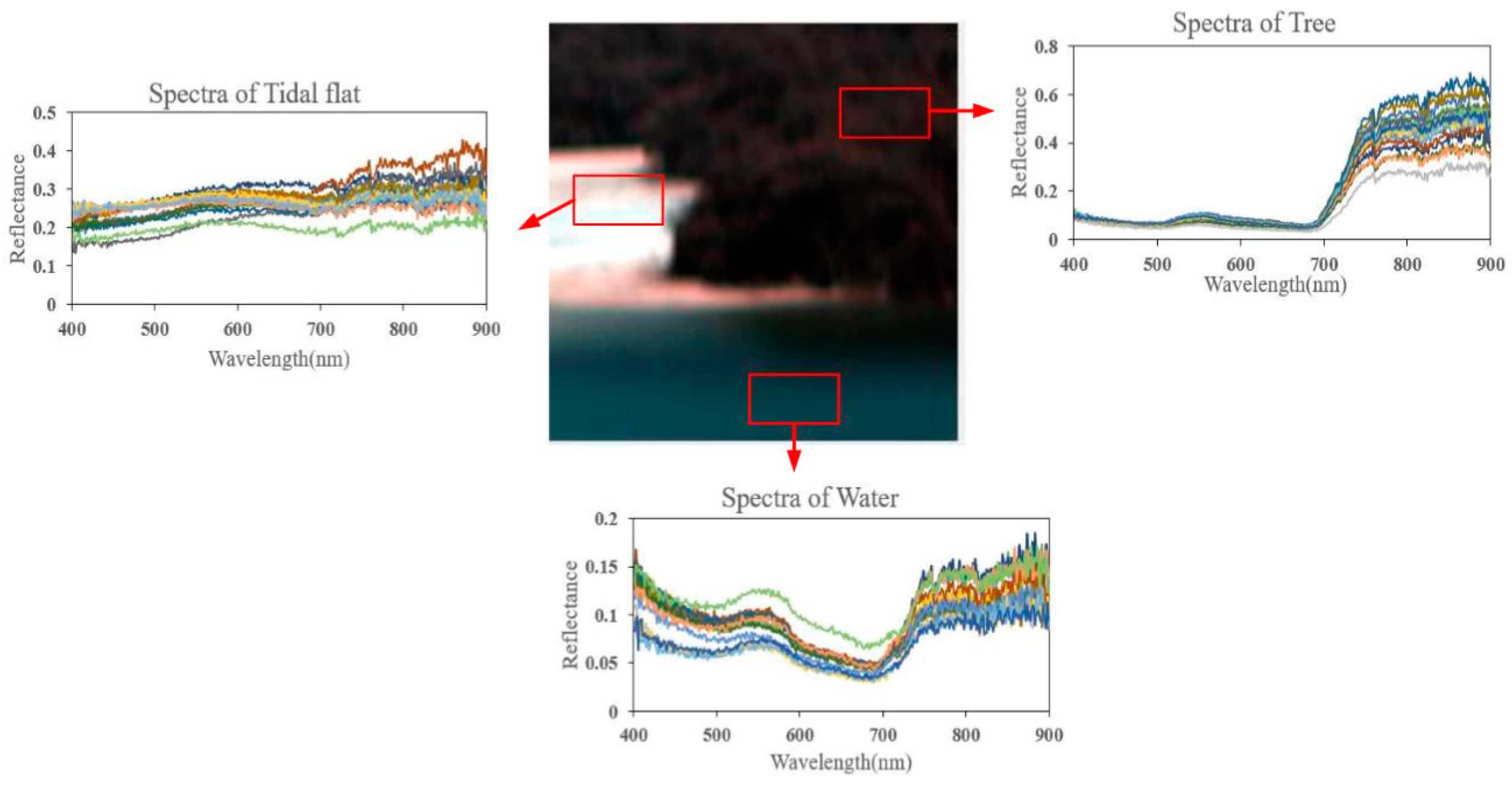
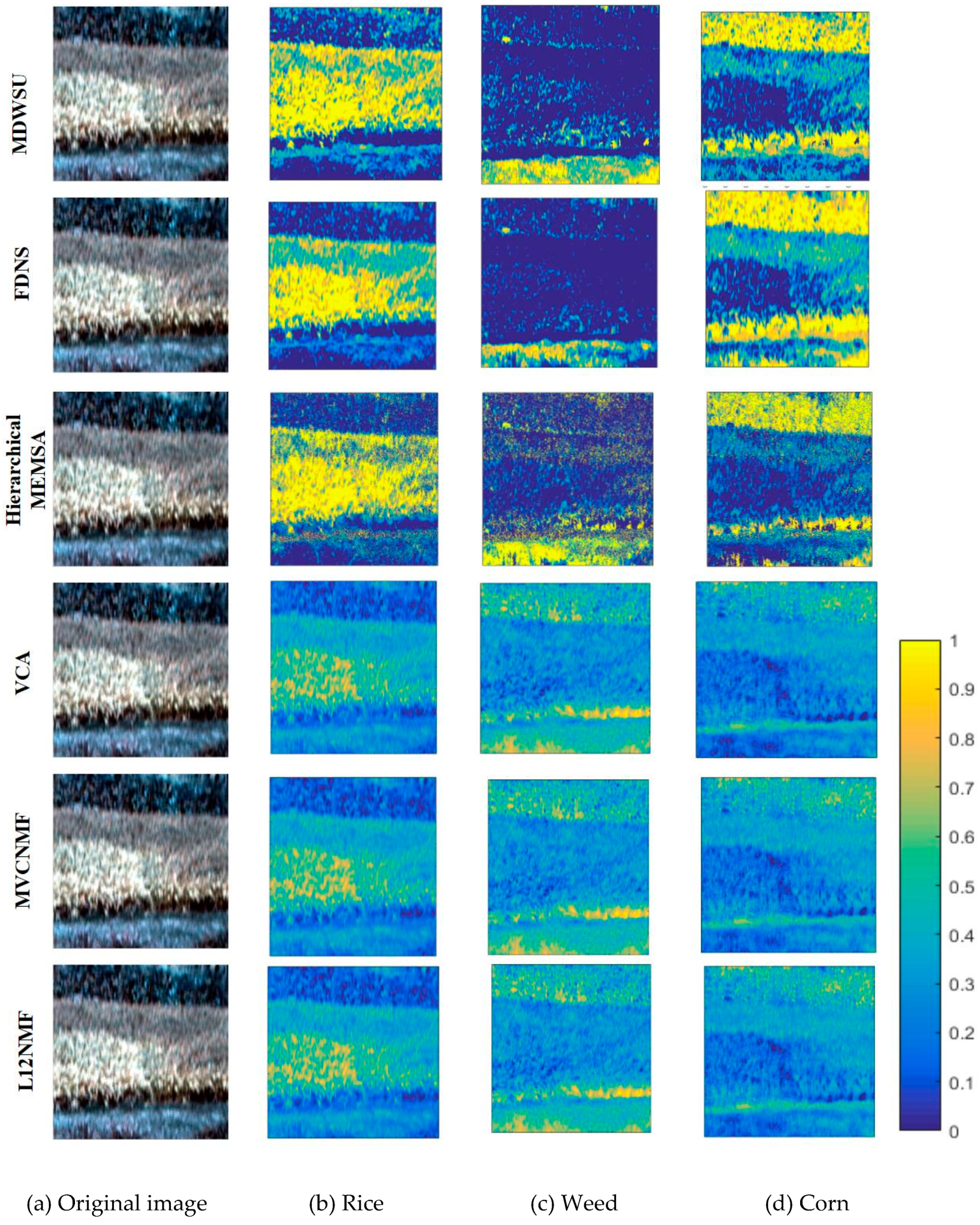
4.1. Real Hyperspectral Data Experiments

Two different real hyperspectral datasets acquired by Resonon Pika XC2 hyperspectral imager are used to verify the effectiveness of the MDWSU method. Sixty spectra for each endmember are obtained by ASD. Then average values of spectra obtained by ASD for each endmember are adopted as the reference endmember spectra. Figure 8 shows the real hyperspectral image of the first study site (29.35°N, 118.09°E) near Wuyuan district of Jiangxi Province in China, which is covered by the rice, corn, and weed. Figure 9 shows another real hyperspectral image of the second study site (29.04°N, 117.74°E) near Dexing district of Jiangxi Province in China, which is covered by tidal flats, vegetation, and water. In this section, these two hyperspectral images are experimented with different algorithms.

The MDWSU model method is compared with Fisher discriminant null space (FDNS) [25], hierarchical MEMSA [12], VCA with fully constrained least squares (FCLS) [47], non-negative matrix factorization with minimum volume constraints (MVC-NMF) [43], and non-negative matrix factorization with sparsity constraints (L_1/2-NMF) [42]. FDNS and hierarchical MEMSA have been developed to deal with endmember spectral variability, while the other three methods are traditional methods which assume that each endmember must have only one constant spectral signature. The FDNS searches a linear transformation of the spectra, from the original sample space to a lower dimensional space, which reduces the intra-class spectral differences in the low dimensional space [25]. The hierarchical MEMSA here is adopted to compare the abundance fractions accuracy with the MDWSU model. A spectral library containing different endmembers adapted to different scenes was created from the image by human visualization. Three endmember selection procedures (Endmember Average Root Mean Square Error, Minimum Average Spectral Angle, and Count Based Endmember Selection) were used to identify the most representative endmembers from the spectral library for each class [12]. The VCA algorithm is widely used to compare spectral unmixing performance due to its relatively high precision and stability. NMF has drawn much attention in the field of hyperspectral remote sensing [48]. When it is applied to spectral unmixing, auxiliary constraints are introduced into NMF algorithm, making the model in line with real geographical significance. Taking the attributes of endmember signatures and abundance fractions into account, algorithms with different constraints have been developed for spectral unmixing. The constraints for NMF-based spectral unmixing algorithms are mainly classified into two categories: spectral-based constraints and abundance-based constraints. MVC-NMF is a classic algorithm of NMF with the spectral-based constraints while L_1/2-NMF is a typical algorithm of NMF with the abundance-based constraints.

Figure 10 displays the abundance fractions of the MDWSU model and the other methods. Evaluating abundance maps by visual interpretation method, the best abundance estimation is achieved by the MDWSU model, yet there are some obvious errors in the abundance maps of other methods. As the spectra of the weeds and crops are highly similar, traditional unmixing methods (i.e., VCA-FCLS, MVC-NMF, and L_1/2-NMF) cannot distinguish them effectively, so an incorrect abundance estimation of weed and corn corresponding to VCA-FCLS, MVC-NMF, and L_1/2-NMF algorithms exists in Figure 10. Some weeds with high abundance exist in the corn abundance map obtained by the FDNS algorithm, which is obviously not in line with actual situation. As the spectral transformation of the FDNS algorithm is a dimensionality reduction algorithm, the linearly transformed low-dimensional spectral information loses the information of the original spectrum that can effectively distinguish between corn and weeds. There are many errors in the weed and corn abundance maps of the Hierarchical MEMSA algorithm. However, the MDWSU algorithm constructs spectral weighting matrix assigning different weights to different bands, which enlarges the inter-class differences and decreases intra-class differences. Furthermore, the local neighborhood derivative weights allow the abundance of similar ground objects close. The MDWSU algorithm model can obtain better abundance estimation results than other methods.

Figure 11 displays the abundance maps of the proposed method and other algorithms. The MDWSU model estimates better than other algorithms referring to tree and water abundance fraction maps. In the water abundance fraction maps, the other algorithms misidentified the tree as water, yet the MDWSU model avoided this error. As the tree shadow spectrum is close to the water spectrum in spectral magnitude, so the error appears in the water abundance of other algorithms. Although the spectral curve of water is close to the spectral curve of the tree shadow, the spectral curves of the tree shadow and the trees are substantially coincident in the bands between 400 nm and 700 nm. Other algorithms cannot effectively use the above-mentioned information to distinguish between trees, tree shadow, and water, so the tree shadows are classified as water. Tree shadows are classified as trees rather than water in the MDWSU model.

Table 1. Spectral angle distance (SAD) results of first real hyperspectral data (the best results are denoted by bold font).

	MDWSU	FDNS	L1/2-NMF	MVC-NMF	VCA-FCLS
Rice	0.1654	0.2354	0.4597	0.2380	0.2056
Corn	0.1921	0.1975	0.5632	0.2076	0.3421
Weed	0.2072	0.2236	0.3216	0.3154	0.1768
AVERAGE	0.1882	0.2188	0.4481	0.2536	0.2418

,

Table 2. Root mean square error (RMSE) results of first real hyperspectral data (the best results are denoted by bold font).

MDWSU	FDNS	Hierarchical MEMSA	L1/2-NMF	MVC-NMF	VCA-FCLS
0.0075	0.0088	0.0087	0.0106	0.0097	0.0118

,

Table 3. SAD results of second real hyperspectral data (the best results are denoted by bold font).

	MDWSU	FDNS	L1/2-NMF	MVC-NMF	VCA-FCLS
Water	0.1135	0.2142	0.3278	0.3876	0.5310
Tree	0.1218	0.1882.	0.4571	0.4782	0.4674
Tidal flat	0.0712	0.2537	0.1037	0.0958	0.0897
AVERAGE	0.1021	0.2187	0.2962	0.3205	0.3627

, and

Table 4. RMSE results of second real hyperspectral data (the best results are denoted by bold font).

MDWSU	FDNS	Hierarchical MEMSA	L1/2-NMF	MVC-NMF	VCA-FCLS
0.0063	0.0078	0.0075	0.0115	0.0124	0.0098

provide the SAD and RMSE values of different algorithms. The best results are denoted by bold font. The lower the SAD and RMSE values are, the more accurate the abundance estimation and endmember spectra estimation are. The average SAD and RMSE values of the MDWSU algorithm are the lowest compared with other algorithms, which proves the effectiveness of the proposed method. Endmember spectral variability widely exists in real hyperspectral images, especially in vegetation areas, which can be interpreted by illumination variation. Experimental results show that it is feasible to combine the spectral weighting matrix with local neighborhood derivative weights in reducing the effect of ESV on unmixing accuracy.

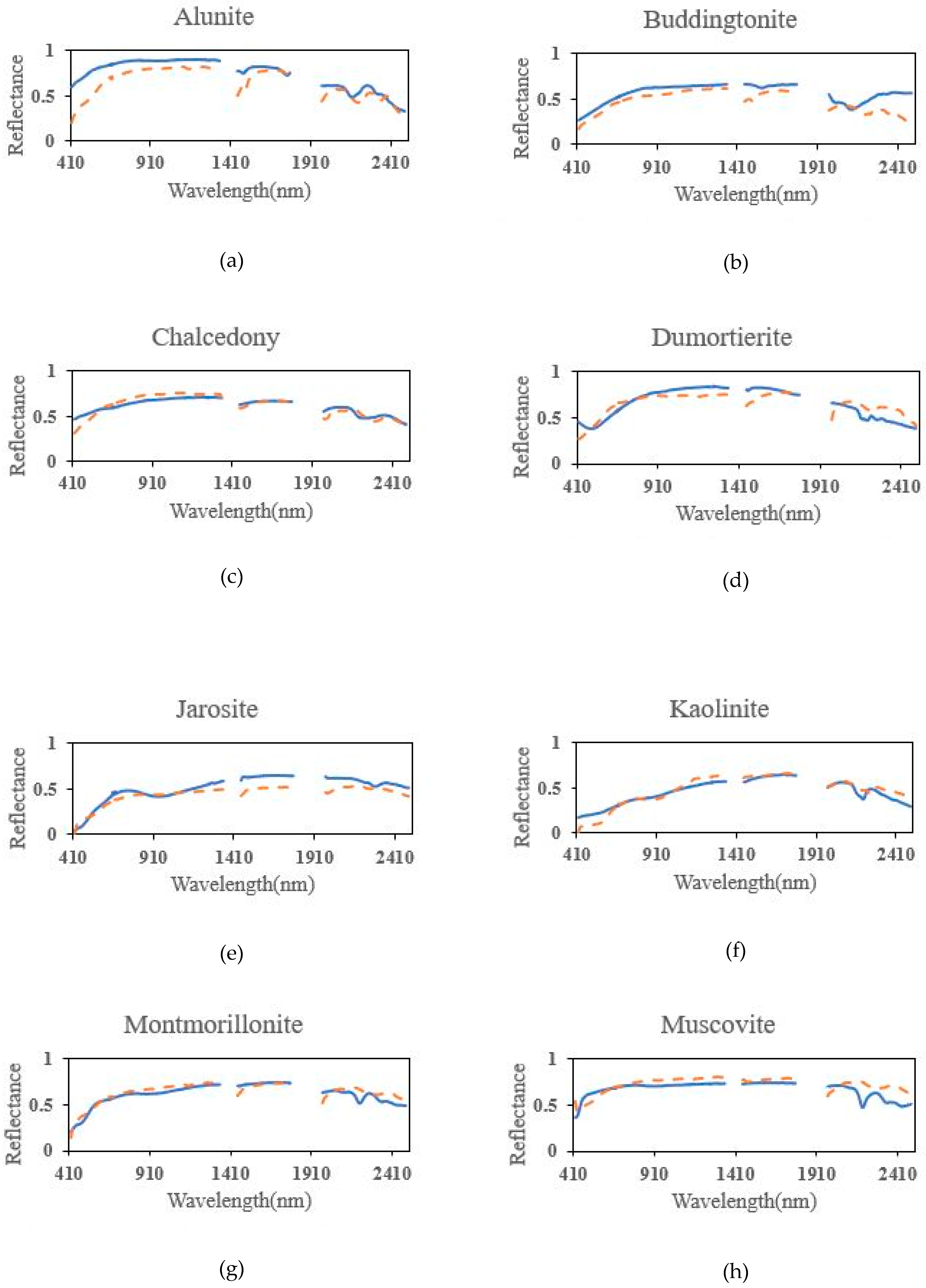
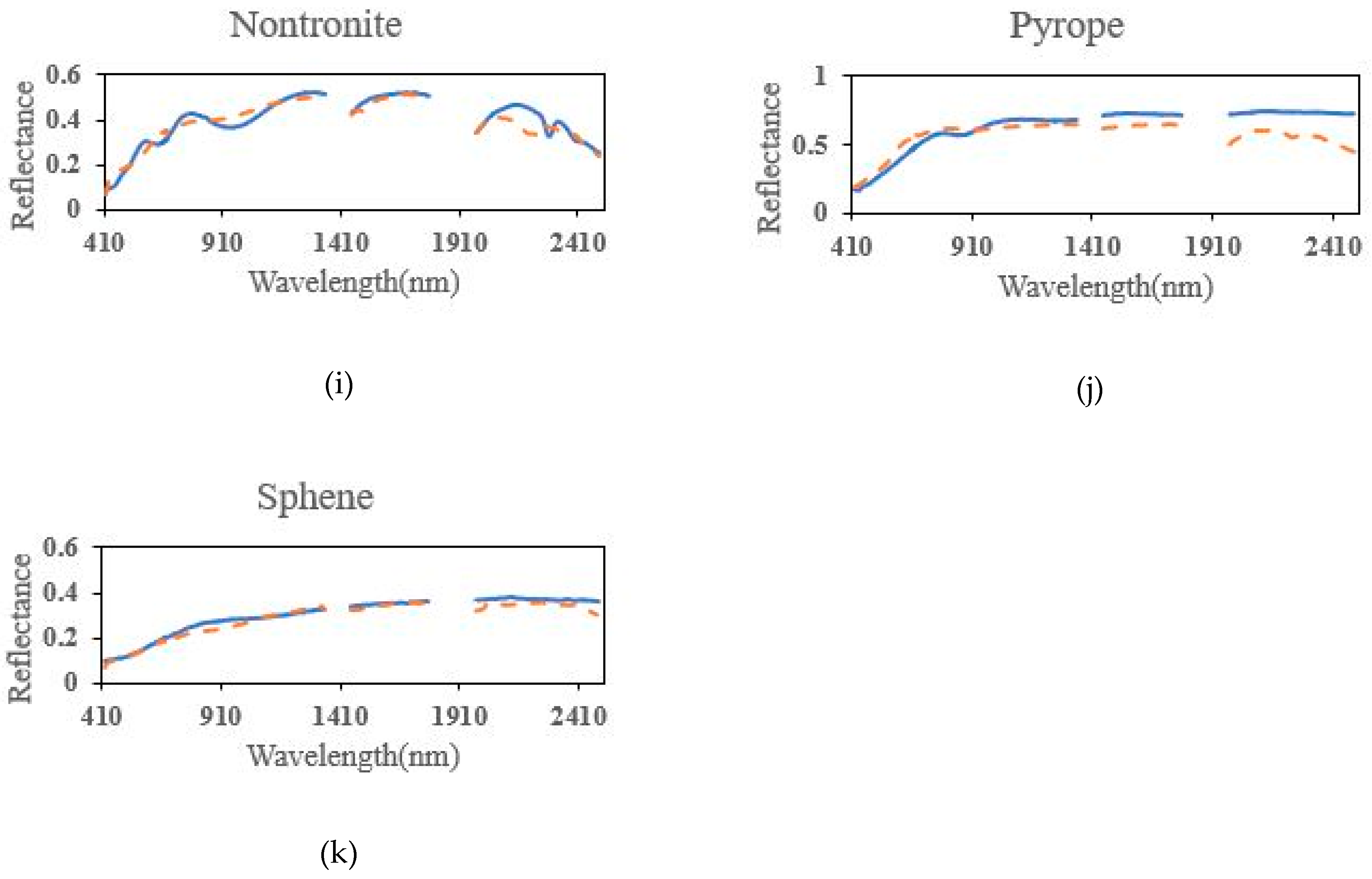
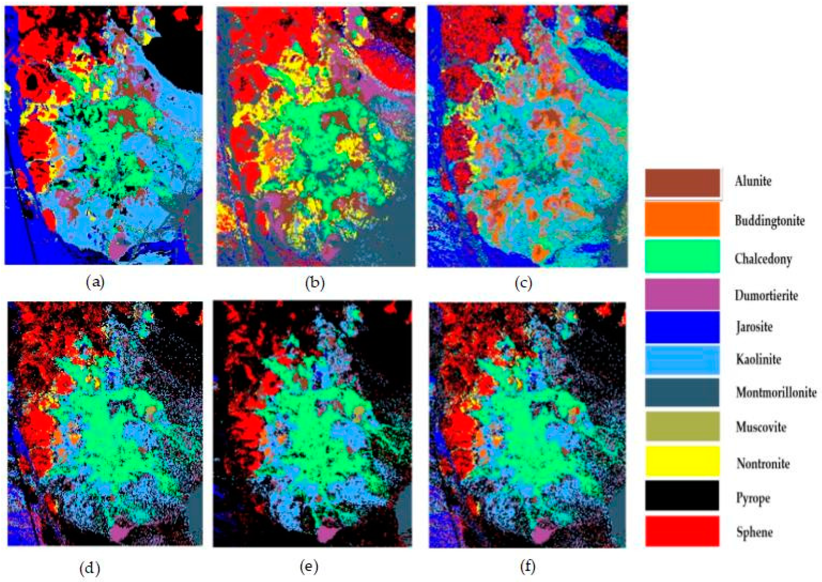
4.2. Experimental Results of the AVIRIS Cuprite Dataset

Another real hyperspectral data about the Cuprite mineral district will be used to verify the effectiveness of the MDWSU model. The Cuprite mineral district is located in the western part of Nevada, USA, which has been established as a mineralogical reference site for remote sensing instruments [49,50,51]. The image was acquired by an Airborne Visible-Near/Infrared Imaging Spectrometer (AVIRIS) sensor on 19 June 1997. The reference spectral library of minerals in Cuprite mineral district is available on the internet [52]. The MDWSU algorithm and other algorithms will extract endmembers from the Cuprite image. SAD is used to measure the accuracy of the estimated endmember spectra. The subimage with 250 × 190 pixels is intercepted from the raw hyperspectral data. Figure 12 displays false-color subimage of AVIRIS Cuprite data. In the AVIRIS Cuprite data, there are 224 spectral bands with the wavelength ranging from 400 nm to 2500 nm. In experiments, the low SNR bands and the water vapor absorption bands (1–2, 104–113, 148–167, and 221–224) have been removed [42]. Estimating the number of endmembers in the selected region is a challenging issue due to endmember spectral variability of the same mineral with different chemical compositions. Regarding the number of endmembers, different algorithms provide different estimations in the literature. To address the endmember spectral variability, human interpretation is needed for the estimation of the number of endmembers [53]. Referring to the existing analysis in [44], there are 11 different types of minerals in the scene. Furthermore, the estimated number of endmembers in the selected region is set to 11 via virtual dimensionality (VD) method [54] with false alarm probability $P_f={10}^{-8}$.

Figure 13 displays a comparison between the endmember spectra of the MDWSU algorithm and the USGS library. The endmember spectra of the MDWSU algorithm are displayed in orange dotted lines while the reference endmember spectra are shown in blue solid lines in Figure 13. Figure 14 shows the hard classification maps where the class label is assigned to a pixel in which the class having the highest abundance fraction. The hard classification maps in Figure 14 are obtained by MDWSU, FDNS, Hierarchical MEMSA, L_1/2-NMF, MVC-NMF, and VCA-FCLS.

Table 5. SAD results of the AVIRIS Cuprite data (the best results are denoted by bold font).

	MDWSU	FDNS	L1/2-NMF	MVC-NMF	VCA-FCLS
Alunite	0.1356	0.1245	0.1895	0.1965	0.1278
Buddingtonite	0.0967	0.0983	0.1269	0.1157	0.2638
Chalcedony	0.0981	0.0991	0.1104	0.1087	0.0931
Dumortierite	0.0827	0.1153	0.1371	0.0721	0.1288
Jarosite	0.0928	0.0986	0.1183	0.1212	0.1372
Kaolinite	0.0698	0.1181	0.1081	0.1279	0.1219
Montmorillonite	0.0564	0.0861	0.0937	0.0723	0.1752
Muscovite	0.0803	0.1035	0.0921	0.1327	0.1935
Nontronite	0.0741	0.0723	0.0901	0.0927	0.2649
Pyrope	0.1291	0.0823	0.0779	0.1361	0.1219
Sphene	0.0671	0.1031	0.1316	0.1890	0.1357
AVERAGE	0.0893	0.1001	0.1159	0.1240	0.1603

provides SAD values for each method (MDWSU, FDNS, L1/2-NMF, MVC-NMF, VCA-FCLS).

Table 6. RMSE results of the AVIRIS Cuprite data (the best results are denoted by bold font).

MDWSU	FDNS	Hierarchical MEMSA	L1/2-NMF	MVC-NMF	VCA-FCLS
0.0052	0.0068	0.0066	0.0073	0.0075	0.0072

provides RMSE values for each method (MDWSU, FDNS, Hierarchical MEMSA, L1/2-NMF, MVC-NMF, VCA-FCLS). The best results are denoted by bold font. It can be judged from Table 5 that the MDWSU algorithm has the highest number of endmember minimum SAD values, and the MDWSU algorithm has the smallest endmember SAD average value. According to Table 6, the MDWSU algorithm has the smallest RMSE value. The performance of the MDWSU algorithm is beyond other algorithms (FDNS, Hierarchical MEMSA, L1/2-NMF, MVC-NMF, VCA-FCLS).

5. Discussion

In this study, we investigate the validity of a spectral unmixing method based on a spectral weighting matrix and local neighborhood derivative weights to address spectral variability in hyperspectral images. The experimental results prove that the proposed algorithm is superior to the other typical algorithms. In this section some issues will be improved or discussed for further research.

First, establishing the endmember spectral library is the pre-processing step for coping with the effect of endmember spectral variability on spectral unmixing. The methods for establishing an endmember spectral library can be summarized into three categories: (1) collecting endmember spectra in the field experiments [24]; (2) manually determining the endmember spectra by visual interpretation [55]; and (3) automatically establishing an endmember spectral library by an algorithm [25]. This paper intends to extract the endmember spectral library from the hyperspectral image, which can avoid the subjective misjudgment of the visual interpretation method and the human burden caused by the field experiment. Bateson et al. [56] constructed the endmember spectral library from the hyperspectral remote sensing image itself. The endmembers would be the vertices of the minimum volume convex simplex found with the simulated annealing algorithm [56]. The above-mentioned strategy for constructing endmember spectral library has proven to be very effective. Yet, it has the disadvantage of long running time. Inspired by the above-mentioned strategy, we focus on constructing the endmember spectral library based on the convex simplex theory. The VCA algorithm is a well-known convex-geometry-based endmember extraction method. Compared to other endmember extraction methods (e.g., PPI, N-FINDER [57]) based on convex simplex theory, the VCA algorithm not only has low computational complexity, but also performs better than PPI and N-FINDER. The paper proposes the effective and fast algorithm for establishing the endmember spectral library. The algorithm uses a simplex to approximate the hyperspectral images, the pixels near or at the vertices of the simplex are viewed as endmember training samples. Motivated by the VCA extraction endmember algorithm, the orthogonal projection method is applied to find the pixels near or at the vertices of the simplex as the candidates of the endmember spectral library in the proposed method. Despite the encouraging results acquired, some issues need to be discussed for further research. The availability of the VCA algorithm is based on assumptions that some pure pixels of each endmember class are present in hyperspectral image. The validity of the hypothesis depends not only on the fact that a certain number of pure pixels should be available for each endmember class, but also on the size of hyperspectral images. If pure pixels are not available in hyperspectral images, the endmember spectral library will be affected by the VCA algorithm, which further affects the accuracy of the spectral weighting matrix. Therefore, if pure pixels do not present in images, some algorithms [58,59] which do not assume the existence of pure pixels can be considered instead of the VCA algorithm.

Second, the traditional linear unmixing method provides a relative inaccurate abundance estimate for all hyperspectral scenarios. As generally accepted, this is due to the high degree of similarity between endmember classes and intra-class endmember spectral variability. As shown in Figure 8, the corn and weed spectrum is highly similar while the spectra of corn and weeds vary, which leads to unstable model inversion. Using spectral weighting matrix makes it possible to expand the difference between endmember spectra and to reduce the differences of the same endmember spectra. The aim of maximum margin criterion (MMC) is to find the linear transform that maximizes inter-class differences and minimizes intra-class differences. MMC is introduced into modeling spectral weighting matrix. The real experimental results prove that spectral weighting matrix based on MMC estimates the abundance more accurately.

Third, in addition to spectral weighting matrix, local neighborhood derivative weight is introduced into the proposed method to reduce the effect of ESV on spectral unmixing. Derivative analysis is used to convert the original hyperspectral data into new spectral feature values with smaller intra-class differences and larger inter-class differences for spectral unmixing. The first-order derivative of spectrum is adopted to obtain the spectral feature values in the proposed method. Local neighborhood weights prove to enhance the performance of the spectral unmixing algorithms [28,60,61]. Local neighborhood weights characterize the degrees of similarity of pixel pairs. The higher the similarity between pixels is, the more similar the corresponding abundances are. In fact, the local neighbor weights vary due to the influence of ESV. The change in local neighborhood weight between pixel pair affects the corresponding abundances. Hence, derivative analysis and local neighborhood weights are merged into local neighborhood derivative weights in the proposed method. The first-order derivative of spectra of pixel pair are adopted to model local neighborhood derivative weights. Figure 5 shows that local neighborhood derivative weights are insensitive to ESV. To prove the generalization of the fact, the spectra of corn and rice are intercepted from Figure 8. Note that the spectra of corn and the spectra of rice vary in Figure 15b and Figure 16b, respectively. One of the spectra is selected as reference spectrum. The original spectra and derivative spectra are used to compute local neighborhood weights according to Equation (13), respectively. The results are shown in in Figure 15c and Figure 16c, respectively. By comparing the local neighborhood weights between original spectra and derivative spectra, local neighborhood derivative weights are insensitive to ESV.

Fourth, μ is the regularization parameter of the local neighborhood derivative weight regularization. The μ value controls the impact of the local neighborhood derivative weight regularization on the endmember abundances. In this section, the selection of the regularization parameter μ is considered. Figure 17 shows the performance of the MDWSU model varies with μ in terms of SAD and RMSE when the MDWSU model is applied to the real hyperspectral image of the second study site (29.04°N, 117.74°E) near Dexing district of Jiangxi Province. As shown, the MDWSU model reaches good performance in terms of SAD and RMSE when μ varies between 0.25 and 0.4. According to the parameter analysis, the μ parameter is selected between 0.25 and 0.4 for all the experiments. When μ parameter is selected as 0.01, the performance of the MDWSU model will become relatively poor. The RMSE value of the MDWSU model applied to Figure 9 is 0.0078. The RMSE value and SAD value of the MDWSU model applied to Figure 8 is 0.2135 and 0.0086, respectively. Even so, the performance of the MDWSU model is better than VCA-FCLS and L_1/2-NMF algorithms.

Fifth, although hierarchical MEMSA also achieves small RMSE value compared with other methods (VCA-FCLS, MVC-NMF, and L_1/2-NMF), hierarchical MEMSA produces a more pronounced abundance estimation error compared to the MDWSU algorithm via visual interpretation method. Because the accuracy assessment of the land surface parameters estimation algorithm is difficult to achieve due to the difficulties in the field surveys [62], we have to evaluate abundance estimation of land cover by visual interpretation method. Regarding the abundance maps obtained by hierarchical MEMSA in Figure 10, more weeds are mistakenly identified as corn in the corn abundance map, and more rice and more corn are mistakenly identified as weeds in the weed abundance map. In Figure 11, the hierarchical MEMSA model estimates worse than the MDWSU algorithm referring to tree and water abundance fraction maps. The hierarchical MEMSA exhausts all endmember combinations and selects the optimal endmember combination to unmix the corresponding pixel with the minimum reconstruction error between the pixel reconstruction value and the real pixel value as the criterion. Based on the above strategy, hierarchical MEMSA can achieve small RMSE value. As shown in Figure 8 and Figure 9, the spectra of corn, weeds, rice, and trees vary greatly in spectral magnitude. Meanwhile, some spectra of corn, weeds, and rice are close to each other in spectral magnitude. Some spectra of tree shadow are close to the spectra of water in spectral magnitude. As some spectra of different endmembers are close to each other in spectral magnitude, to satisfy the minimum reconstruction error, hierarchical MEMSA may select the wrong endmember combination or calculate unreasonable abundance fractions. So, the MDWSU model produces more accurate abundance estimations than hierarchical MEMSA.

In addition, we further make efforts to merge the different approaches—iterative mixture analysis cycles, spectral feature selection, spectral transformation, and spectral model—to reduce ESV in the future.

6. Conclusions

The MDWSU model, which can address endmember spectral variability in hyperspectral unmixing, is proposed in the paper. In the MDWSU model, an effective and fast algorithm is proposed for establishing the endmember spectral library. The algorithm can extract the endmember spectral library from the hyperspectral image, which can avoid the subjective misjudgment of the visual interpretation method and the human burden caused by the field experiment. Then we adopt the endmember spectral library to construct spectral weighting matrix based on maximum margin criterion. A spectral weighting matrix assigns different weights to different bands, which can increase inter-class differences and decrease intra-class differences. Besides, derivative analysis and local neighborhood weights are merged into local neighborhood derivative weights in the MDWSU model. Local neighborhood derivative weights prove to be insensitive to ESV. The local neighborhood weights act as a regularization term to penalize different abundance vectors. The spectral weighting matrix, local neighborhood derivative weights, and sparsity constraints are merged into nonnegative matrix factorization model.

To verify the proposed algorithm, experiments with three real hyperspectral datasets were conducted. The MDWSU model is compared with several classical hyperspectral unmixing models, including FDNS, hierarchical MEMSA, VCA-FCLS, L_1/2-NMF, and MVC-NMF. Experimental results, including RMSE and SAD, on three real hyperspectral datasets demonstrate that the MDWSU model outperforms other several classical algorithms. Experiments have also shown that endmember spectral variability reduction technique have positive effects on sub-pixel fraction estimation accuracy. However, in some environments, the similarity of different endmembers poses additional difficulty when obtaining accurate abundance estimates or classification results. Compared with hierarchical MEMSA, the MDWSU model produces more accurate abundance estimations.

References

1. Zhang, H.; Gong, M.; Zhao, D.; Yan, P.; Cui, R.; Jia, W. Super-resolution technique of microzooming in electro-optical imaging systems. J. Mod. Opt. 2001, 48, 2161–2167. [Google Scholar] [CrossRef]
2. Keshava, N. A survey of spectral unmixing algorithms. Linc. Lab. J. 2003, 14, 55–78. [Google Scholar]
3. Zou, J.; Lan, J. A multiscale hierarchical model for sparse hyperspectral unmixing. Remote Sens. 2019, 11, 500. [Google Scholar] [CrossRef]
4. Halimi, A.; Honeine, P.; Bioucas-Dias, J.M. Hyperspectral unmixing in presence of endmember variability, nonlinearity, or mismodeling effects. IEEE Trans. Image Process. 2016, 25, 4565–4579. [Google Scholar] [CrossRef] [PubMed]
5. Somers, B.; Asner, G.P.; Tits, L.; Coppin, P. Endmember variability in spectral mixture analysis: A review. Remote Sens. Environ. 2011, 115, 1603–1616. [Google Scholar] [CrossRef]
6. Zare, A.; Ho, K.C. Endmember variability in hyperspectral analysis: Addressing spectral variability during spectral unmixing. IEEE Signal Process. Mag. 2014, 31, 95–104. [Google Scholar] [CrossRef]
7. Ghaffari, O.; Zoej, M.J.V.; Mokhtarzade, M. Reducing the effect of the endmembers’ spectral variability by selecting the optimal spectral bands. Remote Sens. 2017, 9, 884. [Google Scholar] [CrossRef]
8. Costanzo, D.J. Hyperspectral imaging spectral variability experiment results. In Proceedings of the IEEE International Geoscience and Remote Sensing Symposium, Honolulu, HI, USA, 24–28 July 2000. [Google Scholar]
9. Drumetz, L.; Veganzones, M.A.; Henrot, S.; Phlypo, R.; Chanussot, J.; Jutten, C. Blind hyperspectral unmixing using an extended linear mixing model to address spectral variability. IEEE Trans. Image Process. 2016, 25, 3890–3905. [Google Scholar] [CrossRef] [PubMed]
10. Zhang, J.; Rivard, B.; Sánchez-Azofeifa, A.; Castro-Esau, K. Intra- and inter-class spectral variability of tropical tree species at La Selva, Costa Rica: Implications for species identification using HYDICE imagery. Remote Sens. Environ. 2006, 105, 129–141. [Google Scholar] [CrossRef]
11. Roberts, D.A.; Gardner, M.; Church, R.; Ustin, S.; Scheer, G.; Green, R.O. Mapping chaparral in the santa monica mountains using multiple endmember spectral mixture models. Remote Sens Environ. 1998, 65, 267–279. [Google Scholar] [CrossRef]
12. Franke, J.; Roberts, D.A.; Halligan, K.; Menz, G. Hierarchical multiple endmember spectral mixture analysis (MESMA) of hyperspectral imagery for urban environments. Remote Sens Environ. 2009, 113, 1712–1723. [Google Scholar] [CrossRef]
13. Powell, R.L.; Roberts, D.A.; Dennison, P.E.; Hess, L.L. Sub-pixel mapping of urban land cover using multiple endmember spectral mixture analysis: Manaus, Brazil. Remote Sens Environ. 2007, 106, 253–267. [Google Scholar] [CrossRef]
14. Somers, B.; Zortea, M.; Plaza, A.; Asner, G.P. Automated extraction of image-based endmember bundles for improved spectral unmixing. IEEE J. Sel. Top. Appl. Earth Obs. Remote Sens. 2012, 5, 396–408. [Google Scholar] [CrossRef]
15. Veganzones, M.A.; Drumetz, L.; Tochon, G.; Mura, M.D.; Plaza, A.; Bioucas-Dias, J.-M.; Chanussot, J. A new extended linear mixing model to address spectral variability. In Proceedings of the 6th IEEE Workshop on Hyperspectral Image and Signal Processing: Evolution in Remote Sensing (WHISPERS), Lausanne, Switzerland, 24–27 June 2014. [Google Scholar]
16. Chang, C.I.; Wang, S. Constrained band selection for hyperspectral imagery. IEEE Trans. Geosci. Remote Sens. 2006, 44, 1575–1585. [Google Scholar] [CrossRef]
17. Guo, B.; Gunn, S.R.; Damper, R.I.; Nelson, J.D.B. Band selection for hyperspectral image classification using mutual information. IEEE Geosci. Remote Sens. Lett. 2006, 3, 522–526. [Google Scholar] [CrossRef]
18. Somers, B.; Verbesselt, J.; Ampe, E.M.; Sims, N.; Verstraeten, W.W.; Coppin, P. Spectral mixture analysis to monitor defoliation in mixed-aged Eucalyptus globulus Labill plantations in southern Australia using Landsat 5-TM and EO-1 Hyperion data. Int. J. Appl. Earth Obs. 2010, 12, 270–277. [Google Scholar] [CrossRef]
19. Asner, B.; Delalieux, S.; Verstraeten, W.W.; Verbesselt, J.; Lhermitte, S.; Coppin, P. Magnitude- and shape-related feature integration in hyperspectral mixture analysis to monitor weeds in Citrus Orchards. IEEE Trans. Geosci. Remote Sens. 2009, 47, 3630–3642. [Google Scholar]
20. Mahhi, A.; Gao, R.X. PCA-based feature selection scheme for machine defect classification. IEEE Trans. Instrum. Meas. 2004, 53, 1517–1525. [Google Scholar]
21. Li, J. Wavelet-based feature extraction for improved endmember abundance estimation in linear unmixing of hyperspectral signals. IEEE Trans. Geosci. Remote Sens. 2004, 42, 644–649. [Google Scholar] [CrossRef]
22. Zhang, J.; Rivard, B.; Sanchez-Azofeifa, A. Derivative spectral unmixing of hyperspectral data applied to mixtures of lichen and rock. IEEE Trans. Geosci. Remote Sens. 2004, 42, 1934–1940. [Google Scholar] [CrossRef]
23. Asner, G.P.; Lobell, D.B. A biogeophysical approach for automated SWIR unmixing of soils and vegetation. Remote Sens. Environ. 2000, 74, 99–112. [Google Scholar] [CrossRef]
24. Zou, J.; Lan, J.; Shao, Y. A hierarchical sparsity unmixing method to address endmember variability in hyperspectral image. Remote Sens. 2018, 10, 738. [Google Scholar] [CrossRef]
25. Jin, J.; Wang, B.; Zhang, L. A Novel Approach Based on Fisher Discriminant Null Space for Decomposition of Mixed Pixels in Hyperspectral Imagery. IEEE Geosci. Remote Sens. Lett. 2010, 7, 699–703. [Google Scholar] [CrossRef]
26. Boardman, J.W.; Kruse, F.A.; Green, R.O. Mapping Target Signatures via Partial Unmixing of AVIRIS Data. In Proceedings of the 5th Annual JPL Airborne Earth Science Workshop, Pasadena, CA, USA, 9–14 December 1995; Volume 1, pp. 23–26. [Google Scholar]
27. Li, H.; Jiang, T.; Zhang, K. Efficient and Robust Feature Extraction by Maximum Margin Criterion. IEEE Trans. Neural Netw. 2006, 17, 157–165. [Google Scholar] [CrossRef]
28. Liu, J.; Zhang, J.; Gao, Y.; Zhang, C.; Li, Z. Enhancing spectral unmixing by local neighborhood weights. IEEE J. Sel. Top. Appl. Earth Obs. Remote Sens. 2012, 5, 1545–1552. [Google Scholar] [CrossRef]
29. Miao, X.; Gong, P.; Swope, S.; Pu, R.; Carruthers, R.; Anderson, G.L.; Heaton, J.S.; Tracy, C.R. Estimation of yellow starthistle abundance through CASI-2 hyperspectral imagery using linear spectral mixture models. Remote Sens. Environ. 2006, 101, 329–341. [Google Scholar] [CrossRef]
30. Karnieli, A. A review of mixture modeling techniques for sub-pixel land cover estimation. Remote Sens. Rev. 1996, 13, 161–186. [Google Scholar]
31. Keshava, N.; Mustard, J.F. Spectral unmixing. IEEE Signal Process. Mag. 2002, 19, 44–57. [Google Scholar] [CrossRef]
32. Nascimento, J.M.P.; Dias, J.M.B. Vertex component analysis: A fast algorithm to unmix hyperspectral data. IEEE Trans. Geosci. Remote Sens. 2005, 43, 898–910. [Google Scholar] [CrossRef]
33. Neville, R.A.; Staenz, K.; Szeredi, T.; Lefebvre, J.; Hauff, P. Automatic endmember extraction from hyperspectral data for mineral exploration. In Proceedings of the International Airborne Remote Sensing Conference and Exhibition, 4th/21st Canadian Symposium on Remote Sensing, Ottawa, ON, Canada, 21–24 June 1999; pp. 891–897. [Google Scholar]
34. Opticks. Available online: http://opticks.org/confluence/display/opticks/Sample+Data (accessed on 27 November 2015).
35. Chang, C.I.; Ji, B. Weighted abundance-constrained linear spectral mixture analysis. IEEE Trans. Geosci. Remote Sens. 2006, 44, 378–388. [Google Scholar] [CrossRef]
36. Tsai, F.; Philpot, W.D. A derivative-aided hyperspectral image analysis system for land-cover classification. IEEE Trans. Geosci. Remote Sens. 2002, 40, 416–425. [Google Scholar] [CrossRef]
37. Tsai, F.; Philpot, W.D. Derivative analysis of hyperspectral data. Remote Sens. Environ. 1998, 66, 41–51. [Google Scholar] [CrossRef]
38. Chen, Z.; Curran, P.J.; Hansom, J.D. Derivative reflectance spectroscopy to estimate suspended sediment concentration. Remote Sens. Environ. 1992, 40, 67–77. [Google Scholar] [CrossRef]
39. Savitzky, A.; Golay, M.J. Smoothing and differentiation of data by simplified least squares procedures. Anal. Chem. 1964, 7, 1627–1639. [Google Scholar] [CrossRef]
40. Tobler, W. A computer movie simulating urban growth in the Detroit region. Econ. Geogr. 1970, 46, 234–240. [Google Scholar] [CrossRef]
41. Belkin, M.; Niyogi, P. Laplacian eigenmaps and spectral techniques for embedding and clustering. Adv. Neural Inf. Process. Syst. 2001, 14, 585–591. [Google Scholar]
42. Qian, Y.; Jia, S.; Zhou, J.; Robles-Kelly, A. Hyperspectral unmixing via L1/2 sparsity-constrained nonnegative matrix factorization. IEEE Trans. Geosci. Remote Sens. 2014, 49, 4282–4297. [Google Scholar] [CrossRef]
43. Miao, L.; Qi, H. Endmember extraction from highly mixed data using minimum volume constrained nonnegative matrix factorization. IEEE Trans. Geosci. Remote Sens. 2007, 45, 765–777. [Google Scholar] [CrossRef]
44. Lu, X.; Wu, H.; Yuan, Y.; Yan, P.; Li, X. Manifold Regularized Sparse NMF for Hyperspectral Unmixing. IEEE Trans. Geosci. Remote Sens. 2013, 51, 2815–2826. [Google Scholar] [CrossRef]
45. Hoyer, P.O. Non-negative matrix factorization with sparseness constraints. J. Mach. Learn. Res. 2004, 5, 1457–1469. [Google Scholar]
46. Chai, T.; Draxler, R.R. Root mean square error (RMSE) or mean absolute error (MAE)?—Arguments against avoiding RMSE in the literature. Geosci. Model Dev. 2014, 7, 1247–1250. [Google Scholar] [CrossRef]
47. Heinz, D.; Chang, C.-I. Fully constrained least squares linear mixture analysis for material quantification in hyperspectral imagery. IEEE Trans. Geosci. Remote Sens. 2000, 39, 529–545. [Google Scholar] [CrossRef]
48. Zhou, G.X.; Xie, S.L.; Ding, S.X.; Yang, J.M.; Zhang, J. Blind spectral unmixing based on sparse nonnegative matrix factorization. IEEE Trans. Image Process. 2011, 20, 1112–1125. [Google Scholar]
49. SpecLab. Available online: http://speclab.cr.usgs.gov/cuprite.html (accessed on 20 September 2018).
50. Swayze, G.; Clark, R.; Sutley, S.; Gallagher, A. Ground-truthing AVIRIS mineral mapping at Cuprite, Nevada. In Proceedings of the 3rd Annual JPL Airborne Geoscience Workshop, Pasadena, CA, USA, 1–5 June 1992. [Google Scholar]
51. Swayze, G.A. The Hydrothermal and Structural History of the Cuprite Mining District, Southwestern Nevada: An Integrated Geological and Geophysical Approach; Stanford University: Stanford, CA, USA, 1997. [Google Scholar]
52. USGS. Available online: https://speclab.cr.usgs.gov/spectral-lib.html (accessed on 17 January 2019).
53. Li, J.; Bioucas-Dias, J.; Plaza, A.; Liu, L. Robust Collaborative Nonnegative Matrix Factorization for Hyperspectral Unmixing. IEEE Trans. Geosci. Remote Sens. 2016, 54, 6076–6090. [Google Scholar] [CrossRef]
54. Chang, C.I.; Du, Q. Estimation of number of spectrally distinct signal sources in hyperspectral imagery. IEEE Trans. Geosci. Remote Sens. 2004, 42, 608–619. [Google Scholar] [CrossRef]
55. Revel, C.; Deville, Y.; Achrad, V.; Briottet, X.; Weber, C. Inertia-Constrained Pixel-by-Pixel Nonnegative Matrix Factorisation: A Hyperspectral Unmixing Method Dealing with Intra-Class Variability. Remote Sens. 2017, 10, 1706. [Google Scholar] [CrossRef]
56. Bateson, C.A.; Asner, G.P.; Wessman, C.A. Endmember Bundles: A New Approach to Incorporating Endmember Variability into Spectral Mixture Analysis. IEEE Trans. Geosci. Remote Sens. 2000, 38, 1083–1094. [Google Scholar] [CrossRef]
57. Winter, M.E. N-FINDR: An algorithm for fast autonomous spectral endmember determination in hyperspectral data. In Proceedings of the SPIE’s International Symposium on Optical Science, Engineering, and Instrumentation, Denver, CO, USA, 18–23 July 1999; pp. 266–275. [Google Scholar]
58. Li, J.; Bioucas-Dias, J. Minimum volume simplex analysis: A fast algorithm to unmix hyperspectral data. In Proceedings of the IEEE Geoscience Remote Sensing Symposium (IGARSS’08), Boston, MA, USA, 8–12 August 2008; Volume 4, pp. 2369–2371. [Google Scholar]
59. Bioucas-Dias, J. A variable splitting augmented Lagrangian approach to linear spectral unmixing. In Proceedings of the 1st IEEE WHISPERS, Grenoble, France, 26–28 August 2009. [Google Scholar]
60. Liu, L.; Du, B.; Zhang, L. Hyperspectral Unmixing via Double Abundance Characteristics Constraints Based NMF. Remote Sens. 2016, 8, 464. [Google Scholar] [CrossRef]
61. Shao, Y.; Lan, J.; Zhang, Y.; Zou, J. Spectral Unmixing of Hyperspectral Remote Sensing Imagery via Preserving the Intrinsic Structure Invariant. Sensors 2018, 18, 3528. [Google Scholar] [CrossRef] [PubMed]
62. Jia, K.; Liang, S.; Gu, X.; Baret, F.; Wei, X.; Wang, X. Fractional vegetation cover estimation algorithm for Chinese GF-1 wide field view data. Remote Sens. Environ. 2016, 177, 184–191. [Google Scholar] [CrossRef]
63. Paura, P.; Piper, J.; Plemmons, R.J. Nonnegative matrix factorization for spectral data analysis. In Linear Algebra and Its Applications; THOMSON: Luton, UK, 2006; Volume 416, pp. 29–47. [Google Scholar]
Figure 1. The schematic overview of the proposed method.
Remotesensing 11 01045 g001
Figure 2. (a) Position of endmember candidates of the endmember spectral library located at the false-color image (color composite with red-green-blue (RGB) channels at bands 85-50-10, centered around 671 nm-558 nm-430 nm), the latitude and longitude of hyperspectral dataset are (36.15°N, 121.07°W); (b) Red circles represent tree and spectra of tree; (c) Green diamonds represent water and spectra of water; (d) Blue squares represent rock and spectra of rock.
Remotesensing 11 01045 g002
Figure 3. (a) The red circle assigned to be center point has six neighbors; (b) The red circle and the black circles belong to the same class; (c) The red circle and the yellow rectangle and triangle do not belong to the same class (d) After the maximum margin criterion (MMC), the samples in the same class become more compact.
Remotesensing 11 01045 g003
Figure 4. Diagram of the local window in the hyperspectral image. The black circle is chosen to be the central pixel and the red circles are the neighboring pixels of the central pixel.
Remotesensing 11 01045 g004
Figure 5. (a) The spectral variety of rock extracted from hyperspectral image; (b) The spectra of rock and the reference spectrum of rock; (c) Comparison of local neighborhood weights between origin spectra and derivative spectra.
Remotesensing 11 01045 g005aRemotesensing 11 01045 g005b
Figure 6. The flowchart of the proposed method.
Remotesensing 11 01045 g006
Figure 7. Hyperspectral data acquisition system and data processing flow.
Remotesensing 11 01045 g007
Figure 8. The false-color image (color composite with red-green-blue (RGB) channels at bands 179-80-50, centered around 639 nm-506 nm-466 nm) of the first study site (29.35°N, 118.09°E) near Wuyuan district of Jiangxi Province in China is covered by the rice, corn, and weed.
Remotesensing 11 01045 g008
Figure 9. The false-color image (color composite with red-green-blue (RGB) channels at bands 179-80-50, centered around 639 nm-506 nm-466 nm) of the second study site (29.04°N, 117.74°E) near Dexing district of Jiangxi Province in China is covered by tidal flats, vegetation, and water.
Remotesensing 11 01045 g009
Figure 10. The abundance maps of the first study site estimated by maximum margin criterion and derivative weights (MDWSU), Fisher discriminant null space (FDNS), Hierarchical MEMSA, vertex component analysis (VCA), non-negative matrix factorization with minimum volume constraints (MVC-NMF), non-negative matrix factorization with sparsity constraints (L1/2-NMF): (a) original image, (b) rice, (c) weed, and (d) corn.
Remotesensing 11 01045 g010
Figure 11. The abundance maps of the second study site estimated by MDWSU, FDNS, Hierarchical MEMSA, VCA, MVC-NMF, L1/2-NMF: (a) original image, (b) tidal flat, (c) water, and (d) tree.
Remotesensing 11 01045 g011
Figure 12. The false-color subimage (color composite with red-green-blue (RGB) channels at bands 28-19-10, centered around 635 nm-547 nm-456 nm) of AVIRIS Cuprite data.
Remotesensing 11 01045 g012
Figure 13. Comparison between USGS library spectra (blue solid line) and endmember spectra of the MDWSU algorithm (orange dotted line). (a) Alunite; (b) Buddingtonite; (c) Chalcedony; (d) Dumortierite; (e) Jarosite; (f) Kaolinite; (g) Montmorillonite; (h) Muscovite; (i) Nontronite; (j) Pyrope; (k) Sphene.
Remotesensing 11 01045 g013aRemotesensing 11 01045 g013b
Figure 14. The hard classification maps of the AVIRIS Cuprite data obtained by: (a) MDWSU, (b) FDNS, (c) hierarchical MEMSA, (d) L1/2-NMF, (e) MVC-NMF, and (f) VCA-FCLS.
Remotesensing 11 01045 g014
Figure 15. (a) The reference spectrum of corn intercepted from Figure 8; (b) The spectra of corn intercepted from Figure 8; (c) Comparison of local neighborhood weights between original spectra and derivative spectra.
Remotesensing 11 01045 g015
Figure 16. (a) The reference spectrum of rice intercepted from Figure 8; (b) The spectra of rice intercepted from Figure 8; (c) Comparison of local neighborhood weights between original spectra and derivative spectra.
Remotesensing 11 01045 g016aRemotesensing 11 01045 g016b
Figure 17. Performance of the MDWSU with respect to parameter μ in terms of (a) spectral angle distance (SAD) and (b) root mean square error (RMSE).
Remotesensing 11 01045 g017