Article

Modelling Site Index in Forest Stands Using Airborne Hyperspectral Imagery and Bi-Temporal Laser Scanner Data

1
Faculty of Environmental Science and Natural Resource Management, Norwegian University of Life Sciences, Box 5003, 1430 Ås, Norway
2
Sustainable Ecosystems and Bioresources Department, Research and Innovation Centre, Fondazione Edmund Mach, Via E. Mach 1, 38010 San Michele all’Adige (TN), Italy
*
Author to whom correspondence should be addressed.
Remote Sens. 2019, 11(9), 1020; https://doi.org/10.3390/rs11091020
Submission received: 26 March 2019 / Revised: 12 April 2019 / Accepted: 26 April 2019 / Published: 29 April 2019
(This article belongs to the Section Forest Remote Sensing)

Abstract

:
In forest management, site index information is essential for planning silvicultural operations and forecasting forest development. Site index is most commonly expressed as the average height of the dominant trees at a certain index age, and can be determined either by photo interpretation, field measurements, or projection of age combined with height estimates from remote sensing. However, recently it has been shown that site index can be accurately predicted from bi-temporal airborne laser scanner (ALS) data. Furthermore, single-time hyperspectral data have also been shown to be correlated to site index. The aim of the current study was to compare the accuracy of modelling site index using (1) data from bi-temporal ALS; (2) single-time hyperspectral data with different types of preprocessing; and (3) combined bi-temporal ALS and single-time hyperspectral data. The period between the ALS acquisitions was 11 years. The preprocessing of the hyperspectral data included an atmospheric correction and/or a normalization of the reflectance. Furthermore, a selection of pixels was carried out based on NDVI and compared to using all pixels. The results showed that bi-temporal ALS data explained about 70% (R2) of the variation in the site index, and the RMSE values from a cross-validation were 3.0 m and 2.2 m for spruce- and pine-dominated plots, respectively. Corresponding values for the different single-time hyperspectral datasets were 54%, 3.9 m, and 2.5 m. With bi-temporal ALS data and hyperspectral data used in combination, the results indicated that the contribution from the hyperspectral data was marginal compared to just using bi-temporal ALS. We also found that models constructed with normalized hyperspectral data produced lower RMSE values compared to those constructed with atmospherically corrected data, and that a selection of pixels based on NDVI did not improve the results compared to using all pixels.

Graphical Abstract

1. Introduction

In forest management, information on forest productivity is essential for planning silvicultural operations [1]. Timing and type of final harvest, choice of regeneration method, optimal number of saplings planted, and timing and intensity of thinning, are all silvicultural operations dependent on the forest productivity at the sites where they are considered. Furthermore, forecasts of forest development [2] under a certain management regime also depend on the forest productivity. Most growth models used to predict the development of single-tree diameter or basal area [3,4], single-tree height [5,6,7], or stand basal area and dominant height [8,9], require that forest productivity directly or indirectly is included as explanatory information. Furthermore, analyses of future scenarios with regard to the effect of different management regimes on carbon sequestration, and the causal relationships between changing climate and carbon sequestration, are important. In this context, and with the changes in growth patterns that are expected by changing climate [10,11], the importance of information about forest productivity becomes even more vital.
In forest management inventories (FMIs), forest productivity is not directly measured, but rather quantified in terms of an age–height relationship, or a site index [1,12]. For example, in Norway the H40 site index [8,13,14] is used, where the specific H40 value is the tree height at an index age of 40 years at breast height, estimated using species–specific models. Even though there can be substantial variation within a forest stand, a mean site index value is usually assigned to each stand. In Norway, the time period between repeated FMIs is typically 10–15 years. Different methods have been used in order to estimate the site index value for each stand, depending on the type of inventory. Before inventories supported by airborne laser scanner (ALS) data became the preferred method, both relascope and photo inventories were common. Under these inventory systems, the site index for each stand was estimated either by field recordings of age and height on subjectively selected sample trees, or by pure visual photo interpretation [15]. In order to reduce costs, existing site index values from previous inventories were reused if stand borders had been retained since the last inventory. Models for prediction of site index by means of site properties and climate data have also been developed [11], and can be applied if at least data on the year of stand origin, temperature sum, vegetation type, and soil depth are available.
As indicated above, the preferred method for performing FMIs in Norway today is the so-called area-based approach using ALS data [16]. With this method, reliable estimates have been obtained of the most common forest variables [17] such as timber volume, dominant height, and mean diameter. Since site index reflects growth—a property that by its very nature is a temporal phenomenon, it has obviously been challenging to include this variable in the pool of forest variables most commonly predicted in area-based ALS inventories based on data from one measurement occasion. However, if stand age is available from stand records, ALS predictions of dominant height could be used together with age to obtain a site index [18,19,20,21]. If records of stand age are missing, however, hyperspectral information have the potential for predicting age. Kandare et al. [22] estimated site index with single-tree age predicted from hyperspectral data, and height predicted from ALS. Site-type classification, another proxy for forest productivity, has also been carried out using single-time ALS data [23,24].
In the beginning of the approximately 15-year period for which ALS-based FMIs have been used operationally in Norway [25], stand-wise site index values were often obtained by an initial photo interpretation followed by a subjective field assessment. In addition to site index, tree species composition, stand age, and stand borders were interpreted from the aerial photographs. During the field assessment, the quality of the photo interpretations was assessed, and the interpretations were updated where necessary. During the last five years, the common practice has been to use predictions of dominant height from ALS with projected age from the previous inventory to estimate site index. Site index values at stand level are associated with a high level of uncertainty, and they are costly to obtain, especially if field work is required. In Norway, several studies have analyzed the difference between stand-wise site index values from ordinary FMIs, and site index values obtained by intensive control measurements based on core samples of the same forest stands [26,27,28]. These studies have shown that the mean difference between the operational FMIs and the values from the intensive control typically range between 2% and 18% in terms of the H40 site index.
Norway is now entering into the second cycle of area-based FMIs supported by ALS. With bi-temporal ALS data, it is possible to detect, predict, and estimate forest changes, for example harvests [29], biomass change [30,31,32,33] or height growth [34,35]. Furthermore, by predicting height growth of single trees using bi-temporal ALS, both Hollaus et al. [36] and Kvaalen et al. [37] have demonstrated estimation of site index for forest stands. Their results were promising and both studies concluded that the height growth was estimated with sufficient accuracy to be used for site index estimation. However, single-tree inventories require ALS data with point densities of typically 5–10 points m−2. Operational FMIs based on ALS data rarely acquire such dense data because the point density requirement of the area-based method, which is currently dominating the market, is typically <1 point m−2 [38]. An increase of the point density to greater than 1-point m-2 is often costly and does not necessarily improve accuracy of the estimates of the forest variables when using the area-based method. Thus, including site index estimation in the area-based method stands out as a prioritized choice for methodological advancement to reduce costs and improve accuracy—and thus, the utility of the data. Noordermeer et al. [39] showed that area-based predictions of site index have higher accuracies than those of currently adopted methods. The additional requirement, however, as compared to a conventional FMI based on ALS data is that data from the preceding inventory, typically 10–15 years back in time, must be available and used in addition to current inventory data.
Three-dimensional forest canopy information can also be extracted from stereoscopic aerial photogrammetry (image matching) where overlapping aerial images are used to create point clouds, similar to those obtained from ALS [40]. For example, by using historical aerial images spanning a period of 58 years and a digital terrain model constructed from ALS data, Véga and St-Onge [41] created a time-series of canopy height models for a 4.5-km2 study area. They estimated site index and stand age by fitting age–height curves to the stand height records obtained from the time-series data using the area-based approach.
In the study by Véga and St-Onge [41], multispectral imagery from the Quickbird satellite was used to classify tree species. Hyperspectral information for tree species classification have also been applied successfully in several other studies [42,43]. As mentioned above, spectral information has been used to predict age [22], and others have even used hyperspectral data to estimate nitrogen concentration in forest canopies and linking that to wood production as a measure of aboveground forest productivity [44,45], for which the site index is a proxy. Thus, it is likely that spectral information, and hyperspectral data in particular, can positively contribute to site index estimation, even when the remotely sensed data are available from just a single point in time. Estimation of site index based on data from a single point in time is per se very interesting with regard to FMIs because the bi-temporal data-restriction no longer will apply. It is also relevant to analyze the utility of hyperspectral data compared to that of bi-temporal ALS to aid decisions on which sensor or combination of sensors to use.
The aim of the current study was to compare the accuracy of modelling site index using (1) data from bi-temporal ALS; (2) single-time hyperspectral data with different types of preprocessing; and (3) combined bi-temporal ALS and single-time hyperspectral data. The analyses were carried out in two steps. First, a partial least squares regression analysis was used to screen all the potential variables from both the ALS and hyperspectral data to rank the variables according to their importance. Then, the site index was modelled using ALS and hyperspectral data, both separately and combined. The models were evaluated by means of root mean square error from a leave-one-out cross-validation.

2. Materials and Methods

2.1. Study Area

The current study was conducted in the southeastern part of Norway, in the municipality of Våler (59°30′N, 10°55′E, 70–120 m a.s.l). The study area was 853 ha in size and comprised actively managed forest stands of mainly conifer tree species, Norway spruce (Picea abies (L.) Karst.), and Scots pine (Pinus sylvestris L.). The prevailing harvesting methods in this area are clear felling on the most productive sites where spruce is the dominating species, and harvests leaving seed trees in the pine stands, which are typically drier and less fertile.

2.2. Selection of Field Plots

The current study was based on data from 81 sample plots. These 81 plots were selected from a greater pool of 178 plots systematically distributed across the study area. Tree measurements were available for all 178 plots from two points in time, so that the status and development of relevant forest characteristics were known. The selection of plots was based on criteria that determine if a plot was suitable for site index estimation. There are both general limitations in terms of forest properties to where the site index models can be applied, and limitations particular to the use of bi-temporal height data to estimate site index. First, according to Tveite [13], the site index models should not be applied to forests of breast height ages < 20 years, so all plots where sample trees were younger than 20 years in breast height were excluded. Second, the dominating tree species must be known. In the current study, we used species information from field observations. Lastly, if the site index is to be modelled and predicted from the change in height between two points in time, the natural development of height has to be undisturbed by human intervention or calamities between measurements. In this particular study, the bi-temporal field-observed numbers of stems were used to determine if there had been any silvicultural operations between the field measurements. In operational inventories, both tree species and disturbance have to be classified using remotely sensed data. In the current study, we applied a simple rule that if the number of stems decreased at a rate higher than the expected average natural mortality calculated from national forest inventory data by tree species [46], the plot was excluded from further analyses. We also excluded all plots that were dominated by deciduous tree species in 2010. A summary of the field data is displayed in Table 1.

2.3. Field Measurements

The different measurements used in the current study originate from four different points in time: (1) 1998—plot positioning; (2) 1999—tree measurements (species, diameter, and height); (3) 2010—tree re-measurements (species, diameter, and height); and (4) 2013—registration of ground reference site index.

2.3.1. Plot Positioning

All plots were positioned in 1998 using static measurements and a subsequent post-processing with data from a local base-station [47]. Two survey grade dual-frequency receivers, observing pseudo-range and carrier phase of both the Global Positioning System (GPS) and the Global Navigation Satellite System, were used as rover and base units. The plot centers were physically marked with wooden sticks. In 2010, all plots were once more positioned using the same measurement procedure. In the 2013 field campaign, we navigated to each plot using a handheld GPS unit. Details about the positioning of the plots can be found in Næsset et al. [32].

2.3.2. Tree Measurements

Diameter and height information for the field plots were recorded both in 1999 and 2010. In 1999, 200-m2 plots were measured, but when they were all re-measured in 2010 [32], their sizes had increased to 400 m2. Furthermore, in 2010, polar coordinates (distance and azimuth from the plot center) were recorded for each tree within each of the 400-m2 plots. Information derived from the tree measurements from both 1999 and 2010 was used to select suitable plots (see above) and to select sample trees for registration of field reference site index.

2.3.3. Registration of Field Reference Site Index

The H40 site index [13,14], which is used in Norway to represent forest productivity, depends on the average age and height of the 100 largest trees per hectare in terms of diameter, as predictors in the models. Thus, in the current study where 400-m2 plots were used, we selected four trees per plot for age and height measurements. The trees were selected using information from the diameter measurements taken in 2010 and identified by their polar coordinates. To reduce the total work load, age was registered (by coring) on just two of the four sample trees (randomly selected) on each plot, while heights were registered on all four sample trees. The average age and height were calculated for each plot and used as predictor variables in the H40 site index models.

2.4. Airborne Laser Scanner Data

The airborne laser scanner (ALS) data used in the current study were collected at two points in time, with 12 years in between. The first campaign was carried out under leaf-on conditions in early June of 1999 (Table 2). A Piper PA-31-310 Navajo carried an Optech ALTM 1210 at an average altitude above ground of approximately 700 m, at an average speed of 71 ms−1. The pulse repetition and scan frequencies were 10 kHz and 21 Hz, respectively. With a half scan angle of 14°, this resulted in an average point density on the ground of 1.2 m−2. The contractor (Fotonor AS, Norway) undertook a complete post-processing of the ALS data using Optech proprietary software. The DTM was constructed from the last echoes classified as ground echoes, using Optech software as a triangulated irregular network (TIN). Heights above the DTM for both the first and last echoes from 1999 were calculated. However, in this particular study, only the first echoes were used. More details about the ALS campaign from 1999, can be found in Næsset [16] and Næsset et al. [32].
The second ALS campaign was carried out on the 9th of September 2011, also under leaf-on conditions. The laser instrument was a Leica ALS70 carried by the same type of fixed-wing aircraft as in 1999, at an average flying altitude above ground of 1500 m. The average speed of flight was 70 ms−1. The pulse repetition frequency was 18 times greater than in 1999 (Table 2). The average point density on the ground was 2.4 m−2. The Leica ALS70 is capable of recording up to four echoes per pulse. In this study, we aggregated the “single” and “first of many” echoes into a single dataset of first echoes. The DTM was constructed from the ground echoes using TerraScan software [48] with the TIN densification algorithm developed by Axelsson [49].

Calculation of ALS Variables

Canopy height distributions were derived from the ALS first echoes reflected from each of the 400-m2 sample plots at each point in time. Only vegetation echoes with height values greater than 1.3 m above the constructed terrain surface were included. Therefore, echoes reflected from shrubs and low vegetation and ground echoes erroneously classified as vegetation echoes did not affect the distributions. From these echo-height distributions, metrics representing the canopy height were calculated. Heights at the 10th, 20th, …, 90th, 95th, and 100th percentiles were derived, and labeled P101999/P102011, P201999/P202011, …, P901999/P902011, P951999/P952011, and P1001999/P1002011 (subscript numbers indicate year of measurement). Furthermore, the difference between each pair of height percentiles was calculated. These differences (for example: P102011–P101999) were denoted as dP10, dP20, …, dP90, dP95, and dP100. In the following, these variables are referred to as difference variables.

2.5. Hyperspectral Data

The hyperspectral data were collected over the study area simultaneously (the same flight) to the 2011 ALS data, using the HySpex VNIR-1600 sensor. The sensor collected 80 different bands between 413 and 986 nm and with a spectral resolution of 7.2 nm. The across-track field of view was 17°. The images were sensor-calibrated and converted to radiance. Furthermore, the images were orthorectified using an ALS-derived digital surface model with a spatial resolution of 0.5 m, the same resulting spatial resolution as the hyperspectral images. To improve the positional accuracy, the first order rotation-, scale- and translation transformation was performed by the contractor based on control points. There were 21 stripes that were mosaicked together using the software ENVI version 4.8 (Exelis Visual Information Solutions, Boulder, Colorado).

2.5.1. Preprocessing (Atmospheric Correction and Normalization)

The preprocessing of hyperspectral images could potentially have large effects on the resulting classification [50]. Three different preprocessing methods were applied to each pixel, i.e., (1) an atmospheric correction; (2) a normalization procedure; and (3) a combination of the two. The atmospheric correction was performed using the QUAC algorithm [51]. Even if the QUAC algorithm is not a rigorous atmospheric correction algorithm, it has been shown to produce results quite similar to other more rigorous and complex methods, like FLAASH [52]. Furthermore, the normalization procedure of each pixel was carried out with respect to the sum of the values of all the bands in the same pixel [53], which suppresses illumination differences. Thus, one mosaic was created applying only atmospheric correction, while for the second only the sum normalization was applied. The third mosaic combined the two previous ones by first applying the QUAC algorithm and then applying the sum normalization. The three mosaics are referred to as QUAC, NORM, and QUACNORM, respectively.

2.5.2. Selection of Pixels

The selection of the pixels to be used to create explanatory variables from spectral data has been investigated thoroughly in previous studies dealing with individual tree species classification. Criteria that frequently have been used for pixel selection are threshold values calculated from the spectral characteristics of each pixel. The effect of thresholding was studied by Dalponte et al. [54], and they found that spectral thresholding was important and could improve the classification accuracy. In area-based methods using hyperspectral imagery for trees species classification, no threshold [43] and a threshold based on the normalized difference vegetation index [22] have been tested. In the current study, we used (1) no threshold and (2) a threshold of NDVI keeping pixels with an index value greater than 0.5 [22]. The two thresholding methods where referred to as NO and NDVI, respectively

2.6. Datasets and Analyses

Thirteen different datasets were used in the current study, and they were all analyzed in relation to the H40 site index. The ALS dataset is presented in Section 2.4.1 and was labelled “ALS”. Furthermore, there were six different datasets comprising hyperspectral data that are presented in Section 2.5.1 and Section 2.5.2. They were labelled according to the preprocessing method and the pixel selection method, i.e., “QUACNDVI”, “QUACNO”, “NORMNDVI”, “NORMNO”, “QUACNORMNDVI”, and “QUACNORMNO”. Moreover, to evaluate the synergies of ALS and hyperspectral data, each of the hyperspectral datasets were fused with the ALS dataset and labelled “QUACNDVI + ALS”, “QUACNO + ALS”, “NORMNDVI + ALS”, “NORMNO + ALS”, “QUACNORMNDVI + ALS”, and “QUACNORMNO + ALS”.

2.6.1. Screening Variable Importance Using Partial Least Squares Regression

To get an overview of the explanatory power of all the variables, the variables of all 13 datasets were used separately as predictors in partial least squares regression (PLSR) analyses, to model the H40-site index. Partial least squares regression is a bilinear factor method that by means of linear combinations of all variables, constructs principal components to explain the variation of a response variable [55,56]. These principal components are in the case of PLSR referred to as latent variables, variables that are not possible to observe directly, but resulting from a mathematical model dependent on a set of observed variables. The latent variables are linear combinations of all observed variables, where a weight (score) is given to each so that the explanatory power of the latent variable on the response is maximized. In this particular study, we used two latent variables in the screening. In all PLSR analyses, we calculated the variable importance for projection (VIP) [57] which indicates the contribution of a variable in the model. Subsequently, the variables were ranked according to their VIP value and used as the basis for variable selection in the modelling. Wold [57] recommends a cutoff value of 0.8 to distinguish important from unimportant variables. The variable ranking is also a useful result in and of itself, both as an indication of which ALS height variables and spectral bands are most strongly related to variation in the H40 site index, but also as an indication of the relative explanatory power of variables derived from these two distinctly different data sources.

2.6.2. Modelling H40 Site Index Using Bi-Temporal ALS Data

Based on the ranking from the PLSR, the field-observed H40 site index was related to at least one height percentile from the first measurement occasion, accompanied by at least one difference variable. In terms of model fitting, this is equivalent to relying on pairs of corresponding height percentiles from each of the measurement occasions. McRoberts et al. [58] found that using pairs of variables instead of a single difference between the pair-variables gave better precision for biomass change estimation with bi-temporal ALS data, since the model would gain more flexibility through the separate parameter estimates of the variables in each pair. Using a single difference variable, on the other hand, would in practice mean that the variables in a pair have the same parameter estimate [58]. Another important issue in this respect is that a certain change in tree height (represented by a certain change in a height percentile), does not directly indicate site index, but depends on the tree height (development stage) at the first measurement occasion. Thus, we considered it to be important that ALS variables representing both the status and the change were included in models of H40 site index, which is a proxy for change in dominant height over a given period of time. The models were fitted using ordinary least squares (OLS) estimators with untransformed variables. The linear models were using the REG procedure of the SAS software [59]. Alternative models were cross-validated using the press option of the REG procedure, and only models where the variance inflation factor (VIF) did not exceed 10 [60] were considered. The root mean square error (RMSE) was calculated from the cross-validated results. Furthermore, Anderson–Darling (AD) tests [61] were performed on the residuals of the different models to test for non-normality. The null-hypothesis for this test is that the residuals are normal, and it was rejected if p < 0.05. Moreover, Breusch–Pagan (BP) tests [62] were performed to test for heteroscedasticity. The null-hypothesis is that the residuals are homoscedastic, and it was rejected if p < 0.05.

2.6.3. Modelling H40 Site Index Using Hyperspectral Data and Combined Data

The hyperspectral variables in the six different hyperspectral datasets (QUACNDVI, QUACNO, NORMNDVI, NORMNO, QUACNORMNDVI, and QUACNORMNO) were separately related to the field observed H40 site index using linear regression, identical to the modelling with ALS-variables. Furthermore, the fitting of the models on the fused datasets (QUACNDVI + ALS, QUACNO + ALS, NORMNDVI + ALS, NORMNO + ALS, QUACNORMNDVI + ALS, and QUACNORMNO + ALS), were restricted to include variables from both data categories. Height percentiles from the 2011 ALS data were pooled with the suite of hyperspectral variables. In addition, we also fitted models using single-time ALS together with single-time hyperspectral data. The rationale for including the latter alternative was that if hyperspectral data are correlated to age [22], a single height estimate would be sufficient to predict site index. The respective VIP rankings were used to guide the variable selection. Variable selections were carried out among the 10 variables with the highest VIP rank in the respective datasets. When judging the alternative models we considered the VIF, which should be <10 [60], and that parameter estimates had to be statistically significant (p < 0.05). The R2 was used to select the final model among the alternatives that met the criteria stated above. For each model, results from the AD and BP tests were reported, in addition to the RMSE from the cross-validation.

3. Results

3.1. Screening of Variable Importance
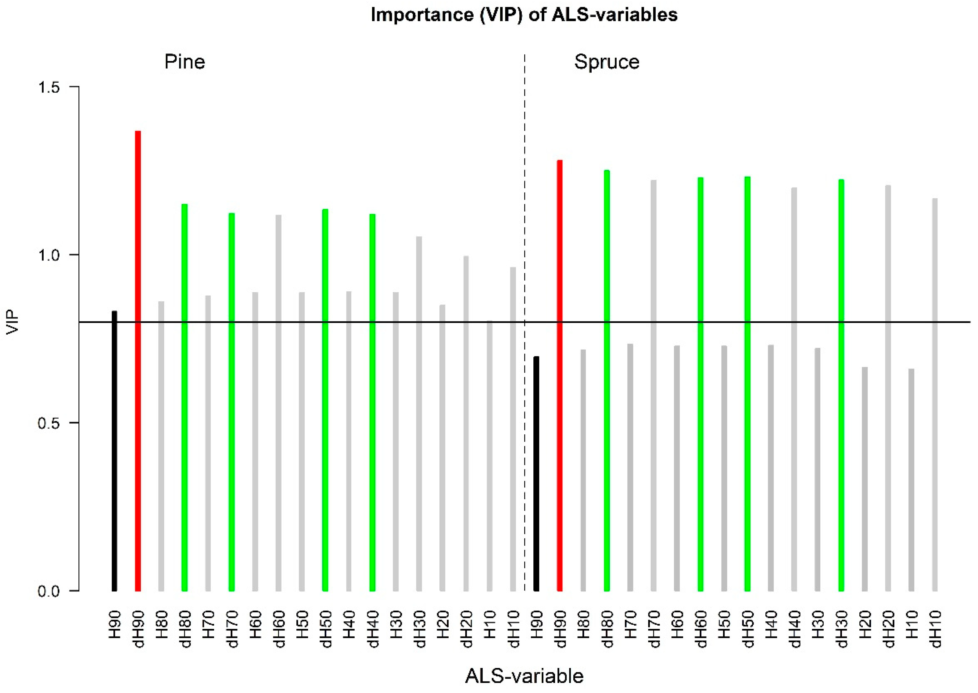
3.1.1. ALS Data

The initial screening of the ALS variables showed that the difference variables scored the highest in terms of VIP, with those from the upper percentiles as the most important ones (dH90 and dH80). Although the VIP scores of the height percentiles were lower compared to those for the difference variables, they were still above the cutoff value of 0.8 for pine-dominated stands. However, for spruce, all VIP scores were lower than the cutoff value. Figure 1 shows the VIP score for both pine and spruce. The five top-ranking variables for each species appear in green. The variables following next on the VIP ranking are indicated with grey bars. The cutoff value is indicated with a horizontal line. Red bars indicate top ranking variables that were selected in the modelling, and black bars indicate variables that were not among the top-ranking ones, but still selected in the final models.

3.1.2. Hyperspectral Data

The results from the screening of the hyperspectral variables and the joint dataset of hyperspectral and ALS variables, are displayed in Figure 2 and Figure 3. The VIP score of the 10 most important variables are displayed with green bars. The other colors have the same interpretation as for Figure 1 (see above). In both Figure 2 and Figure 3, the bars representing ALS variables appear on a yellow background. The results are described in separate sections below.

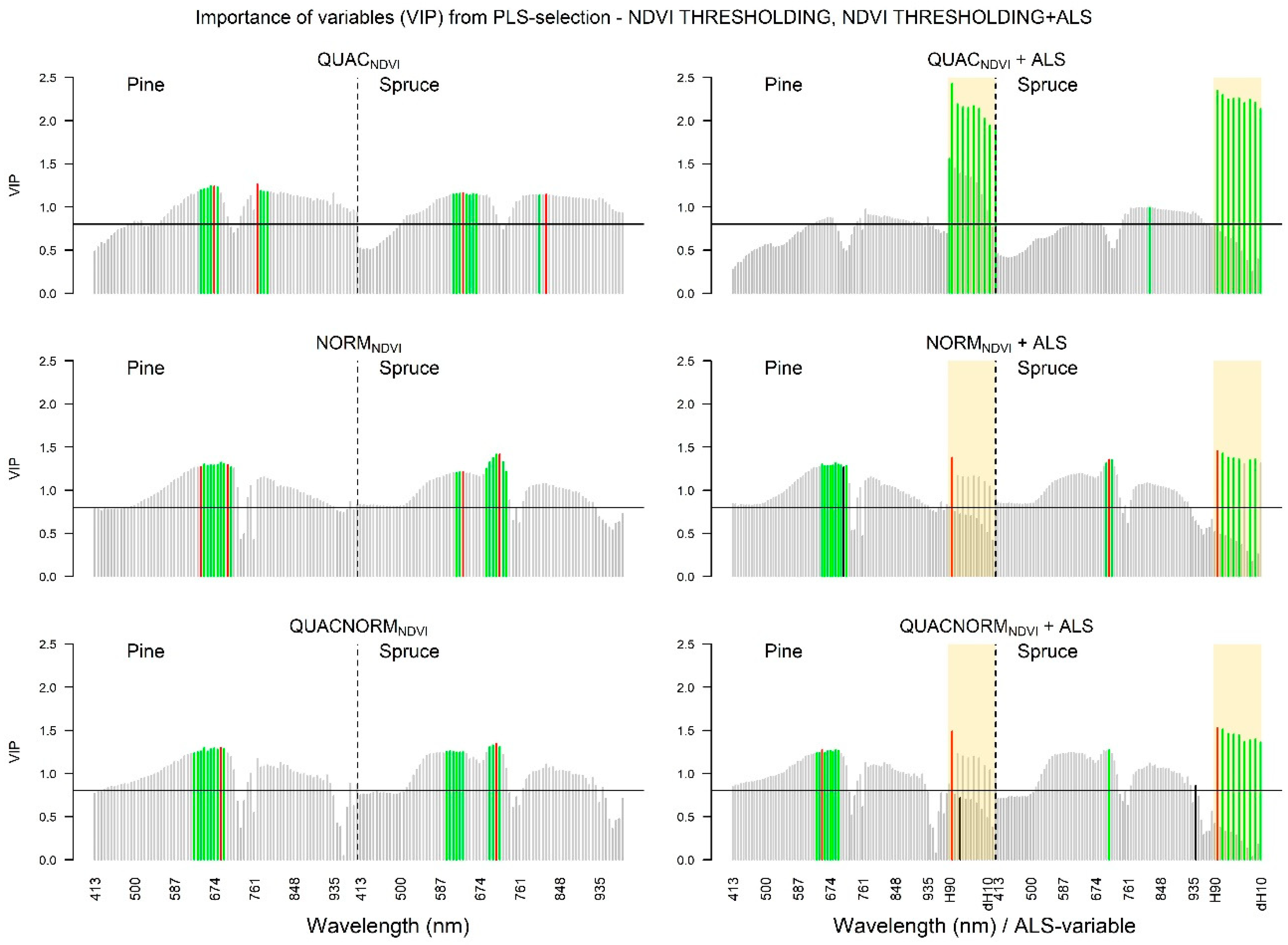
3.1.3. VIP Values: NDVI Selection Threshold

The importance (VIP) of the data using the NDVI threshold in terms of explaining the variation of the H40 site index, seemed to increase to values >0.8 in the interval between 500 nm and 530 nm for both tree species. The most important variables represented wavelengths in the red-edge region, i.e., between 640 nm and 730 nm. These results are displayed graphically in the left column of Figure 2. It can also be seen from the figure that the important spectral bands for spruce were slightly shifted towards longer wavelengths compared to those for pine. The shapes that are formed by the bars in the figure panels also indicate that the type of correction (atmospheric correction, normalization or both) seemed to change the VIP ranking more for spruce compared to pine.

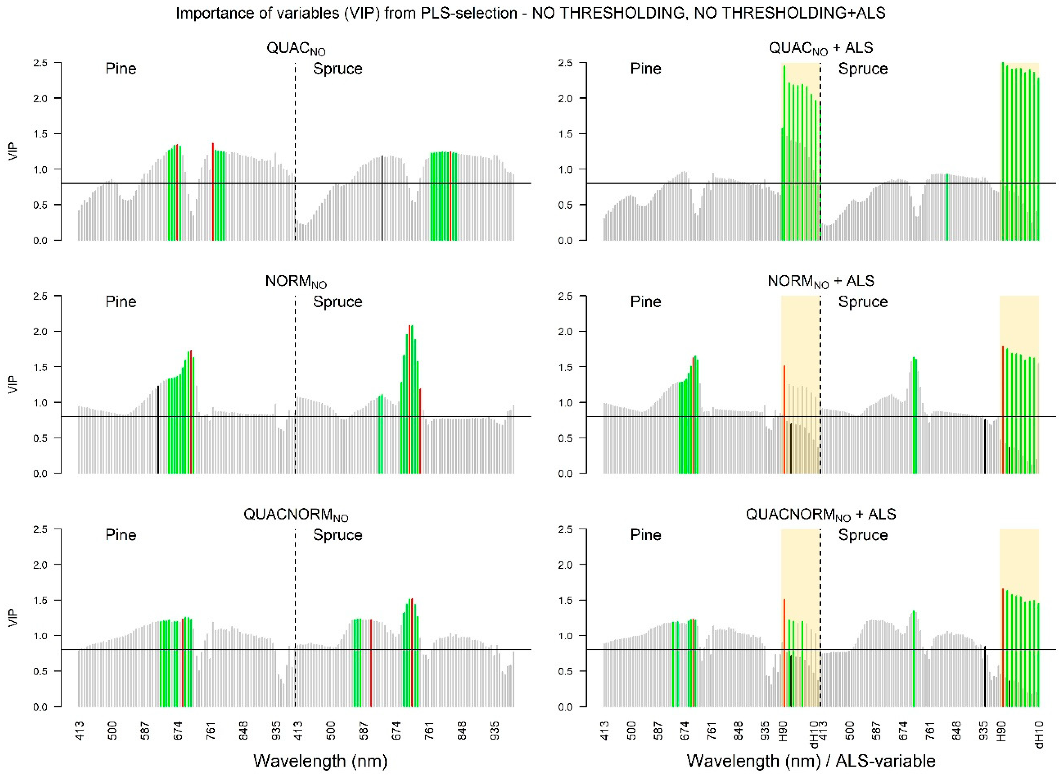
3.1.4. VIP Values: NO Selection Threshold

The importance of the variables calculated from the hyperspectral data, with and without pixel selection threshold (Figure 3), were similar. However, for the QUAC data for spruce (upper left panel), the most important wavelengths were shifted, compared to using NDVI threshold data, to the interval between 770 nm to 830 nm. Furthermore, for the normalized data (middle left panel), the most important variables were the same as the NDVI threshold data, but they were more distinctly differing from the other variables in terms of the VIP value. For both tree species, the most important wavelength was 710 nm. Similar results for the normalized variables were obtained for the QUACNORM variables (lower left panel), although the most important variables did not stand out as distinct, especially not for pine. The most important wavelength for pine was 689 nm and for spruce it was 718 nm.

3.1.5. The Relative Effect of Introducing ALS Data
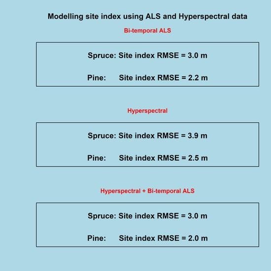
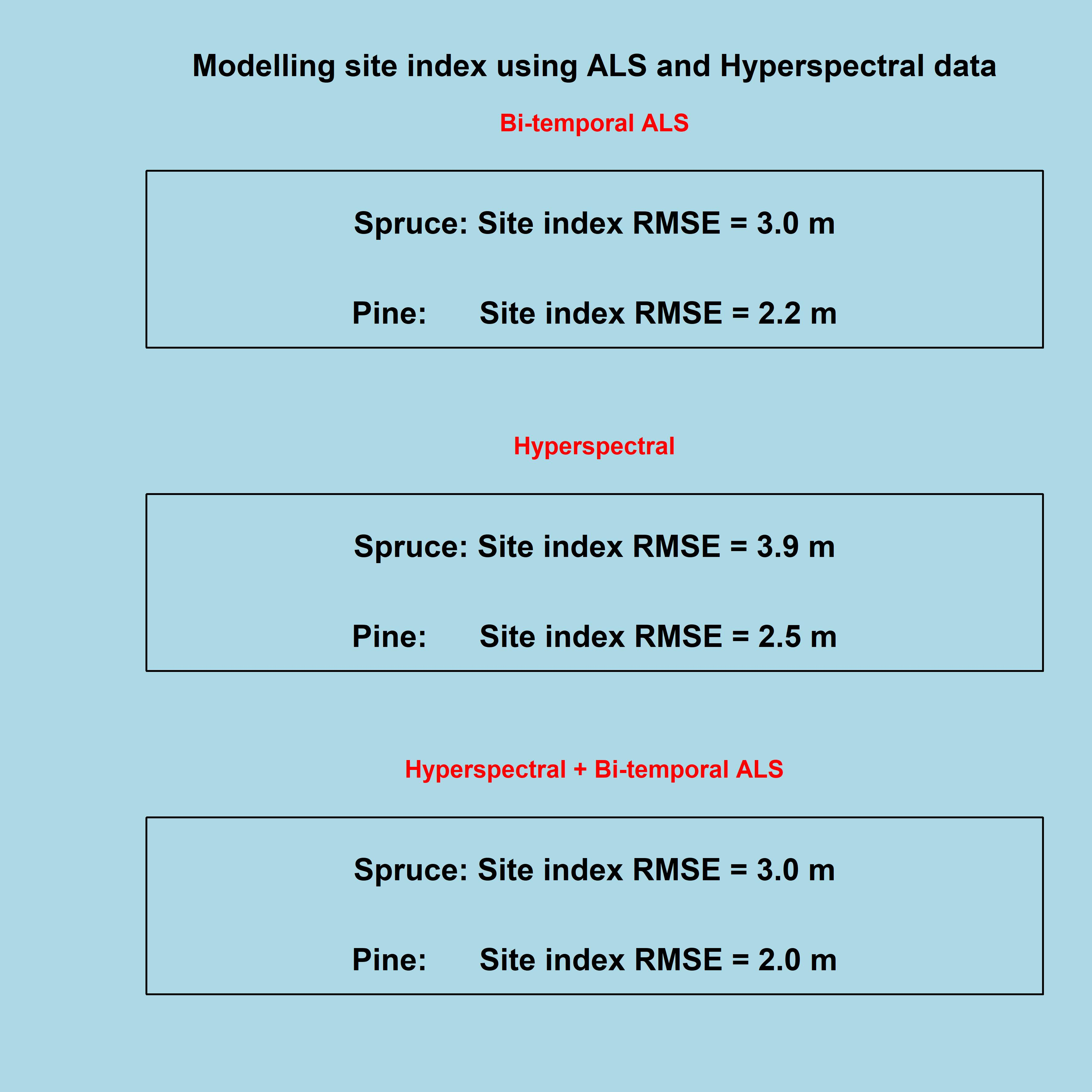
When including also the ALS variables (right columns of Figure 2 and Figure 3) the importance distributions among the hyperspectral variables were more or less maintained. However, the importance of the ALS variables seemed to dominate the QUAC data for both tree species. For the NORM and QUACNORM data, the importance of the hyperspectral variables remained on a high level, but for spruce, eight and nine of the 10 top-ranking variables for NORM and QUACNORM, respectively, were ALS variables.

3.2. Modelling

All the selected variables for the different fitted models (Table 3) were statistically significant (p < 0.05) and the VIF values did not exceed 7.9 for any of them. The modelling revealed no serious problems with regard to non-normality or heteroscedasticity according to the AD and the BP test, respectively, although the BP test indicated heteroscedasticity for one of the models that combined hyperspectral information with ALS (Table 3). For the datasets where models could be fitted with statistically significant parameter estimates, one to three explanatory variables were used. With a couple of exceptions, the final models were fitted using the variables that were ranked as the most important ones after the screening. However, in some cases low-ranking variables had significant contributions to the model judged by RMSE and the distribution of the residuals.

3.2.1. ALS Data

With the ALS data only, the final models included the P901999 and the corresponding difference variable dP90 (Table 3). Although P901999 was not among the five top-ranking variables from the PLSR screening, we considered that a variable representing canopy height at the beginning of the observation period was important to include because a certain height growth over a certain time period is possible for a range of H40 site index values. It is only when the initial height is known that a certain height growth unambiguously can be related to a specific H40 site index value. The cross-validation resulted in RMSE values of 3.04 m and 2.21 m for spruce and pine, respectively.

3.2.2. Hyperspectral Data: NDVI Selection Threshold

The spruce models constructed based on the QUACNDVI data included the variables representing 638 nm and 819 nm wavelengths. This particular inter-distance between wavelengths was wider compared to the one for pine (674 nm and 768 nm). The results are displayed in Table 3, and the selected variables are also indicated by the red bars in the top left panel of Figure 2. The model fit, as expressed by the R2 values, were weaker than for the models comprising only ALS variables, and the cross-validated RMSEs were 4.01 m and 2.49 m for spruce and pine, respectively. The models constructed using variables derived from the NORMNDVI data (Table 3, middle left panel of Figure 2) were more similar between tree species compared to those constructed with the QUACNDVI data. Furthermore, the RMSE values from the cross-validation were slightly smaller using NORMNDVI models, compared to those obtained with QUACNDVI models. The models fitted with the QUACNORMNDVI data were similar to those fitted with NORMNDVI data, but with slightly lower R2, and with only one explanatory variable. With the fused dataset of QUACNDVI and ALS (QUACNDVI + ALS) no model could be fitted while fulfilling the modelling criteria. No combination of variables from QUACNDVI and ALS produced models with statistically significant parameter estimates. However, when ALS variables were combined with NORMNDVI variables, models that included dH90 and a variable representing the 710 nm spectral band could be fitted for both spruce and pine. The model fit and RMSE indicated that the model including ALS variables only, was slightly better for spruce (R2 = 0.70 and RMSE = 3.04 m versus R2 = 0.63 and RMSE = 3.36 m). The results showed the opposite for the pine model, where the NDVI data improved the model slightly. The combination of the QUACNORMNDVI data with the ALS data, however, had a positive effect on the results with higher R2 and smaller RMSE for both tree species. Both models were among the top-ranking models with regard to both R2 and RMSE. The pine model comprised one variable representing the height in 1999 (P701999) and one representing the change in height (dP90), together with the variable representing the 652 nm band. The model for spruce did not include a height variable from ALS but did include a height difference variable (dH90) and the 943 nm band from the QUACNORMNDVI data. The modelling using the combination of single-time ALS and hyperspectral data, failed for all the different hyperspectral datasets. We could not fit any model that fulfilled the criteria.

3.2.3. Hyperspectral Data: NO Selection Threshold

With the QUACNO data, the same variables were selected as for the models constructed with the QUACNDVI data for both tree species, and the R2 values were also similar (Table 3). However, for the models constructed with the NORM data, the selected variables differed between the NDVI threshold and the NO threshold. The spruce model (middle left panel of Figure 3, Table 3) included variables representing 710 nm and 739 nm, and the pine model included variables representing more narrow wavelengths (623 nm and 710 nm). In terms of model fit and cross-validation, the NORM data produced the best model for both tree species on data with NO selection threshold. The R2 of the models constructed with QUACNORMNO data were similar to the NORMNO models, although the selected wavelengths shifted towards the narrow end of the spectrum for spruce, and only one wavelength (689 nm) was selected for pine. The RMSE for the spruce model was 3.80 m with the NORMNO data, 4.04 m with the QUACNO data, and 3.86 m for QUACNORMNO data. The RMSE values were slightly improved when using the NDVI thresholding. As for the NDVI threshold data, no statistically significant variables remained after the modelling the H40 site index with the fused ALS and QUACNO data. With the fused data of NORMNO and ALS, a model with three variables (P701999, dP90, and the NORMNO variable representing 943 nm) was constructed for spruce. Here it can be noted that the NORMNO variable (943 nm) was not among the top-ranking ones, not even among those that were considered to be important, but it was the only one that could be included without violating the criteria of significant variables. The RMSE from the cross-validation was the lowest among the different spruce models (2.88 m). For the pine model, the same ALS variables and the variable representing the spectral wavelength 703 nm were selected. This particular pine model was one of the best of the alternative pine models evaluated by means of the RMSE (1.89 m) and R2 (0.78). The models constructed on the fused ALS and QUACNORMNO data comprised exactly the same variables as the NORMNO + ALS models, and with similar R2 values and cross-validation results. As for the NDVI threshold data with the combination of single-time ALS and hyperspectral data, no significant variables remained after the modelling.

4. Discussion

The analysis showed that among the ALS variables, the difference variables ranked on top in terms of the VIP values (Figure 1). An explanation for this is that relatively long growth periods develop strong relationships between height growth and site index, irrespective of the development stage (initial height). Over a certain number of years, the height growth on the most fertile sites will tend to be greater than on poor sites, even if the trees on the most fertile sites are old and in a slow growing development stage, and the trees on the poor soils are in a fast-growing development stage. The longer the period, the more important the difference variables will be.
The analyses showed that the hyperspectral data fused with ALS data provided only limited additional value, compared to using ALS data only. The main reason is probably that spectral information is mainly related to the species and to the phenological characteristics of the trees, while site index is strongly related to the structural characteristics of forest [63] that is mainly explained by ALS data. Despite this, models dependent only on hyperspectral data obtained R2 values of approximately 0.60. This is very interesting, as it shows that in cases where only spectral data are available, it can still be possible to construct prediction models of the H40 site index. The fact that our results indicate that the site index of pine forest was the most correlated to hyperspectral data, could be explained by that the vegetation on the forest floor differs more between different site indices in pine forest, compared to those of spruce forest along the same gradient. While the vegetation in low-productivity pine forest often is dominated by bare rock and light colored lichens in the Cladonia family, the more productive sites have darker colored heather (Vaccinium family) [64]. Forest density also depends on productivity, so there will be more reflectance from the vegetation on poor sites compared to more productive sites.
Several factors affect the reflectance of trees as registered by hyperspectral sensors, and they have to be considered in the interpretation of the specific results of any study of this kind. There are different spectral signatures for different forest ages [65], and it should be mentioned that in our material there was a strong relationship between age and the H40 site index (r = −0.82, not shown in tables). Moreover, forest vitality will also affect reflectance, so if there is a relationship between H40 site index and the vitality of the forest [66], this could also strengthen the relationship between the hyperspectral variables and H40 site index. The specific time of the acquisition is another factor. The illumination conditions, which are affected by the angle of the sun and shadowing by vegetation and terrain features, may have affected the results even after the atmospheric correction. The phenology, and thereby the reflectance, also naturally change throughout the growth season. There may also be temporal effects of plant stress due to drought, for example, and these factors may vary on small spatial scales. Thus, for the development of prediction models in the context of an FMI, this indicates that it is even more important with the use of hyperspectral data than ALS, to construct models spatially and temporally consistent with the area being inventoried.
It was a surprising result that the normalized data provided models with slightly lower RMSE values compared to the atmospherically corrected data. In the literature, the atmospheric correction is a procedure that is considered essential to the use of hyperspectral data for prediction purposes. However, if the modelling is based on hyperspectral data that are acquired over a short time period, the atmospheric effect among the different stripes could be very small. In the domain of land cover classification, some studies have shown that atmospheric correction is not necessary at all. For instance, in a study by Song et al. [67] it was concluded that atmospheric correction was necessary only when models were applied across spatiotemporal dimensions. Similar conclusions were made in the studies of Kim et al. [68] and Hoffbeck and Landgrebe [69]. Thus, as our study area is small, the normalization could in fact be more useful than to use the atmospheric correction.
All the hyperspectral bands used in the models (Table 3) were in the red and infrared parts of the spectrum. These ranges of the spectrum are generally important for modelling chlorophyll and water content, but also the amount biomass. For example, the bands at 638 and 652 nm can be related to chlorophyll a and b [70]. Moreover, all the selected bands (Table 3) could be used to compute vegetation indices. As an example, the bands 674 and 768 are usually used to compute the narrowband NDVI, or the bands 739 and 718 to the Vogelman index [71]. Vegetation indices are usually used to describe the physiological status of plants.
It was noted that there was a slight difference among the bands selected in the NORM and QUAC datasets. One reason is obviously that the atmospheric correction acts to correct the noisy parts of the spectrum that are usually in the blue- and infrared ranges. Another reason is the data range. The NORM variables have a narrower range compared to the QUAC variables, as the normalization used tends to make the different stripes uniform, and thus remove the slight changes among stripes [53]. The models constructed with QUACNORM data were more similar to NORM models than they were to models constructed with OUAC data. This indicates that the normalization had a more positive effect on the data with regard to improving model fit, compared to the atmospheric correction.
The application of an NDVI threshold for selection of pixels, did not seem to have a pronounced positive effect on the relationship to H40 site index, in contrast to what has been shown in studies on tree species classification [54]. The importance of the highest-ranking variables from the screening even seemed to be more pronounced for the data with NO threshold. The model RMSE, however, were similar for the models using variables computed from hyperspectral data with- and without NDVI threshold in the pixel selection.
Compared to Kandare et al. [22] who used fused ALS and hyperspectral data to predict age and height as input to the appropriate site index curves, our models produced slightly lower RMSE values. At plot level, Kandare et al. [22] obtained an RMSE value of 4.3 m, compared to our range of 1.9–3.4 m with fused hyperspectral and ALS data. Kandare et al. [22] also compared their results to a situation where age was known from field measurements, so that height was the only variable predicted from remotely sensed data. With this combination of data, their RMSE decreased to 1.2 m. Furthermore, Noordermeer at al. [39] used bi-temporal ALS data, where 15 years separated the first and last acquisition. They compared both a direct approach (site index modelled from bi-temporal ALS data) and an indirect approach (site index solved from the site index curves with initial height and change in height as input). At plot level, their cross-validated results showed RMSE values of 2.4 m and 1.9 m for spruce and pine, respectively. This is slightly lower than our results using only ALS variables, but similar to those of our results where hyperspectral variables were included.
In terms of reducing the cost of making in-optimal management decisions because of inaccurate inventory information, site index is one of the most important variables [15]. The study by Eid [15] quantified and reported the loss that could be attributed to random errors in site index, by means of a cost-plus-loss analysis. To determine if the magnitude of reduction in the site index uncertainty as a result of adding hyperspectral information (RMSE: 3.04 m and 2.21 m versus 2.80 m and 1.88 m for spruce and pine, respectively), can defend the acquirement of hyperspectral data in addition to ALS, a similar cost-plus-loss analysis with updated prices and costs have to be carried out.

5. Conclusions

This study has shown that it is possible to model and predict site index using single-time hyperspectral data, but that bi-temporal ALS data explains more of the site index variation. When combining the two data sources, hyperspectral data marginally improved the results compared to only using bi-temporal ALS. In terms of preprocessing of the hyperspectral data, a normalization had greater effect on the data with regard to strengthening the relationship to site index, compared to an atmospheric correction. The selection of pixels based on NDVI did not have a positive effect compared to using all pixels.
There is also a need for more studies on the relationship between hyperspectral information and productivity (site index) in forests. Our dataset only reflects a limited range of forest conditions, and that might have affected the results and conclusions. Site index estimation studies using both bi-temporal ALS and hyperspectral data, should therefore be carried out in a broader range of forest conditions with respect to geographical range, dominant tree species, forest age, and forest productivity.

Author Contributions

The author contributions are as follows: conceptualization, O.M.B., H.O.Ø. and M.D.; methodology, O.M.B., H.O.Ø. and M.D.; validation, O.M.B.; formal analysis, O.M.B.; data curation, H.O.Ø., T.G.; writing—original draft preparation, O.M.B.; writing—review and editing, O.M.B., H.O.Ø., M.D., T.G., E.N.; visualization, O.M.B.; project administration, T.G.; funding acquisition, T.G., E.N.

Funding

This research was funded by Research Council of Norway, grant number 244599.

Acknowledgments

We would like to thank Terratec for collection and preprocessing of the remotely sensed data.

Conflicts of Interest

The authors declare no conflict of interest.

References

  1. Skovsgaard, J.P.; Vanclay, J.K. Forest site productivity: A review of spatial and temporal variability in natural site conditions. For. Int. J. For. Res. 2013, 86, 305–315. [Google Scholar] [CrossRef]
  2. Pretzsch, H.; Grote, R.; Reineking, B.; Rötzer, T.; Seifert, S. Models for forest ecosystem management: A european perspective. Ann. Bot. 2008, 101, 1065–1087. [Google Scholar] [CrossRef] [PubMed]
  3. Rivas, J.J.C.; González, J.G.Á.; Aguirre, O.; Hernández, F.J. The effect of competition on individual tree basal area growth in mature stands of pinus cooperi blanco in durango (mexico). Eur. J. For. Res. 2005, 124, 133–142. [Google Scholar] [CrossRef]
  4. Bollandsås, O.M.; Næsset, E. Weibull models for single-tree increment of norway spruce, scots pine, birch and other broadleaves in norway. Scand. J. For. Res. 2009, 24, 54–66. [Google Scholar] [CrossRef]
  5. Hasenauer, H.; Monserud, R.A. Biased predictions for tree height increment models developed from smoothed ‘data’. Ecol. Model. 1997, 98, 13–22. [Google Scholar] [CrossRef]
  6. Hasenauer, H.; Monserud, R.A.; Gregoire, T.G. Using simultaneous regression techniques with individual-tree growth models. For. Sci. 1998, 44, 87–95. [Google Scholar]
  7. Sharma, R.P.; Brunner, A. Modeling individual tree height growth of norway spruce and scots pine from national forest inventory data in norway. Scand. J. For. Res. 2017, 32, 501–514. [Google Scholar] [CrossRef]
  8. Sharma, R.P.; Brunner, A.; Eid, T.; Øyen, B.-H. Modelling dominant height growth from national forest inventory individual tree data with short time series and large age errors. For. Ecol. Manag. 2011, 262, 2162–2175. [Google Scholar] [CrossRef]
  9. Pienaar, L.V.; Rheney, J.W. Modeling stand level growth and yield response to silvicultural treatments. For. Sci. 1995, 41, 629–638. [Google Scholar]
  10. Boisvenue, C.; Running, S.W. Impacts of climate change on natural forest productivity—Evidence since the middle of the 20th century. Glob. Chang. Biol. 2006, 12, 862–882. [Google Scholar] [CrossRef]
  11. Sharma, R.P.; Brunner, A.; Eid, T. Site index prediction from site and climate variables for norway spruce and scots pine in norway. Scand. J. For. Res. 2012, 27, 619–636. [Google Scholar] [CrossRef]
  12. Skovsgaard, J.P.; Vanclay, J.K. Forest site productivity: A review of the evolution of dendrometric concepts for even-aged stands. For. Int. J. For. Res. 2008, 81, 13–31. [Google Scholar] [CrossRef]
  13. Tveite, B. Bonitetskurver for Gran; Norsk Institutt for Skogforskning: Ås, Norway, 1977; pp. 1–84. [Google Scholar]
  14. Tveite, B.; Braastad, H. Bonitering for gran, furu og bjørk. Nor. Skogbr. 1981, 27, 17–22. [Google Scholar]
  15. Eid, T. Use of uncertain inventory data in forestry scenario models and consequential incorrect harvest decisions. Silva Fenn. 2000, 34, 89–100. [Google Scholar] [CrossRef]
  16. Næsset, E. Predicting forest stand characteristics with airborne scanning laser using a practical two-stage procedure and field data. Remote Sens. Environ. 2002, 80, 88–99. [Google Scholar] [CrossRef]
  17. Næsset, E. Area-based inventory in norway—From innovation to an operational reality. In Forestry Applications of Airborne Laser Scanning: Concepts and Case Studies; Maltamo, M., Næsset, E., Vauhkonen, J., Eds.; Springer: Dordrecht, The Netherlands, 2014; pp. 215–240. [Google Scholar]
  18. Gatziolis, D.; Fried, J.S.; Monleon, V.S. Challenges to estimating tree height via lidar in closed-canopy forests: A parable from western oregon. For. Sci. 2010, 56, 139–155. [Google Scholar]
  19. Packalén, P.; Mehtätalo, L.; Maltamo, M. Als-based estimation of plot volume and site index in a eucalyptus plantation with a nonlinear mixed-effect model that accounts for the clone effect. Ann. For. Sci. 2011, 68, 1085. [Google Scholar] [CrossRef]
  20. Chen, Y.; Zhu, X. Site quality assessment of a pinus radiata plantation in victoria, australia, using lidar technology. South. For. J. For. Sci. 2012, 74, 217–227. [Google Scholar] [CrossRef]
  21. Tompalski, P.; Coops, N.C.; White, J.C.; Wulder, M.A.; Pickell, P.D. Estimating forest site productivity using airborne laser scanning data and landsat time series. Can. J. Remote Sens. 2015, 41, 232–245. [Google Scholar] [CrossRef]
  22. Kandare, K.; Ørka, H.O.; Dalponte, M.; Næsset, E.; Gobakken, T. Individual tree crown approach for predicting site index in boreal forests using airborne laser scanning and hyperspectral data. Int. J. Appl. Earth Obs. Geoinf. 2017, 60, 72–82. [Google Scholar] [CrossRef]
  23. Holopainen, M.; Vastaranta, M.; Yu, X.; Haapanen, R.; Hyyppä, J.; Kaartinen, H.; Viitala, R.; Hyyppä, H. Site type estimation using airborne laser scanning and stand register data. Photogramm. J. Finl. 2010, 22, 16–32. [Google Scholar]
  24. Vehmas, M.; Eerikäinen, K.; Peuhkurinen, J.; Packalén, P.; Maltamo, M. Airborne laser scanning for the site type identification of mature boreal forest stands. Remote Sens. 2011, 3, 100–116. [Google Scholar] [CrossRef]
  25. Næsset, E. Practical large-scale forest stand inventory using a small-footprint airborne scanning laser. Scand. J. For. Res. 2004, 19, 164–179. [Google Scholar] [CrossRef]
  26. Eid, T. Standwise Control of Forest Management Planning Data in Cutting Class III–V; Meddelelser fra Skogforskningen: Ås, Norway, 1992; pp. 1–78. [Google Scholar]
  27. Eid, T. Kontroll av Skogbruksplandata fra “Understøttet Fototakst”; Aktuelt fra Skogforsk: Ås, Norway, 1996; pp. 1–21. [Google Scholar]
  28. Eid, T.; Nersten, S. Sammenligning av skogbruksplandata og kontrolldata. In Problemer Omkring Registreringer og Planlegging for en Skogeiendom i Birkenes Kommune; Eid, T., Ed.; Skogforsk: Ås, Norway, 1996; Volume 47, pp. 1–34. [Google Scholar]
  29. St-Onge, B.; Vepakomma, U. Assessing forest gap dynamics and growth using multi-temporal laser-scanner data. Int. Arch. Photogramm. Remote Sens. Spat. Inf. Sci. 2004, 140, 173–178. [Google Scholar]
  30. Bollandsås, O.M.; Gregoire, T.G.; Næsset, E.; Øyen, B.-H. Detection of biomass change in a norwegian mountain forest area using small footprint airborne laser scanner data. Stat. Methods Appl. 2013, 22, 113–129. [Google Scholar] [CrossRef]
  31. Ene, L.T.; Næsset, E.; Gobakken, T.; Bollandsås, O.M.; Mauya, E.W.; Zahabu, E. Large-scale estimation of change in aboveground biomass in miombo woodlands using airborne laser scanning and national forest inventory data. Remote Sens. Environ. 2017, 188, 106–117. [Google Scholar] [CrossRef]
  32. Næsset, E.; Bollandsås, O.M.; Gobakken, T.; Gregoire, T.G.; Ståhl, G. Model-assisted estimation of change in forest biomass over an 11year period in a sample survey supported by airborne lidar: A case study with post-stratification to provide “activity data”. Remote Sens. Environ. 2013, 128, 299–314. [Google Scholar] [CrossRef]
  33. Strîmbu, V.F.; Ene, L.T.; Gobakken, T.; Gregoire, T.G.; Astrup, R.; Næsset, E. Post-stratified change estimation for large-area forest biomass using repeated als strip sampling. Can. J. For. Res. 2017, 47, 839–847. [Google Scholar] [CrossRef]
  34. Hyyppä, J.; Yu, X.; Rönnholm, P.; Kaartinen, H.; Hyyppä, H. Factors affecting laser-derived object-oriented forest height growth estimation. Photogramm. J. Finl. 2003, 18, 16–31. [Google Scholar]
  35. Næsset, E.; Gobakken, T. Estimating forest growth using canopy metrics derived from airborne laser scanner data. Remote Sens. Environ. 2005, 96, 453–465. [Google Scholar] [CrossRef]
  36. Hollaus, M.; Eysn, L.; Maier, B.; Pfeifer, N. Site index assessment based on multi-temporal als data. In Proceedings of the Silvilaser 2015, La Grande Motte, France, 28–30 September 2015. [Google Scholar]
  37. Kvaalen, H.; Solberg, S.; May, J. Aldersuavhengig Bonitering Med Laserscanning av Enkelttrær; Rapport fra NIBIO: Ås, Norway, 2015; pp. 1–31. [Google Scholar]
  38. Gobakken, T.; Næsset, E. Assessing effects of laser point density, ground sampling intensity, and field sample plot size on biophysical stand properties derived from airborne laser scanner data. Can. J. For. Res. 2008, 38, 1095–1109. [Google Scholar] [CrossRef]
  39. Noordermeer, L.; Bollandsås, O.M.; Gobakken, T.; Næsset, E. Direct and indirect site index determination for norway spruce and scots pine using bitemporal airborne laser scanner data. For. Ecol. Manag. 2018, 428, 104–114. [Google Scholar] [CrossRef]
  40. Baltsavias, E.; Gruen, A.; Eisenbeiss, H.; Zhang, L.; Waser, L.T. High-quality image matching and automated generation of 3d tree models. Int. J. Remote Sens. 2008, 29, 1243–1259. [Google Scholar] [CrossRef]
  41. Véga, C.; St-Onge, B. Mapping site index and age by linking a time series of canopy height models with growth curves. For. Ecol. Manag. 2009, 257, 951–959. [Google Scholar] [CrossRef]
  42. Dalponte, M.; Bruzzone, L.; Gianelle, D. Tree species classification in the southern alps based on the fusion of very high geometrical resolution multispectral/hyperspectral images and lidar data. Remote Sens. Environ. 2012, 123, 258–270. [Google Scholar] [CrossRef]
  43. Ørka, H.O.; Dalponte, M.; Gobakken, T.; Næsset, E.; Ene, L.T. Characterizing forest species composition using multiple remote sensing data sources and inventory approaches. Scand. J. For. Res. 2013, 28, 677–688. [Google Scholar] [CrossRef]
  44. Smith, M.; Martin, M.E.; Plourde, L.; Ollinger, S.V. Analysis of hyperspectral data for estimation of temperate forest canopy nitrogen concentration: Comparison between an airborne (aviris) and a spaceborne (hyperion) sensor. IEEE Trans. Geosci. Remote Sens. 2003, 41, 1332–1337. [Google Scholar] [CrossRef]
  45. Smith, M.-L.; Ollinger, S.V.; Martin, M.E.; Aber, J.D.; Hallett, R.A.; Goodale, C.L. Direct estimation of aboveground forest productivity through hyperspectral remote sensing of canopy nitrogen. Ecol. Appl. 2002, 12, 1286–1302. [Google Scholar] [CrossRef]
  46. Eid, T.; Tuhus, E. Models for individual tree mortality in norway. For. Ecol. Manag. 2001, 154, 69–84. [Google Scholar] [CrossRef]
  47. Næsset, E. Determination of mean tree height of forest stands by digital photogrammetry. Scand. J. For. Res. 2002, 17, 446–459. [Google Scholar] [CrossRef]
  48. Anon. Terrascan User’s Guide; Terrasolid Ltd.: Jyvaskyla, Finland, 2016. [Google Scholar]
  49. Axelsson, P. Dem generation from laser scanner data using adaptive tin models. Int. Arch. Photogramm. Remote Sens. 2000, 33, 110–117. [Google Scholar]
  50. Cao, F.; Yang, Z.; Ren, J.; Jiang, M.; Ling, W.-K. Does Normalization Methods Play a Role for Hyperspectral Image Classification? 2017. Available online: https://arxiv.org/abs/1710.02939 (accessed on 29 April 2019).
  51. Bernstein, L.S.; Adler-Golden, S.M.; Sundberg, R.L.; Levine, R.Y.; Perkins, T.C.; Berk, A.; Ratkowski, A.J.; Felde, G.; Hoke, M.L. A new method for atmospheric correction and aerosol optical property retrieval for vis-swir multi- and hyperspectral imaging sensors: Quac (quick atmospheric correction). In Proceedings of the 2005 IEEE International Geoscience and Remote Sensing Symposium, IGARSS ’05, Seoul, Korea, 29 July 2005; pp. 3549–3552. [Google Scholar]
  52. Rani, N.; Mandla, V.R.; Singh, T. Evaluation of atmospheric corrections on hyperspectral data with special reference to mineral mapping. Geosci. Front. 2017, 8, 797–808. [Google Scholar] [CrossRef]
  53. Yu, B.; Ostland, M.; Gong, P.; Pu, R. Penalized discriminant analysis of in situ hyperspectral data for conifer species recognition. IEEE Trans. Geosci. Remote Sens. 1999, 37, 2569–2577. [Google Scholar] [CrossRef]
  54. Dalponte, M.; Ørka, H.O.; Ene, L.T.; Gobakken, T.; Næsset, E. Tree crown delineation and tree species classification in boreal forests using hyperspectral and als data. Remote Sens. Environ. 2014, 140, 306–317. [Google Scholar] [CrossRef]
  55. Martens, H.; Martens, M. Multivariate Analysis of Quality: An Introduction; John Wiley & Sons: Hoboken, NJ, USA, 2000. [Google Scholar]
  56. Wold, S.; Sjöström, M.; Eriksson, L. Pls-regression: A basic tool of chemometrics. Chemom. Intell. Lab. Syst. 2001, 58, 109–130. [Google Scholar] [CrossRef]
  57. Wold, S. Pls for multivariate linear modeling. In Chemometric Methods in Molecular Design; Waterbeemd, H.V.D., Ed.; VCH Verlagsgesellschaft mbH: Weinheim, Germany, 1994; pp. 195–218. [Google Scholar]
  58. McRoberts, R.E.; Næsset, E.; Gobakken, T.; Bollandsås, O.M. Indirect and direct estimation of forest biomass change using forest inventory and airborne laser scanning data. Remote Sens. Environ. 2015, 164, 36–42. [Google Scholar] [CrossRef]
  59. Anon. Sas® 9.4 Statements: Reference; SAS Institute Inc.: Cary, NC, USA, 2016. [Google Scholar]
  60. Montgomery, D.; Peck, E.; Vining, G. Introduction to Linear Regression Analysis; John Wiley & Sons, Inc.: Hoboken, NJ, USA, 2013. [Google Scholar]
  61. Stephens, M.A. Edf statistics for goodness of fit and some comparisons. J. Am. Stat. Assoc. 1974, 69, 730–737. [Google Scholar] [CrossRef]
  62. Breusch, T.S.; Pagan, A.R. A simple test for heteroscedasticity and random coefficient variation. Econometrica 1979, 47, 1287–1294. [Google Scholar] [CrossRef]
  63. Bolton, D.K.; Coops, N.C.; Wulder, M.A. Measuring forest structure along productivity gradients in the canadian boreal with small-footprint lidar. Environ. Monit. Assess. 2013, 185, 6617–6634. [Google Scholar] [CrossRef]
  64. Fremstad, E. Vegetasjonstyper i Norge; Norsk Institutt for Naturforskning: Trondheim, Norway, 1997; pp. 1–279. [Google Scholar]
  65. Rautiainen, M.; Lukeš, P.; Homolová, L.; Hovi, A.; Pisek, J.; Mõttus, M. Spectral properties of coniferous forests: A review of in situ and laboratory measurements. Remote Sens. 2018, 10, 207. [Google Scholar] [CrossRef]
  66. Reichmuth, A.; Henning, L.; Pinnel, N.; Bachmann, M.; Rogge, D. Early detection of vitality changes of multi-temporal norway spruce laboratory needle measurements—The ring-barking experiment. Remote Sens. 2018, 10, 57. [Google Scholar] [CrossRef]
  67. Song, C.; Woodcock, C.E.; Seto, K.C.; Lenney, M.P.; Macomber, S.A. Classification and change detection using landsat tm data: When and how to correct atmospheric effects? Remote Sens. Environ. 2001, 75, 230–244. [Google Scholar] [CrossRef]
  68. Kim, S.-H.; Shin, J.-I.; Yoo, H.-R.; Lee, K.-S. Effect of Atmospheric Correction for the Land Cover Classification Using Hyperspectral Data. Proceedings of Asian Association on Remote Sensing—27th Asian Conference on Remote Sensing, ACRS 2006, Ulaanbaatar, Mongolia, 9–13 October 2006. [Google Scholar]
  69. Hoffbeck, J.P.; Landgrebe, D.A. Effect of radiance-to-reflectance transformation and atmosphere removal on maximum likelihood classification accuracy of high-dimensional remote sensing data. In Surface and Atmospheric Remote Sensing: Technologies, Data Analysis and Interpretation, Proceedings of the Geoscience and Remote Sensing Symposium (IGARSS ’94), Pasadena, CA, USA, 8–12 August 1994; IEEE: New York, NY, USA, 1994; Volume 4, pp. 2538–2540. [Google Scholar]
  70. Siebke, K.; Ball, M.C. Non-destructive measurement of chlorophyll b:A ratios and identification of photosynthetic pathways in grasses by reflectance spectroscopy. Funct. Plant Biol. 2009, 36, 857–866. [Google Scholar] [CrossRef]
  71. Agapiou, A.; Hadjimitsis, D.G.; Alexakis, D.D. Evaluation of broadband and narrowband vegetation indices for the identification of archaeological crop marks. Remote Sens. 2012, 4, 3892. [Google Scholar] [CrossRef]
Figure 1. Variable importance for projection (VIP) values from the partial least squares (PLS) analysis with site index as a response for ALS-variables. Results for pine appear on the left, and results for spruce appear on the right. The five top-ranking variables according to VIP appear in green. Variables among the top-ranking variables that were included in the subsequent modelling appear in red. Black bars indicate variables that were selected in the modelling, but that were not among the top five.
Remotesensing 11 01020 g001
Figure 2. Variable importance for projection (VIP) values from the partial least squares (PLS) analysis with site index as a response for hyperspectral variables, and hyperspectral variables in combination with ALS variables. In each panel, results for pine appear on the left, and results for spruce appear on the right. The 10 top-ranking variables according to VIP appear in green. Variables among the top-ranking variables that were included in the subsequent modelling appear in red. Black bars indicate variables that were selected in the modelling, but that were not among the top 10. The results in each panel show variables derived from hyperspectral data where pixels were selected with a NDVI threshold but with different preprocessing; upper left: atmospherically corrected hyperspectral data; middle left: normalized hyperspectral data; lower left: atmospherically corrected and normalized hyperspectral data; upper right: atmospherically corrected hyperspectral data with ALS variables; middle right: normalized hyperspectral data with ALS variables; lower right: atmospherically corrected and normalized hyperspectral data with ALS variables. In the right column of the panels, the bars representing the ALS variables appear on a yellow background. The sequence of ALS variables from left to right is H901999, dH90, H801999, dH80, …, H101999, and dH10.
Remotesensing 11 01020 g002
Figure 3. Variable importance for projection (VIP) values from partial least squares (PLS) analysis with site index as a response for hyperspectral variables, and hyperspectral variables in combination with ALS variables. In each panel, results for pine appear on the left, and results for spruce appear on the right. The 10 top-ranking variables according to VIP appear in green. Variables among the top-ranking variables that were included in the subsequent modelling appear in red. Black bars indicate variables that were selected in the modelling, but that were not among the top 10. The results in each panel show variables derived from hyperspectral data where pixels were selected without any thresholding, but with different preprocessing; upper left: atmospherically corrected hyperspectral data; middle left: normalized hyperspectral data; lower left: atmospherically corrected and normalized hyperspectral data; upper right: atmospherically corrected hyperspectral data with ALS variables; middle right: normalized hyperspectral data with ALS variables; lower right: atmospherically corrected and normalized hyperspectral data with ALS variables. In the right column of the panels, the bars representing the ALS variables appear on a yellow background. The sequence of ALS variables from left to right is H901999, dH90, H801999, dH80, …, H101999, and dH10.
Remotesensing 11 01020 g003
Table 1. Mean values and ranges of field-observed variables in 1999, 2010, and 2013.
Variable1999 (n = 65 *)2010 (n = 81)2013 (n = 81)
SprucePROP0.45 (0.0–1.0)0.51 (0.0–1.0)
PinePROP0.43 (0.0–1.0)0.40 (0.0–1.0)
DecidPROP0.11 (0.0–0.5)0.09 (0.0–0.4)
N (ha−1)1624 (350–4600) 1686 (350–5700)
HDOM (m)18.1 (8.3–28.8)20.4 (13.6–30.6)20.0 (11.8–30.4)
Stand age (yrs) 85 (24–209)
H40 site index (m) 14.5 (6.2–25.8)
SprucePROP = volume proportion of spruce; PinePROP = volume proportion of pine; DecidPROP = volume proportion of deciduous species; N = number of stems; HDOM = dominant height: the average height of the 100 largest trees according to diameter per hectare. * 16 plots were defined as regeneration plots in 1999, and thus, registered according to a different field protocol than the mature plots.
Table 2. Parameters for ALS campaigns in 1999 and 2011.
Parameter19992011
Dates8–9 June9 September
InstrumentOptech ALTM 1210Leica ALS70
Average flying altitude (m above ground level)7001500
Flight speed (ms−1)7170
Pulse repetition frequency (kHz)10181
Scan frequency (Hz)21.037.7
Half scan angle (degrees)14.020
Pulse density on the ground (m−2)1.22.4
Table 3. Results from modelling the H40 site index using variables derived from either bi-temporal ALS data, hyperspectral data, or a combination of the two.
ModelDominant SpeciesExplanatory VariablesAD TestBP TestR2RMSE
(m)
VIF
ALSSpruceP901999 dP90nsns0.703.041.7
PineP901999 dP90nsns0.692.213.0
QUACNDVISpruce638 nm, 819 nmnsns0.484.012.1
Pine674 nm, 768 nmnsns0.592.492.3
NORMNDVISpruce638 nm, 718 nmnsns0.543.782.6
Pine645 nm, 703 nmnsns0.602.437.9
QUACNORMNDVISpruce710 nmnsns0.473.931
Pine689 nmnsns0.562.481
QUACNDVI + ALSSpruce- --
Pine- --
NORMNDVI + ALSSprucedP90, 710 nmnsns0.633.362.4
PinedP90, 710 nmns*0.712.141.9
QUACNORMNDVI + ALSSprucedP90, 943 nmnsns0.752.801
PineP701999, dP90, 652 nmnsns0.771.884.6
QUACNOSpruce638 nm, 819 nmnsns0.474.042.0
Pine674 nm, 768 nmnsns0.562.591.9
NORMNOSpruce710 nm, 739 nmnsns0.523.801.2
Pine623 nm, 710 nmnsns0.602.431.3
QUACNORMNOSpruce609 nm, 718 nmnsns0.513.861.7
Pine689 nmnsns0.532.571
QUACNO + ALSSpruce- --
Pine- --
NORMNO + ALSSpruceP701999 dP90, 943 nmnsns0.752.881.8
PineP701999 dP90, 703 nmnsns0.781.894.0
QUACNORMNO + ALSSpruceP701999 dP90, 943 nmnsns0.762.862.6
PineP701999 dP90, 703 nmnsns0.751.914.1
AD test = Anderson–Darling test of normality; BP test = Breush–Pagan test of heteroscedasticity; R2 = coefficient of determination; RMSE = root mean square error from leave-one-out cross-validation; VIF = maximum variance inflation factor.

