Article

Estimating Daily PM2.5 Concentrations in Beijing Using 750-M VIIRS IP AOD Retrievals and a Nested Spatiotemporal Statistical Model

1
Key Laboratory for Urban Habitat Environmental Science and Technology, Shenzhen Graduate School, Peking University, Shenzhen 518055, China
2
School of GeoSciences, University of Edinburgh, Edinburgh EH8 9YL, UK
3
Laboratory for Earth Surface Processes, Ministry of Education, College of Urban and Environmental Sciences, Peking University, Beijing 100871, China
4
Department of Urban Planning and Design, The University of Hong Kong, Hong Kong SAR, China
5
Shenzhen Institute of Research and Innovation, The University of Hong Kong, Shenzhen 518075, China
*
Author to whom correspondence should be addressed.
Remote Sens. 2019, 11(7), 841; https://doi.org/10.3390/rs11070841
Submission received: 6 January 2019 / Revised: 2 April 2019 / Accepted: 4 April 2019 / Published: 8 April 2019
(This article belongs to the Section Atmospheric Remote Sensing)

Abstract

:
Satellite-retrieved aerosol optical depth (AOD) data have been widely used to predict PM2.5 concentrations. Most of their spatial resolutions (~1 km or greater), however, are too coarse to support PM2.5-related studies at fine scales (e.g., urban-scale PM2.5 exposure assessments). Space-time regression models have been widely developed and applied to predict PM2.5 concentrations from satellite-retrieved AOD. Their accuracies, however, are not satisfactory particularly on days that lack a model dataset. The present study aimed to evaluate the effectiveness of recent high-resolution (i.e., ~750 m at nadir) AOD obtained from the Visible Infrared Imaging Radiometer Suite instrument (VIIRS) Intermediate Product (IP) in estimating PM2.5 concentrations with a newly developed nested spatiotemporal statistical model. The nested spatiotemporal statistical model consisted of two parts: a nested time fixed effects regression (TFER) model and a series of geographically weighted regression (GWR) models. The TFER model, containing daily, weekly, or monthly intercepts, used the VIIRS IP AOD as the main predictor alongside several auxiliary variables to predict daily PM2.5 concentrations. Meanwhile, the series of GWR models used the VIIRS IP AOD as the independent variable to correct residuals from the first-stage nested TFER model. The average spatiotemporal coverage of the VIIRS IP AOD was approximately 16.12%. The sample-based ten-fold cross validation goodness of fit (R2) for the first-stage TFER models with daily, weekly, and monthly intercepts were 0.81, 0.66, and 0.45, respectively. The second-stage GWR models further captured the spatial heterogeneities of the PM2.5-AOD relationships. The nested spatiotemporal statistical model produced more daily PM2.5 estimates and improved the accuracies of summer, autumn, and annual PM2.5 estimates. This study contributes to the knowledge of how well VIIRS IP AOD can predict PM2.5 concentrations at urban scales and offers strategies for improving the coverage and accuracy of daily PM2.5 estimates on days that lack a model dataset.

Graphical Abstract

1. Introduction

PM2.5 (fine particles with an aerodynamic diameter ≤ 2.5 μm) produced by both natural and anthropogenic sources [1] is one of the main causes of ambient air pollution, which is thought to lead to approximately 3.3 million deaths per year worldwide [2,3]. Cities within China, India, and other developing countries have some of the highest levels of mortality/morbidity associated with PM2.5 due to the effects of atmospheric transport and international trade [4]. PM2.5 also influences atmospheric visibility and climate change [5]. To avoid the negative effects of PM2.5, a series of laws, regulations, and standards have been implemented in various countries [6]. The determination of ground-level PM2.5 concentrations with high accuracy, resolution, and coverage, either from measuring or modeling [7,8], is critical for accurate assessment of both PM2.5-related effects and policy measures. Inferring ground-level PM2.5 concentrations from satellite-retrieved aerosol optical depth (AOD) data is an effective tool that can partially fill the monitoring gap left by ground monitors, which has led to its increase in popularity for predicting PM2.5 concentrations [9,10,11] and PM2.5-related health effects [12,13].
A handful of satellite-retrieved AOD are available to predict PM2.5 concentrations. These can be divided into fine-resolution (i.e., <10 km) and coarse-resolution (i.e., ≥10 km) AOD according to their spatial resolutions [14]. Fine-resolution AOD can reveal more spatial details on PM2.5 pollution than coarse-resolution AOD, benefitting urban-scale epidemiological studies. Existing fine-resolution AOD mainly include 3-km MODIS (Moderate Resolution Imaging Spectroradiometer) AOD [15,16], 750-m/6-km VIIRS (Visible Infrared Imaging Radiometer Suite) AOD [17,18], 1-km MAIAC (Multi-Angle Implementation of Atmospheric Correction) AOD [19,20], and 160-m GF (Gaofen) AOD [21]. The 750-m VIIRS IP (Intermediate Product) AOD has the highest spatial resolution (better than 1 km) among those that can be directly accessed and downloaded. Its accuracy has been evaluated on urban [22], regional [23], and national scales [24]. Although the VIIRS IP AOD was somewhat inferior to that of MODIS or GOCI (Geostationary Ocean Color Imager) in terms of accuracy, a good proportion of the VIIRS IP AOD retrievals fell within the reference expected error envelope (e.g., 33% in Beijing from 2012 to 2013 [23]). With this profile, the VIIRS IP AOD is believed to have the potential to benefit exposure studies at fine scales because of its high spatial resolution [22,23,24]. Although it has been successfully used to depict the temporal and spatial pattern of AOD in China [24], its potential for directly estimating PM2.5 concentrations has been tested only on a limited basis.
Geophysical models [25,26], statistical models, and machine learning models [27,28,29] are the three main approaches to predicting PM2.5 concentrations from satellite-retrieved AOD. Compared with geophysical and machine learning models, statistical models are simpler and can produce PM2.5 estimates with relatively high accuracy. As a result, statistical models have experienced rapid development, evolving from simple linear regression models [30], in earlier times, to the present advanced statistical models. Representatives of advanced statistical models include linear mixed effects models, which allow temporal heterogeneities [31], geographically weighted regression (GWR) models, which capture spatial heterogeneities [32,33], and space-time regression models, which consider spatiotemporal heterogeneities [34,35]. Statistical models, however, require ground monitored PM2.5 data to perform model calibration and validation. Consequently, it is still hard to obtain satisfactory PM2.5 estimates for those areas or days that lack a model dataset.
The present study aimed to evaluate the effectiveness of the 750-m VIIRS AOD in estimating PM2.5 concentrations with a newly developed nested spatiotemporal statistical model. The model enabled spatiotemporal heterogeneities of PM2.5-AOD relationships to be captured and aimed to improve the coverage and accuracy of PM2.5 estimates for days without a model dataset. The rest of the paper is organized as follows. Data sources and model development and validation procedures are described in the Data and Methods section. The Results and Discussion section provides a description of model performance, PM2.5 estimates, and associated uncertainties. Conclusions are presented at the end of the paper.

2. Materials and Methods

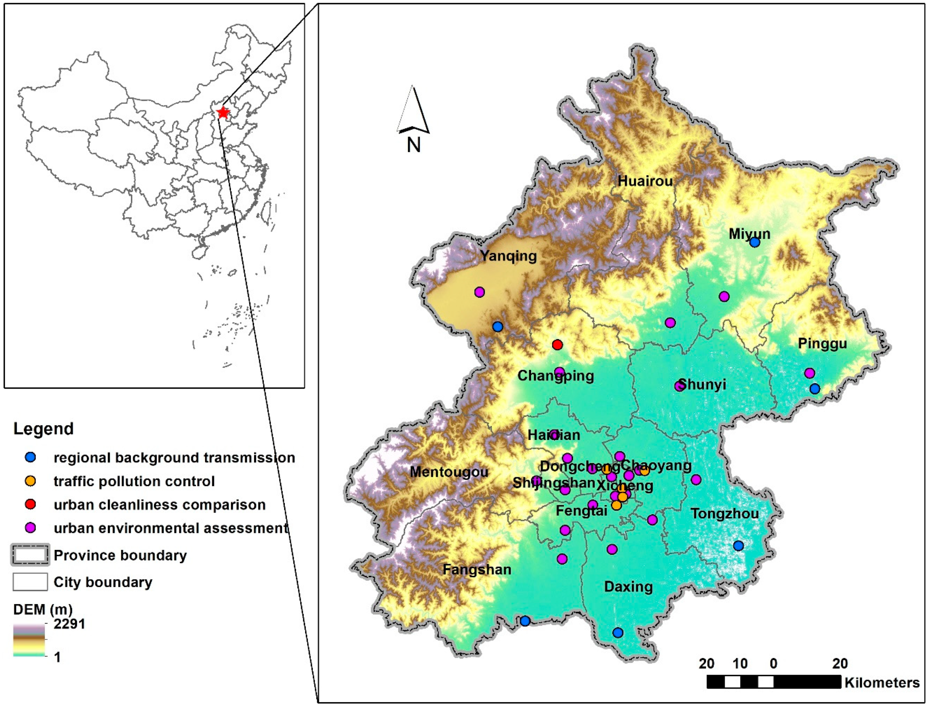
2.1. Study Area and PM2.5 Measurements

Beijing, the capital city of China, was chosen as the study area (Figure 1). It is situated in the northern portion of the North China Plain and has 16 districts. The Beijing Municipal Environmental Monitoring Center (BMEMC) is responsible for measuring and distributing PM2.5 concentrations. A total of 35 monitoring sites have been established across the domain of Beijing, with 23 sites for urban environmental assessment (UEA), six sites for regional background transmission (RBT), five sites for traffic pollution control (TPC), and one site for urban cleanliness comparison (UCC). UEA stations serve to assess the average level and variations in air quality in the urban environment. RBT stations serve to represent the regional background level of air quality and the regional transmission of atmospheric pollutants. RBT stations are distributed near the city boundaries to the northwest, northeast, east, south, and southwest. TPC stations are all located in downtown areas and monitor the influence of traffic on air quality. The sole UCC station represents the pollution level in urban areas assuming no influence of urban activities. In this study, hourly PM2.5 measurements observed at all monitoring sites in 2014 were downloaded from the BMEMC air quality releasing platform (http://zx.bjmemc.com.cn), and daily averaged PM2.5 concentrations were calculated as the dependent variable.

2.2. VIIRS IP AOD Retrievals

VIIRS is a cross-track scanning radiometer onboard the Suomi National Polar-Orbiting Partnership (Suomi-NPP) satellite with a 1:30 pm local solar time ascending node. It is expected to continue the decade-long measurement series initiated by MODIS. It contains three types of bands: imagery bands (375 m at nadir), moderate bands (M bands, 750 m at nadir), and day/night bands (750 m across scan). The VIIRS aerosol algorithms, with a heritage from MODIS aerosol algorithms, use M bands to produce the full set of aerosol parameters contained in the IP, including AOD at 550 nm [36]. VIIRS IP AOD data (contained in IVAOT files named ‘faot550’) for 2014 in Beijing were collected from the Comprehensive Large Array-data Stewardship System (CLASS) (www.class.noaa.gov). Corresponding terrain-corrected geo-location files (contained in GMTCO files named ‘Longitude’ and ‘Latitude’) for these AOD data were also downloaded from CLASS for geometric correction purposes. To minimize the potential negative effects of deviations in VIIRS IP AOD retrievals on PM2.5 estimates, only good AOD data (quality assurance flag = 0) were retained.

2.3. GEOS FP Meteorological Data

Meteorological conditions influence and hence can improve PM2.5-AOD relationships [37]. Global Earth Observing System Forward Processing (GEOS FP) gridded meteorological data for 2014 covering Beijing were collected from the Dalhousie data archive (ftp://rain.ucis.dal.ca/ctm). GEOS FP is the most recent validated GEOS system and provides meteorological fields at finer spatial (0.25° latitude × 0.3125° longitude) and temporal resolution (1-h or 3-h) over China [38,39]. Downloaded files named GEOSFP.YYYYMMDD.A1.025×03125.CH.nc, where YYYY is the year, MM is the two-digit month of the year, and DD is the two-digit day of the month, have a time interval of one hour. These files contain the planetary boundary layer height (PBLH) above the surface, temperature at 2 m above displacement height (T2M), total surface precipitation flux (PRCP), surface level pressure (PS), eastward wind at 10 m above displacement height (U10M), and northward wind at 10 m above displacement height (V10M) from 0:30 UTC to 23:30 UTC. Values of these variables at 5:30 UTC were extracted to correspond to the VIIRS overpass time. Downloaded files named GEOSFP.YYYYMMDD.A3dyn.025×03125.CH.nc have a time interval of three hours and contain 72 layers of relative humidity from 1:30 UTC to 22:30 UTC. The mean value of relative humidity in PBLH (RH_PBL) between 4:30 UTC and 7:30 UTC was extracted to correspond to the VIIRS overpass time.

2.4. Satellite-Retrieved NO2 and NDVI Data

Anthropogenic emissions and dry deposition on natural surfaces such as vegetation increase or decrease PM2.5 concentrations [40,41] and hence can adjust PM2.5-AOD relationships. This study selected NO2 from the previous day (NO2_Lag) as a proxy for anthropogenic emissions [42] and Normalized Difference Vegetation Index (NDVI) as a reflection of variations in vegetation [43]. NO2 data for 2014 covering Beijing with a resolution at 0.25° × 0.25° and 1-d based on the Ozone Monitoring Instrument were obtained from the Tropospheric Emission Monitoring Internet Service [44] (http://www.temis.nl/airpollution/no2col/no2regioomi_v2.php). NDVI data for 2014 covering Beijing with a resolution of 1-km and 16-d based on MODIS sensors came from the Level-1 and Atmospheric Archive and Distribution System (LAADS) (https://ladsweb.modaps.eosdis.nasa.gov/search/). Terra (code: MOD13A2) and Aqua (code: MYD13A2) satellite observations were combined to improve the temporal resolution to 8-d.

2.5. Data Integration

These multi-source data can be divided into point data (PM2.5 measurements) and raster data (VIIRS IP AOD retrievals, GEOS FP meteorological data, and satellite-retrieved NO2 and NDVI data). A 750 m × 750 m grid was created over Beijing, and the raster data were resampled to this grid using the bilinear interpolation method. The cell values of the resampled raster data were then extracted to the PM2.5 monitoring sites. Regression mapping and model datasets subsequently emerged.

2.6. Model Development and Validation

Based on previous two-stage models [11,17,35], a nested spatiotemporal statistical model was developed in hopes of improving the accuracy and coverage of PM2.5 estimates as well as capturing the spatiotemporal heterogeneities of PM2.5-AOD relationships. The nested spatiotemporal statistical model was composed of two parts: a nested time fixed effects regression (TFER) model and a series of GWR models with adaptive temporal scales. The first-stage nested TFER model was composed of three separate TFER models with daily, weekly, and monthly intercepts, which shared similar model structures as follows:
PM2.5,sd = λd + βAODAODsd + [βPBLHPBLHsd] + [βRH_PBLRH_PBLsd] + [βT2MT2Msd] + [βPRCPPRCPsd] + [βPSPSsd] + [βU10MU10Msd] + [βV10MV10Msd] + [βNO2_LagNO2_Lagsd] + [βNDVINDVIsd] + εsd,
PM2.5,sd = λw + βAODAODsd + [βPBLHPBLHsd] + [βRH_PBLRH_PBLsd] + [βT2MT2Msd] + [βPRCPPRCPsd] + [βPSPSsd] + [βU10MU10Msd] + [βV10MV10Msd] + [βNO2_LagNO2_Lagsd] + [βNDVINDVIsd] + εsd,
PM2.5,sd = λm + βAODAODsd + [βPBLHPBLHsd] + [βRH_PBLRH_PBLsd] + [βT2MT2Msd] + [βPRCPPRCPsd] + [βPSPSsd] + [βU10MU10Msd] + [βV10MV10Msd] + [βNO2_LagNO2_Lagsd] + [βNDVINDVIsd] + εsd,
where PM2.5,sd, AODsd, PBLHsd, RH_PBLsd, T2Msd, PRCPsd, PSsd, U10Msd, V10Msd, and NDVIsd are the PM2.5 (μg/m3), AOD (unitless), PBLH (km), RH_PBL (unitless), T2M (K), PRCP (kg/m2/s2), PS (hPa), U10M (m/s), V10M (m/s), and NDVI (unitless) at monitoring site s during day d; except for PM2.5,sd, the remaining have their corresponding coefficients βAOD, βPBLH, βRH_PBL, βT2M, βPRCP, βPS, βU10M, βV10M, and βNDVI; NO2_Lagsd is the NO2 (1015 molec/cm2) at monitoring site s during day d-1, and βNO2_Lag is the corresponding coefficient; λd, λw, and λm are the nested intercepts for each day, week, and month; [] around the variable and its coefficient indicates that the variable and its coefficient might be incorporated according to the process of determining the best model structure as described below; and εsd represents the error term at monitoring site s during day d.
To determine the best model structure for the TFER models with daily, weekly, and monthly intercepts, all possible combinations of variables were examined. At the significance level of α = 0.05, the TFER models with daily, weekly, and monthly intercepts whose slopes passed the statistical test were first retained. These models were then sorted according to the number of statistically significant intercepts and the adjusted goodness of fit (R2) in descending order. The best TFER models with daily, weekly, and monthly intercepts that had the highest adjusted goodness of fit (R2) were eventually determined from the top ten candidate models. Appendix A provides screenshots of these processes. The TFER model with daily intercepts was used to predict PM2.5 concentrations for days that had a model dataset, the model with weekly intercepts to predict PM2.5 concentrations for days that did not have a model dataset, and the model with monthly intercepts to predict PM2.5 concentrations for weeks that did not have a model dataset.
The second-stage GWR model used the residuals from the first-stage nested TFER model as the dependent variable and the VIIRS IP AOD as the independent variable. Noting that the GWR model was more suitable for analyzing spatial data, the second-stage GWR model was constructed using the average values of dependent and independent variables during a specific period. The model structure is as follows:
Residualsp = βIntercept,sp + βAOD,spAODsp + εsp,
where Residualsp and AODsp are the averaged residual from the first-stage TFER model and the AOD at monitoring site s during period p, respectively; βIntercept,sp and βAOD,sp are the location-specific intercept and slope; and εsp is the error term at monitoring site s during period p.
The value of p can be selected according to different purposes. It could be set to one day to produce daily PM2.5 estimates with higher accuracy, assuming that sufficient model datasets are available for each day. This was not true in this study, and therefore a nested TFER model was developed in the first stage. Five GWR models were calibrated for each of four seasons and for the entire year to obtain an accurate spatial distribution of PM2.5 concentrations during these periods. Because the potential maximum number of model datasets during this stage would be 35, which is a rather small number, the best fixed bandwidth for estimating coefficients was determined by minimizing the corrected Akaike Information Criterion (AICc). The bandwidth controls the size of the kernel function of the GWR model [45]. In other words, it specifies the spatial extent of the data points used to calibrate the model. AICc was computed from a measure of the divergence between observed and fitted values and a measure of model complexity [46]. The lower the AICc, the better was the model.
Sample-based ten-fold cross validation (CV) was used to assess the performance of the first-stage nested TFER model. For the TFER models with daily, weekly, and monthly intercepts, the model dataset was first randomly and equally split into ten subsets with the condition that all the days, weeks, and months of each subset must appear in the remaining subsets. This condition was incorporated so that predictions could be made for each subset using the model fitted from the other nine subsets. The rest of the process was similar: repeat using nine subsets to fit the model and use the fitted model to predict the remaining subset until all the subsets have been predicted; regress the predicted PM2.5 on the observed PM2.5 and calculate the R2, mean prediction error (MPE), and root mean square error (RMSE); and use these statistics to assess model performance.

2.7. PM2.5 Prediction

Daily PM2.5 estimates were readily obtained by combining the first-stage nested TFER model and the regression mapping dataset. Note that these daily PM2.5 estimates had different accuracies because different TFER models with daily, weekly, or monthly intercepts were used on certain days depending on the availability of a model dataset. Therefore, different weights should be assigned to different daily estimates when using them to derive seasonal and annual PM2.5 estimates. In this study, the sample-based ten-fold CV R2 values of the TFER models with daily, weekly, and monthly intercepts were used as the weight for the daily PM2.5 estimates calculated from those models. The weighted seasonal and annual PM2.5 estimates were further corrected by the second-stage GWR models.

3. Results

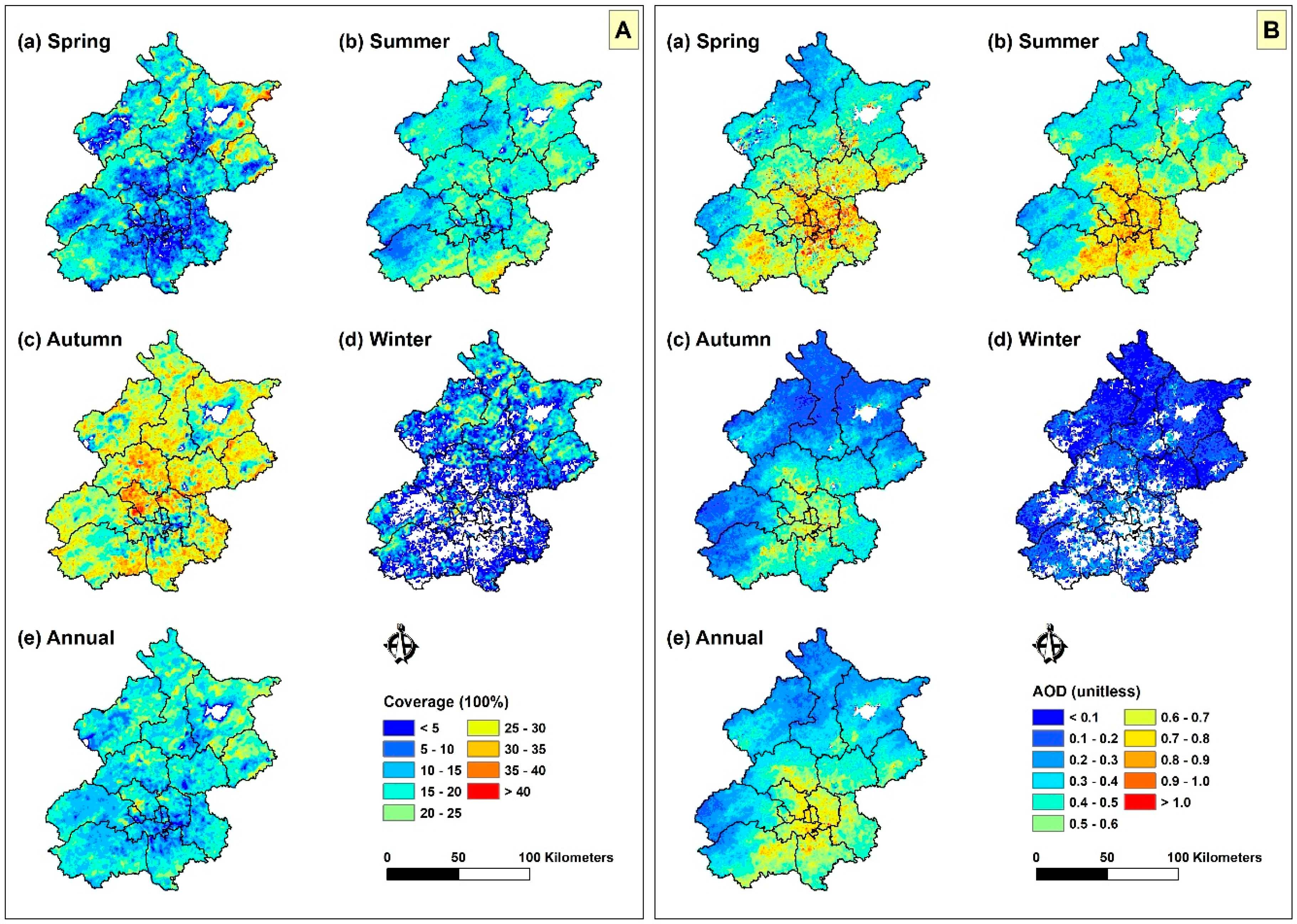
3.1. Spatiotemporal Coverage and Distribution of VIIRS IP AOD

Figure 2 illustrates the seasonal-spatial distribution of the VIIRS IP AOD coverage and average. Spatially, low spatiotemporal coverage and high VIIRS IP AOD values occurred in urban centers, whereas high spatiotemporal coverage and low VIIRS IP AOD values mainly appeared on the urban periphery. Temporally, autumn had much higher spatiotemporal coverage of VIIRS IP AOD than the other seasons, but its average AOD values were lower than those in spring and summer. Overall, the VIIRS IP AOD had an average spatiotemporal coverage and value of 16.12% and 0.4039, respectively, across Beijing in 2014. The missing data problem of the VIIRS IP AOD is somewhat severe, indicating the necessity of developing a nested spatiotemporal statistical model.

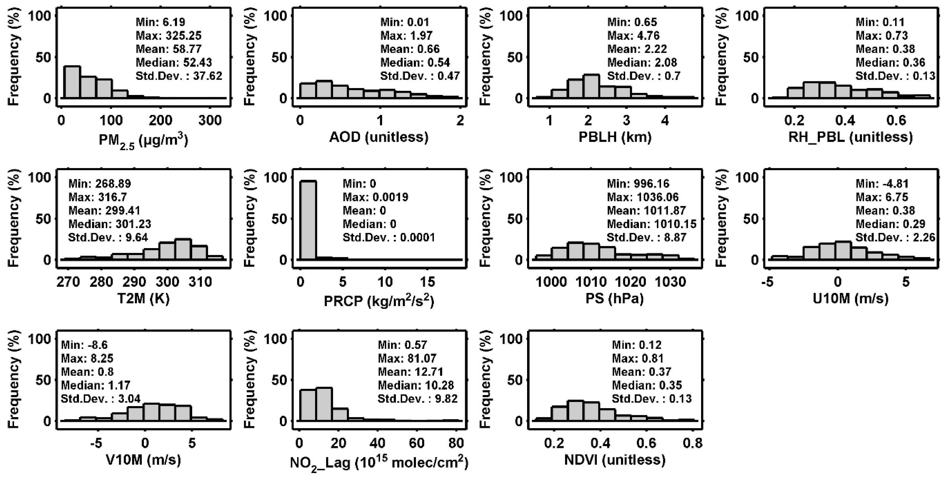
3.2. Descriptive Analysis of Model Dataset

Figure 3 illustrates the histogram and several common statistics of all variables in the model dataset. Except for PRCP, the remaining variables were approximately normally distributed (AOD, PBLH, RH_PBL, T2M, PS, U10M, V10M, and NDVI) or log-normally distributed (PM2.5 and NO2_Lag). Overall, the mean values of PM2.5 and AOD were 58.15 μg/m3 and 0.65, respectively, indicating that the loadings of both surface and total aerosol particles were high in Beijing.

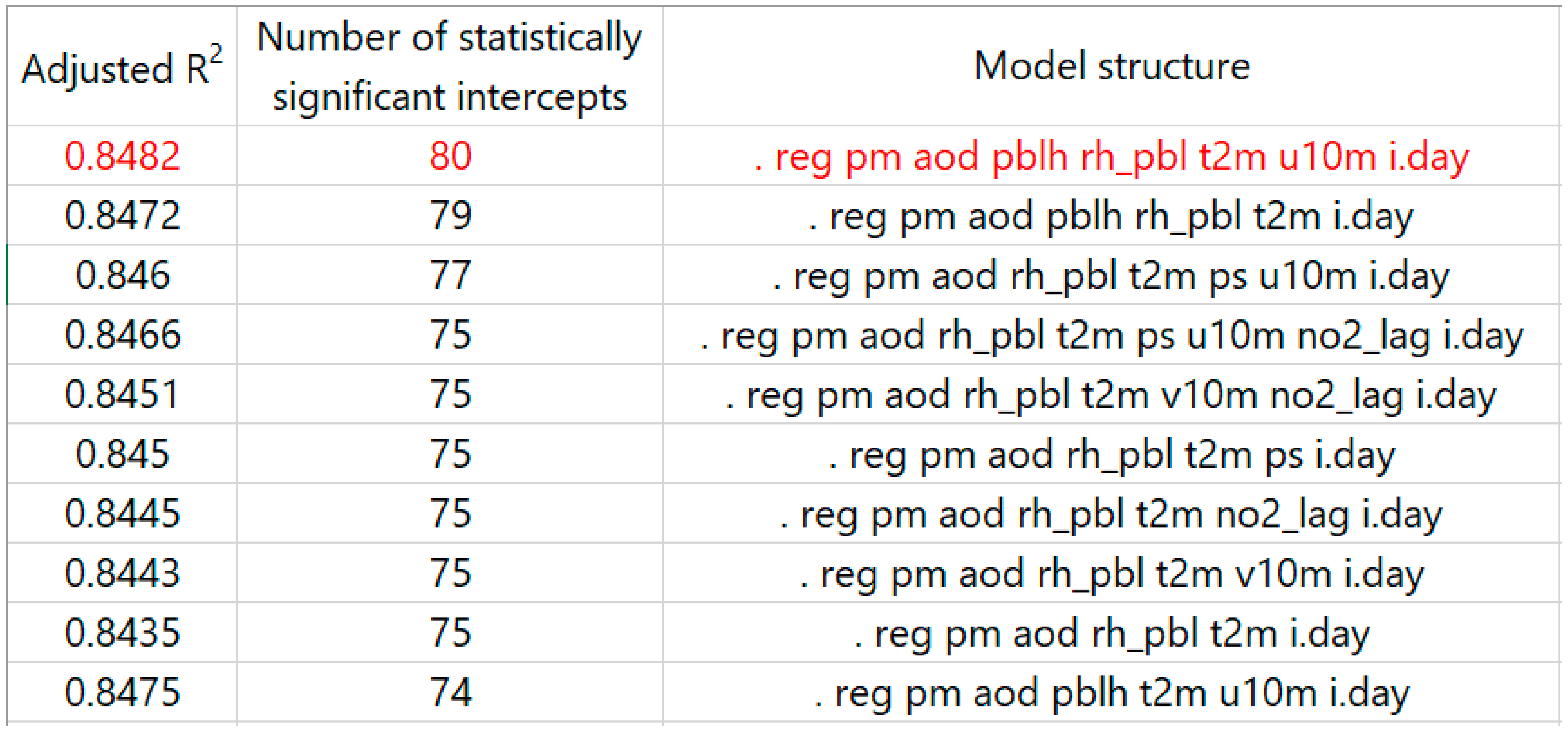
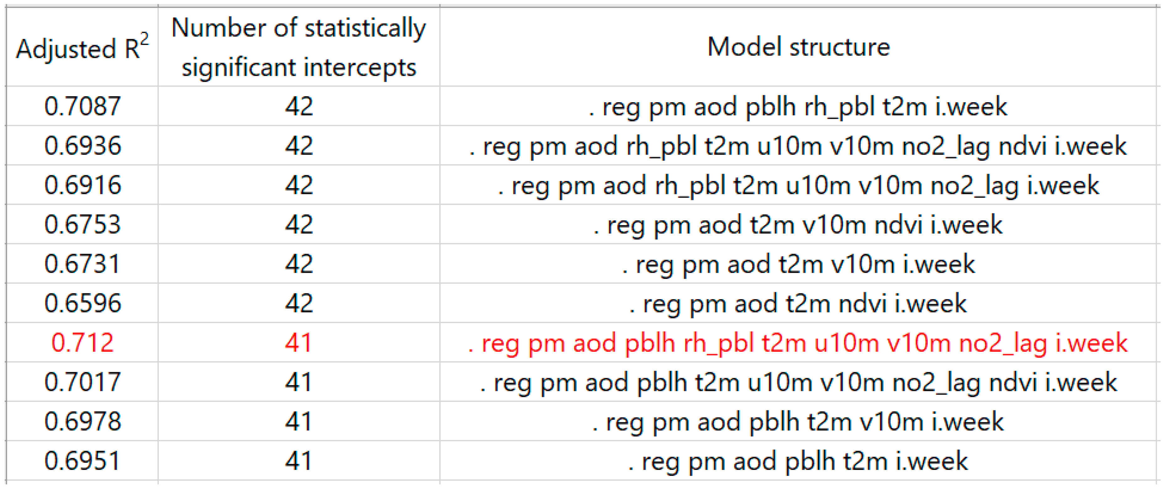
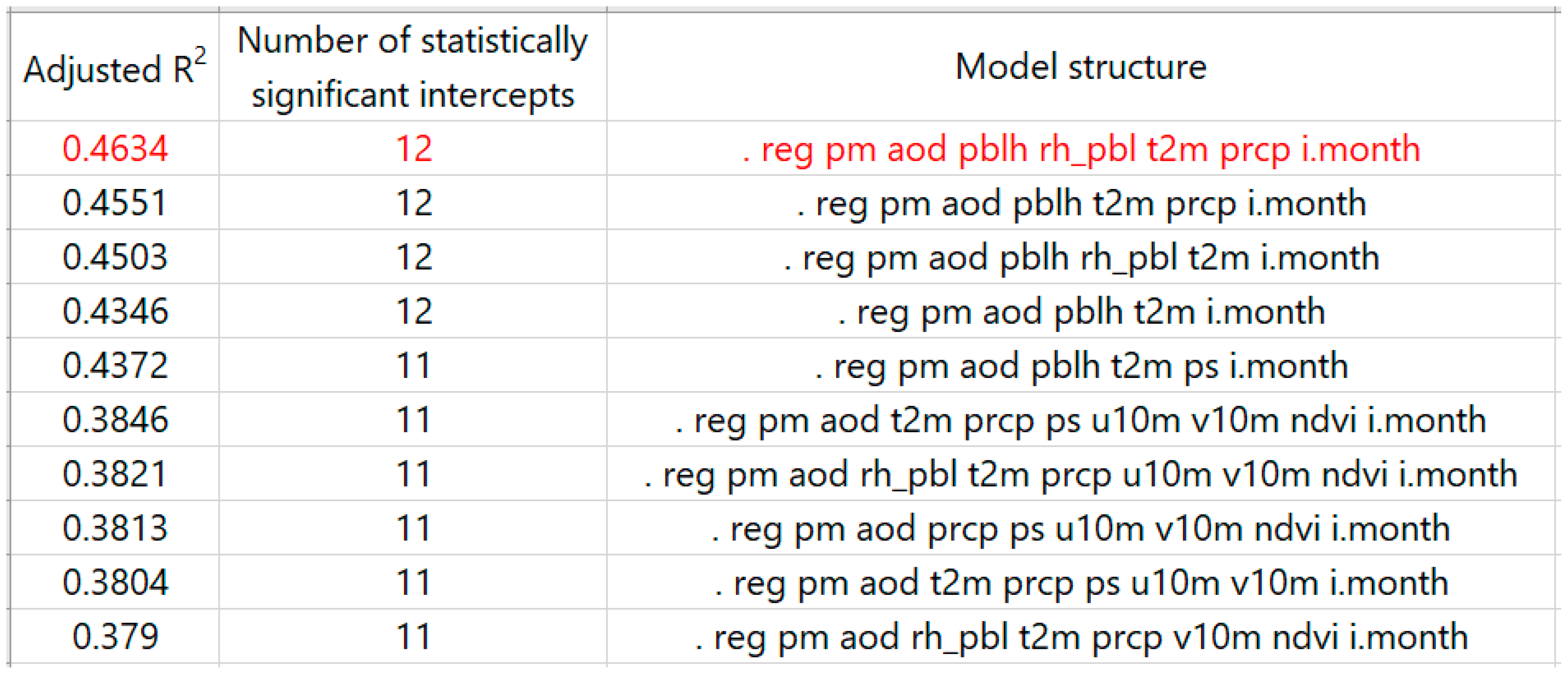
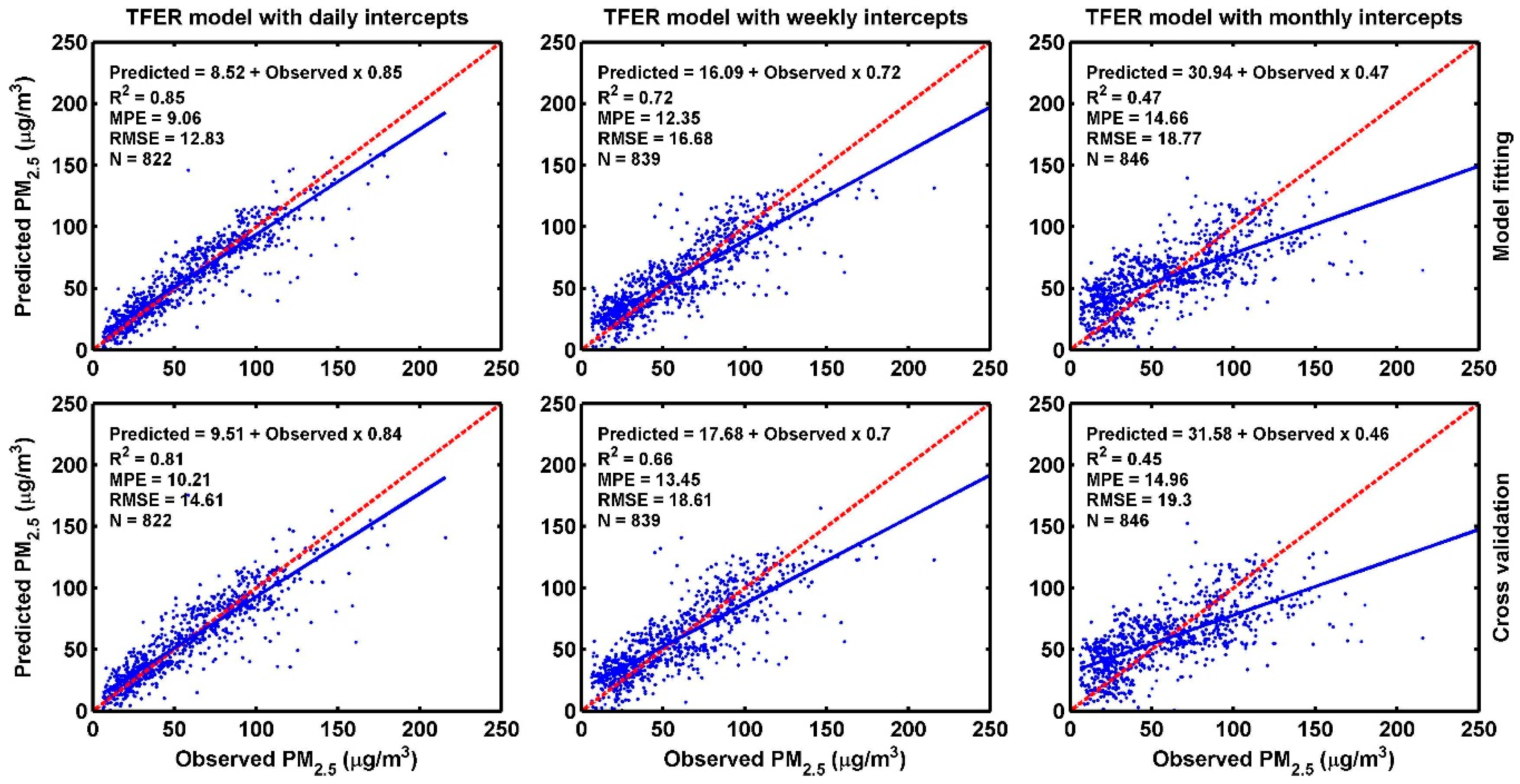
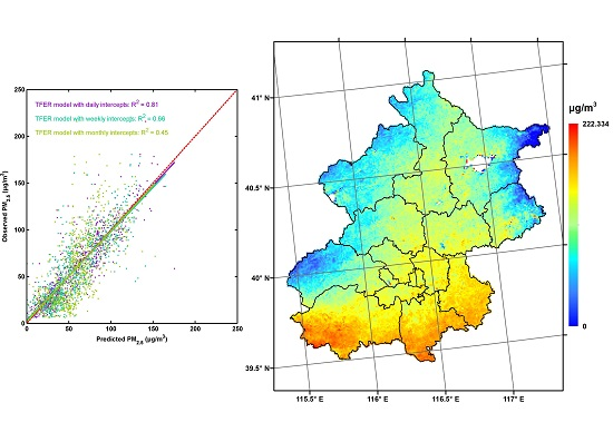
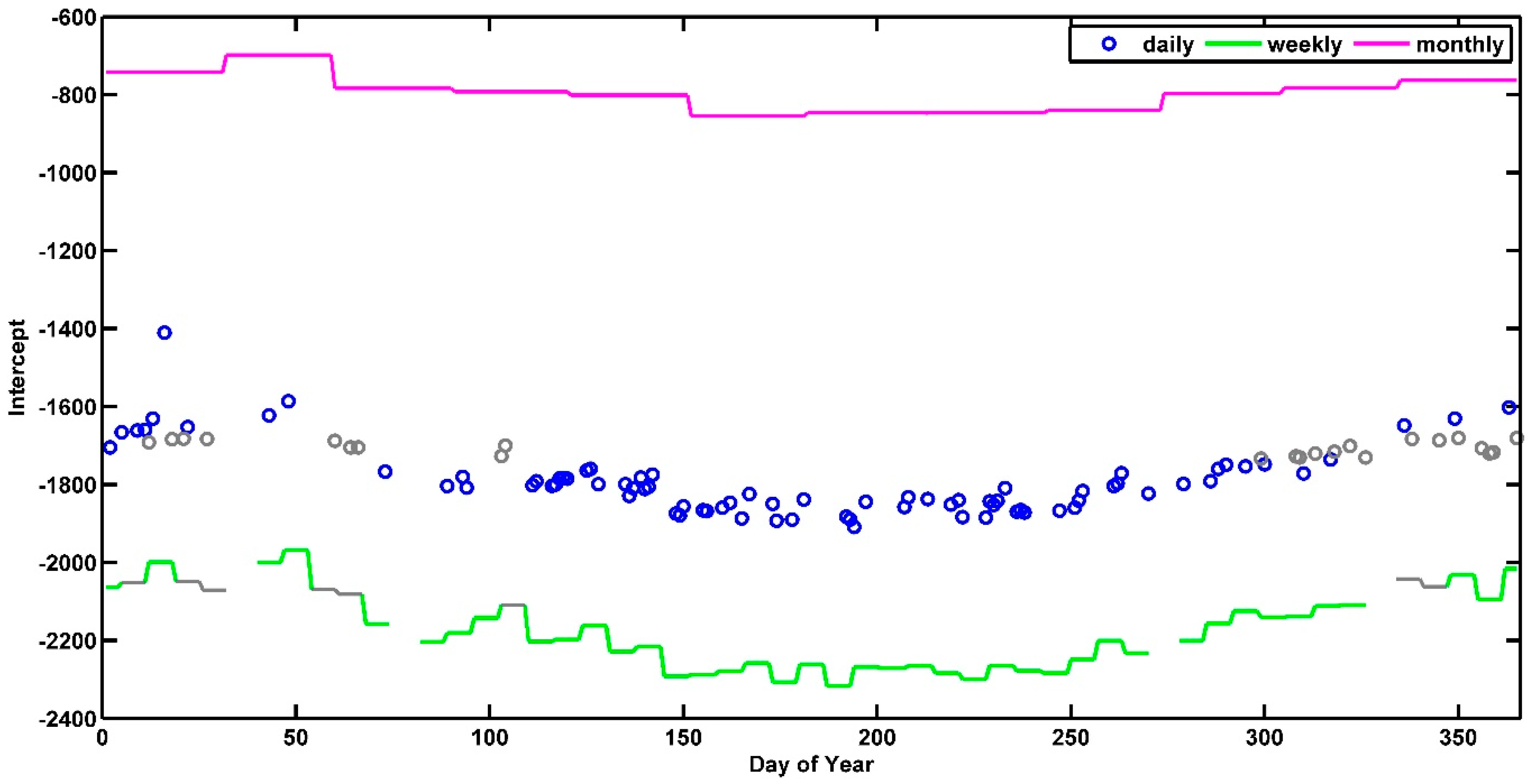
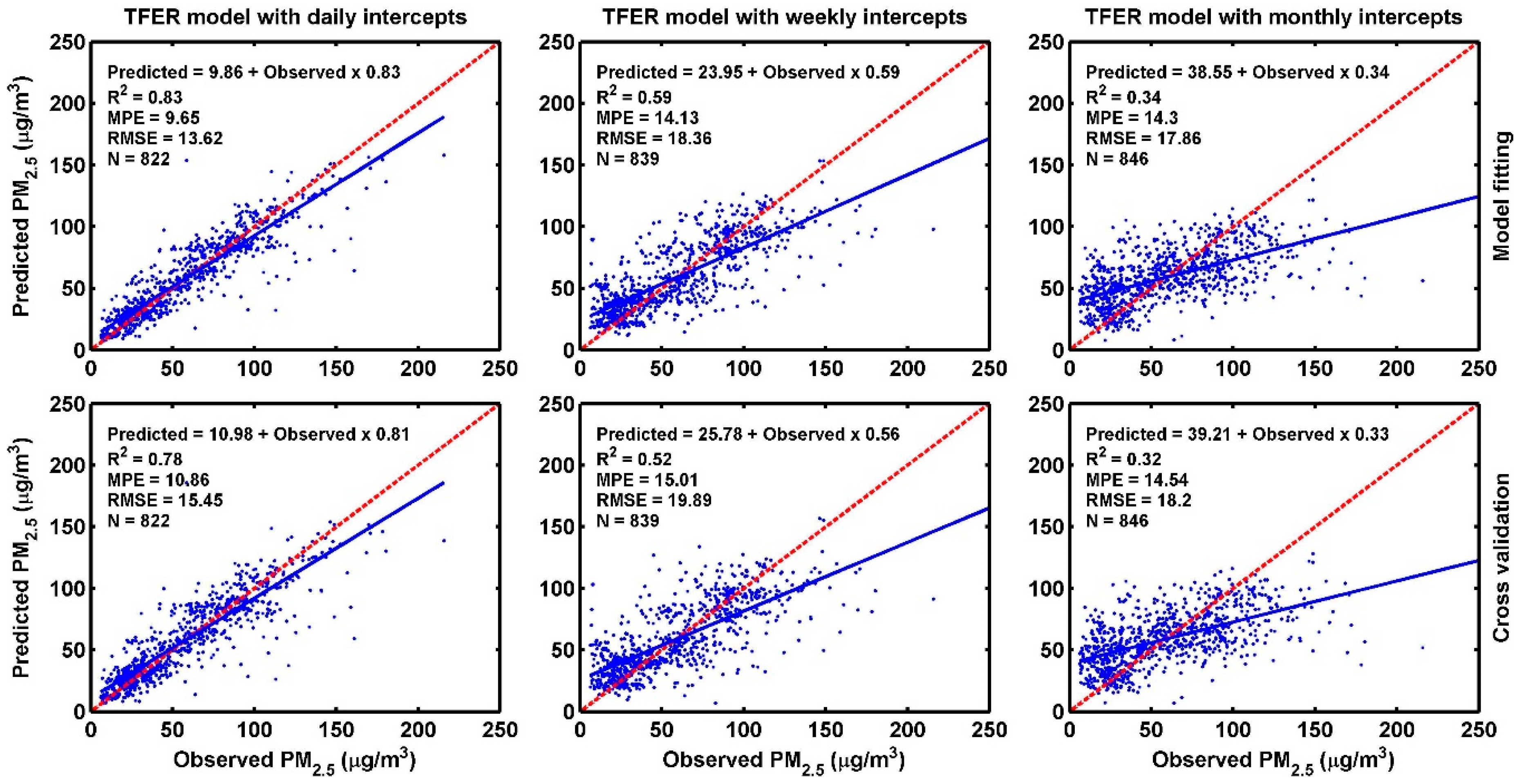
3.3. Results of Model Fitting and Validation

Table 1 shows the coefficients of the independent variables of the first-stage TFER models with daily, weekly, and monthly intercepts. PS and NDVI did not appear in any TFER models and were therefore omitted from Table 1. Except for PRCP, the coefficients of the remaining variables had reasonable values. Although PRCP had an extremely large positive coefficient, the maximum value of the PRCP observations was only 0.00019, meaning that the products of the coefficient and the observations would not be very large and that the final PM2.5 estimates would not be significantly biased. Figure 4 shows the variations of daily, weekly, and monthly intercepts. Clearly, the intercepts in winter and spring were always larger than those in summer and autumn. Because the remaining coefficients in each TFER model were fixed, such variations, to some extent, indicated that PM2.5 concentrations during winter and spring were probably larger than those during summer and autumn under the same condition. The proportion of statistically significant intercepts approached 77.67%, 83.67%, and 100% for the TFER models with daily, weekly, and monthly intercepts, respectively, showing the goodness of model fitting.
Figure 5 illustrates the model fitting and sample-based ten-fold CV results for the first-stage nested TFER model. Considering the behavior of the R2 and MPE (RMSE) of the model during ten-fold CV, from the TFER model with monthly intercepts to the TFER model with weekly intercepts and from this version of the model to the TFER model with daily intercepts, R2 increased by 46.67% and 22.73%, respectively, and MPE (RMSE) decreased by 27.08% (22.11%) and 29.40% (27.47%), respectively. This indicates that the PM2.5-AOD relationship presents strong temporal heterogeneities. Varying intercepts with a shorter time interval could capture more temporal heterogeneities and hence might be more appreciated. Model overfitting problems existed to different extents in the first-stage nested TFER model. For days with a model dataset in which the TFER model with daily intercepts was used, the R2 decreased by 4.71% from model fitting to ten-fold CV. The corresponding values were 8.33% and 4.26%, respectively, in the TFER model with weekly and monthly intercepts. These relatively small values indicate that the model overfitting problem was not very severe. The proportion of daily PM2.5 estimates explained ranged from 0.45 to 0.81 according to the ten-fold CV results. Although 0.45 was not a high value, it yielded more information than if no PM2.5 estimates were retrieved. In addition, the correlation coefficient between predicted and observed PM2.5 could approach 0.67, which is not a bad result.
By removing the auxiliary variables, an AOD-only nested TFER model was fitted. Figure 6 illustrates its model fitting and sample-based ten-fold CV validation results. It is apparent that all the R2 declined, whereas all the MPE and RMSE increased. Further calculations revealed that when moving from the AOD-only model to the full model, R2 increased by 3.85%, 26.92%, and 40.63% for the TFER models with daily, weekly, and monthly intercepts, respectively, during sample-based ten-fold CV. These values indicated the relative role of varying intercepts and auxiliary variables on adjusting PM2.5-AOD relationships. When varying intercepts with shorter time intervals were incorporated, the role of auxiliary variables became less important. In this study, the auxiliary variables especially the meteorological data, did not have high spatial resolutions, but they were nevertheless used by interpolating them to the same spatial resolution as the VIIRS IP AOD. This may have introduced some uncertainties, but fortunately the degree to which uncertainties occurred was not large because the values of the sample-based ten-fold CV R2 of the AOD-only models shown in Figure 6 were relatively high. It is feasible to use only AOD itself to derive PM2.5 concentrations using a spatiotemporal statistical model (e.g., [16]) when high-coverage satellite-retrieved AOD are available, but high-resolution auxiliary variables are very difficult to access.
By removing the VIIRS IP AOD variable, a non-AOD nested TFER model was fitted. Table 2 lists the results of F tests between the full and non-AOD models. It shows that the incorporation of the VIIRS IP AOD retrievals significantly improved the performance of the TFER models with daily, weekly, and monthly intercepts at α = 0.05. In addition, the extent to which the improvement occurred follows an increasing order of the TFER models with daily, weekly, monthly intercepts according to the size of the F values.
Table 3 lists the estimated best bandwidth, minimum AICc, range of the intercepts, AOD coefficients, and local R2 for each GWR model. Except for the bandwidth in spring and winter, which was almost double those in the other seasons and the entire year, all the other parameters had reasonable values and ranges. Spatially varying coefficients of the intercept and AOD indicated that the second-stage GWR captured the spatial heterogeneities of the PM2.5-AOD relationships. Spatially varying local R2 showed the extent to which this improvement was achieved, up to a maximum of 0.672. Therefore, the performance of the first-stage nested TFER model was improved.

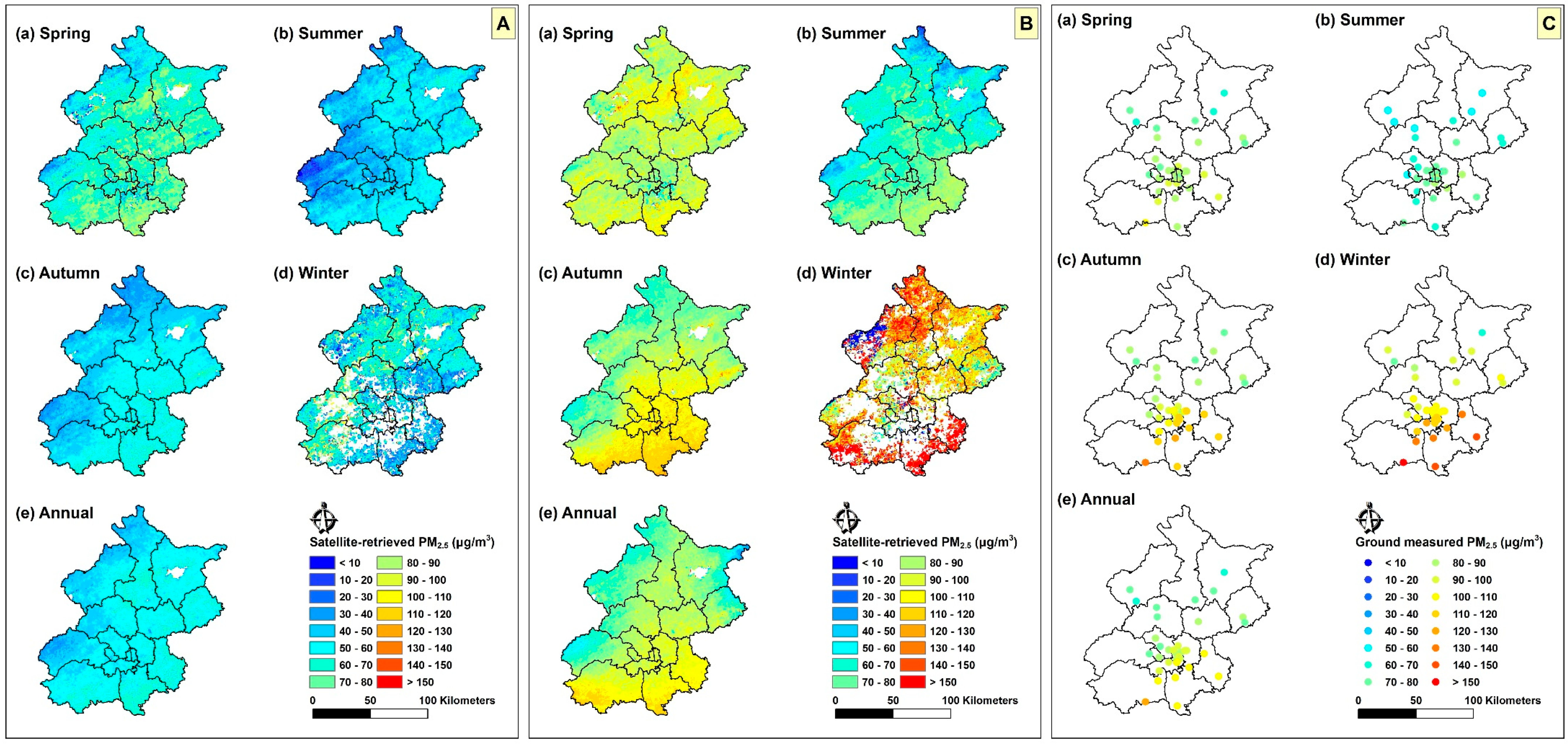
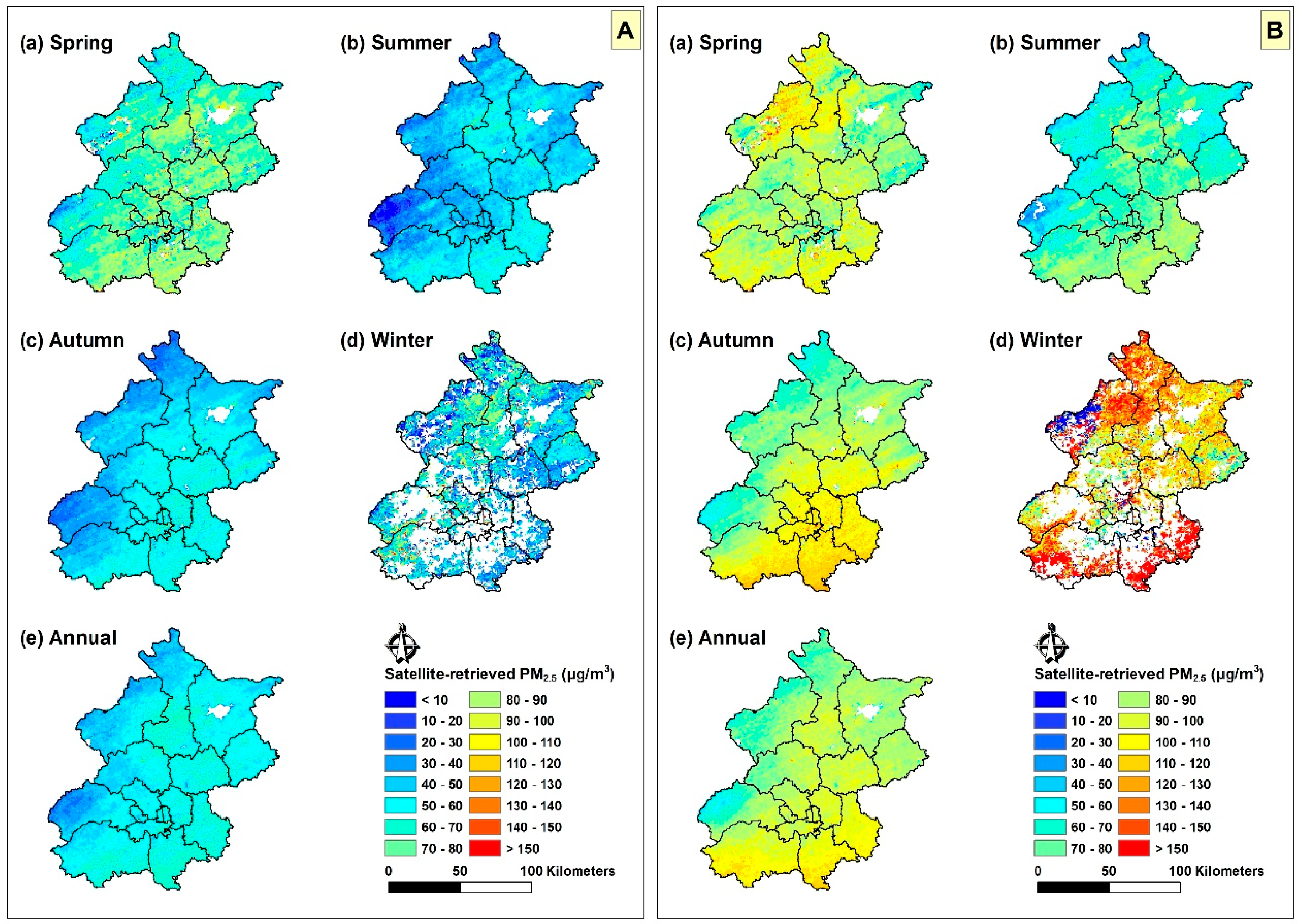
3.4. Results of PM2.5 Prediction

Figure 7 illustrates the seasonal-spatial distribution of satellite-based and ground measured PM2.5 concentrations. The PM2.5 predictions from the overall model were higher than those from the first-stage nested TFER model. These higher values were much closer to the real level shown in Figure 7C, indicating the necessity and effectiveness of adding the second-stage GWR models. In terms of the spatiotemporal pattern of PM2.5 pollution in Beijing, during summer, autumn, and the entire year, from the northwestern areas to the southeastern areas, a gradient of slight to severe PM2.5 pollution was observed. These gradual changes were consistent with previous studies [16,47] but this study provides more spatial detail thanks to the high spatial resolution of the VIIRS IP AOD retrievals. However, similar gradual changes did not occur during spring and winter, but noisy distributions were found instead. This phenomenon may be attributed to very low spatiotemporal coverage (Figure 2) plus the insufficiently high accuracy [22,23,24] of the VIIRS IP AOD retrievals, which constitutes one of the deficiencies of these retrievals and deserves attention and improvement in the future. In addition, the fact that large quantities of coarse particles intrude into Beijing during spring [48] might also badly influence the accuracy of PM2.5 estimates during this season. Seasonally, it was only possible to conclude roughly that PM2.5 pollution during summer was relatively slight.

4. Discussion

To demonstrate the potential benefits and deficiencies of the nested spatiotemporal statistical model (hereafter referred to as the nested model), a non-nested spatiotemporal statistical model (hereafter referred to as the non-nested model) was developed and used to predict PM2.5 concentrations. The difference between the nested and non-nested models was that the latter used the TFER model with daily intercepts only at the first stage. Consequently, daily intercepts and hence PM2.5 concentrations could not be obtained for days without a model dataset. Figure 8 shows the PM2.5 prediction maps from the non-nested model; they resemble those from the nested model, as shown in Figure 7. Nevertheless, one obvious difference was observed in winter (N.B. Also the remaining seasons and the entire year, shown in Figure 9B), during which the nested model produced more PM2.5 estimates than the non-nested model. The absence of a model dataset on a certain day only meant that data integration at the PM2.5 ground monitors failed, but the VIIRS IP AOD and other auxiliary variables may still have existed at other locations on that day. The nested model used weekly and monthly intercepts to predict PM2.5 concentrations on those days, thus maximizing the use of existing datasets and leading to a better coverage of the final PM2.5 estimates.
The predicted PM2.5 concentrations from the nested and non-nested models were further compared with the observed PM2.5 concentrations from the 35 monitoring sites. Figure 9B shows that the numbers of available daily PM2.5 estimates to calculate seasonal and annual PM2.5 estimates all increased, with an increase of approximately 50% in summer, autumn, and the entire year. Figure 9A shows that the accuracy of seasonal and annual PM2.5 estimates increased or declined during different seasons and the entire year. Generally, the accuracy of seasonal and annual PM2.5 estimates based on daily PM2.5 estimates is subject to two factors: accuracy and the number of daily PM2.5 estimates. More available daily PM2.5 estimates with higher accuracy produce more accurate seasonal and annual PM2.5 estimates. The situation was, however, slightly more complex in this study because the nested model provided more available daily PM2.5 estimates with lower accuracies. Therefore, the eventual accuracy of the seasonal and annual PM2.5 estimates was dependent on the tradeoff between these two opposing factors. The nested model increased the number of daily PM2.5 estimates to a very limited degree in winter and spring given that the original spatiotemporal coverages of the VIIRS IP AOD retrievals during these two seasons were rather low, the advantages of which did not outweigh the disadvantages of the accumulation of lower accuracies, thereby leading to a decline, or more strictly speaking, a fluctuation, in the accuracies of winter and spring PM2.5 estimates. The nested model significantly increased the number of daily PM2.5 estimates in summer, autumn, and the entire year, the advantages of which outweighed the disadvantages of the accumulation of lower accuracies, thereby resulting in improved accuracies of summer, autumn, and annual PM2.5 estimates.
The present work, to some extent, resembles the work by Ma et al. [15], who developed a nested linear mixed effects (LME) regression model to improve the accuracy of PM2.5 estimates on days without a model dataset. As stated in previous work by the authors [17], the LME model is more widely used for analyzing hierarchical data and accommodating complicated hierarchical correlations of observations, whereas the TFER model, which is derived from panel data regression models, is relatively easier to calibrate and to use for prediction. Because the sample size, variables, and study area differed between the work by Ma et al. [15] and the present work differed, it was difficult to compare directly the sample-based ten-fold CV R2 values of these two studies. Nevertheless, it could be roughly concluded that a comparable model performance has been obtained without specifying varying slopes, which may increase the model’s complexity, indicating the feasibility of the combination of VIIRS IP AOD retrievals and the nested TFER model in Beijing city. In addition, the modeling steps can be easily repeated in other cities, meaning that the present work contributes not only a specific model for Beijing city, but also a modeling framework for similar cities, as long as high spatial resolution satellite-retrieved AOD and correlated auxiliary variables are accessible. Attention should be paid to selecting appropriate variables because factors influencing PM2.5-AOD relationships vary from one geographical area to another.
One limitation associated with this study is that no measures were taken to supplement the missing data in the VIIRS IP AOD retrievals. A nested model was developed to make the maximum use of these retrievals, but it was still difficult to produce daily PM2.5 estimates with high accuracy for each day. Therefore, the choice was made to calibrate and validate the five GWR models at seasonal and annual scales in this study. One possible explanation of the low spatiotemporal coverage of the VIIRS IP AOD retrievals was that the current version of the VIIRS over-land algorithm, mostly based on the MODIS atmospheric correction algorithm [49], does not retrieve aerosol properties over bright surfaces, in cloud-affected pixels, over inland water such as the Great Lakes, or at night [36]. As such, a relatively low overall 16.12% spatiotemporal coverage occurred due to the limited number of clear sky days in Beijing in 2014. The value became even smaller during winter when leaves falling leading to more bright pixels. Developing specific algorithms for bright areas to retrieve AOD from the VIIRS will probably benefit mitigating this missing data problem. The LAADS Distributed Active Archive Center (DAAC), for instance, has recently released the Suomi-NPP VIIRS Deep Blue Aerosol products (https://ladsweb.modaps.eosdis.nasa.gov/alerts-and-issues/?id=25803). Integrating AOD retrievals from other sources such as 1-km MAIAC AOD could also be very helpful, thereby generating seasonal and annual PM2.5 estimates as well as more days of PM2.5 estimates with higher accuracy and coverage. Another limitation of this study is that a large number of independent variables proposed in previous studies were not tested here (e.g., the accuracy of the PM2.5 estimates during spring could be potentially improved if variables representing coarse vs. fine fraction of aerosols were incorporated). The authors firmly believe that the model structure for the first-stage nested TFER model will prove to be more suitable and robust with more variables tested in the future.

5. Conclusions

According to the authors’ knowledge, this study is one of the earliest applications of the most recent high-resolution VIIRS IP AOD to predict PM2.5 concentrations across Beijing at a 750-m spatial resolution. The results were, on the whole, satisfactory despite some limitations. It could be concluded that the combination of the VIIRS IP AOD and the nested spatiotemporal statistical model could estimate urban PM2.5 concentrations. The daily PM2.5 estimates explained ranged from 0.45 to 0.81. More daily PM2.5 estimates were derived, and the accuracies of the summer, autumn, and annual PM2.5 estimates were improved based on the nested spatiotemporal statistical model. This study can surely benefit fine-scale PM2.5-related studies, such as urban-scale PM2.5 exposure assessment.

Author Contributions

Conceptualization, F.Y.; Funding acquisition, J.W. and J.P.; Investigation, F.Y. and W.L.; Methodology, F.Y.; Supervision, J.W.; Validation, F.Y.; Visualization, F.Y.

Funding

This study was financially supported by the Shenzhen Science and Technology Innovation Committee (No. JCYJ20170412150910443), National Natural Science Foundation of China (No. 41471370), The University of Hong Kong Seed Fund for Basic Research (201711159270), and China Scholarship Council (CSC).

Acknowledgments

We thank Zhongjing Jiang (PhD student from the School of Physics, Peking University) for providing information on various sources of gridded meteorological dataset. We appreciate constructive suggestions from both anonymous reviewers and academic editors.

Conflicts of Interest

The authors declare no conflict of interest. The funders had no role in the design of the study; in the collection, analyses, or interpretation of data; in the writing of the manuscript, or in the decision to publish the results.

Appendix A

Figure A1. Screenshot of determining the best model structure for the TFER model with daily intercepts.
Remotesensing 11 00841 g0a1
Figure A2. Screenshot of determining the best model structure for the TFER model with weekly intercepts.
Remotesensing 11 00841 g0a2
Figure A3. Screenshot of determining the best model structure for the TFER model with monthly intercepts.
Remotesensing 11 00841 g0a3

References

  1. Liang, C.-S.; Duan, F.-K.; He, K.-B.; Ma, Y.-L. Review on recent progress in observations, source identifications and countermeasures of PM2.5. Environ. Int. 2016, 86, 150–170. [Google Scholar] [CrossRef] [PubMed]
  2. Lelieveld, J.; Evans, J.S.; Fnais, M.; Giannadaki, D.; Pozzer, A. The contribution of outdoor air pollution sources to premature mortality on a global scale. Nature 2015, 525, 367. [Google Scholar] [CrossRef] [PubMed]
  3. Lim, S.S.; Vos, T.; Flaxman, A.D.; Danaei, G.; Shibuya, K.; Adair-Rohani, H.; AlMazroa, M.A.; Amann, M.; Anderson, H.R.; Andrews, K.G.; et al. A comparative risk assessment of burden of disease and injury attributable to 67 risk factors and risk factor clusters in 21 regions, 1990–2010: A systematic analysis for the Global Burden of Disease Study 2010. Lancet 2012, 380, 2224–2260. [Google Scholar] [CrossRef]
  4. Zhang, Q.; Jiang, X.; Tong, D.; Davis, S.J.; Zhao, H.; Geng, G.; Feng, T.; Zheng, B.; Lu, Z.; Streets, D.G.; et al. Transboundary health impacts of transported global air pollution and international trade. Nature 2017, 543, 705. [Google Scholar] [CrossRef]
  5. Seinfeld, J.H.; Pandis, S.N. Atmospheric Chemistry and Physics: From Air Pollution to Climate Change; John Wiley & Sons: New York, NY, USA, 2016. [Google Scholar]
  6. Chan, C.K.; Yao, X. Air pollution in mega cities in China. Atmos. Environ. 2008, 42, 1–42. [Google Scholar] [CrossRef]
  7. Solazzo, E.; Bianconi, R.; Pirovano, G.; Matthias, V.; Vautard, R.; Moran, M.D.; Appel, K.W.; Bessagnet, B.; Brandt, J.; Christensen, J.H. Operational model evaluation for particulate matter in Europe and North America in the context of AQMEII. Atmos. Environ. 2012, 53, 75–92. [Google Scholar] [CrossRef] [Green Version]
  8. Amanollahi, J.; Tzanis, C.; Abdullah, A.; Ramli, M.; Pirasteh, S. Development of the models to estimate particulate matter from thermal infrared band of Landsat Enhanced Thematic Mapper. Int. J. Environ. Sci. Technol. 2013, 10, 1245–1254. [Google Scholar] [CrossRef] [Green Version]
  9. Hu, X.; Waller, L.A.; Lyapustin, A.; Wang, Y.; Liu, Y. 10-year spatial and temporal trends of PM2.5 concentrations in the southeastern US estimated using high-resolution satellite data. Atmos. Chem. Phys. 2014, 14, 6301–6314. [Google Scholar] [CrossRef]
  10. Liu, Y.; Paciorek, C.J.; Koutrakis, P. Estimating regional spatial and temporal variability of PM2.5 concentrations using satellite data, meteorology, and land use information. Environ. Health Perspect. 2009, 117, 886–892. [Google Scholar] [CrossRef]
  11. Ma, Z.; Hu, X.; Sayer, A.M.; Levy, R.; Zhang, Q.; Xue, Y.; Tong, S.; Bi, J.; Huang, L.; Liu, Y. Satellite-based spatiotemporal trends in PM2.5 concentrations: China, 2004–2013. Environ. Health Perspect. 2016, 124, 184–192. [Google Scholar] [CrossRef]
  12. Liu, M.; Huang, Y.; Ma, Z.; Jin, Z.; Liu, X.; Wang, H.; Liu, Y.; Wang, J.; Jantunen, M.; Bi, J.; et al. Spatial and temporal trends in the mortality burden of air pollution in China: 2004–2012. Environ. Int. 2017, 98, 75–81. [Google Scholar] [CrossRef]
  13. Wu, J.; Zhu, J.; Li, W.; Xu, D.; Liu, J. Estimation of the PM2.5 health effects in China during 2000–2011. Environ. Sci. Pollut. Res. Int. 2017, 24, 1–13. [Google Scholar] [CrossRef]
  14. He, Q.; Huang, B. Satellite-based high-resolution PM2.5 estimation over the Beijing-Tianjin-Hebei region of China using an improved geographically and temporally weighted regression model. Environ. Pollut. 2018. [Google Scholar] [CrossRef]
  15. Ma, Z.W.; Liu, Y.; Zhao, Q.Y.; Liu, M.M.; Zhou, Y.C.; Bi, J. Satellite-derived high resolution PM2.5 concentrations in Yangtze River Delta Region of China using improved linear mixed effects model. Atmos. Environ. 2016, 133, 156–164. [Google Scholar] [CrossRef]
  16. Xie, Y.; Wang, Y.; Zhang, K.; Dong, W.; Lv, B.; Bai, Y. Daily Estimation of Ground-Level PM2.5 Concentrations over Beijing Using 3 km Resolution MODIS AOD. Environ. Sci. Technol. 2015, 49, 12280. [Google Scholar] [CrossRef]
  17. Wu, J.; Yao, F.; Li, W.; Si, M. VIIRS-based remote sensing estimation of ground-level PM2.5 concentrations in Beijing–Tianjin–Hebei: A spatiotemporal statistical model. Remote Sens. Environ. 2016, 184, 316–328. [Google Scholar] [CrossRef]
  18. Yao, F.; Si, M.; Li, W.; Wu, J. A multidimensional comparison between MODIS and VIIRS AOD in estimating ground-level PM2.5 concentrations over a heavily polluted region in China. Sci. Total Environ. 2018, 618, 819–828. [Google Scholar] [CrossRef]
  19. Liang, F.C.; Xiao, Q.Y.; Wang, Y.J.; Lyapustin, A.; Li, G.X.; Gu, D.F.; Pan, X.C.; Liu, Y. MAIAC-based long-term spatiotemporal trends of PM2.5 in Beijing, China. Sci. Total Environ. 2018, 616, 1589–1598. [Google Scholar] [CrossRef]
  20. Xiao, Q.Y.; Wang, Y.J.; Chang, H.H.; Meng, X.; Geng, G.N.; Lyapustin, A.; Liu, Y. Full-coverage high-resolution daily PM2.5 estimation using MAIAC AOD in the Yangtze River Delta of China. Remote Sens. Environ. 2017, 199, 437–446. [Google Scholar] [CrossRef]
  21. Zhang, T.; Zhu, Z.; Gong, W.; Zhu, Z.; Sun, K.; Wang, L.; Huang, Y.; Mao, F.; Shen, H.; Li, Z.; et al. Estimation of ultrahigh resolution PM2.5 concentrations in urban areas using 160 m Gaofen-1 AOD retrievals. Remote Sens. Environ. 2018, 216, 91–104. [Google Scholar] [CrossRef]
  22. Wang, W.; Mao, F.; Pan, Z.; Du, L.; Gong, W. Validation of VIIRS AOD through a Comparison with a Sun Photometer and MODIS AODs over Wuhan. Remote Sens. 2017, 9, 403. [Google Scholar] [CrossRef]
  23. Xiao, Q.; Zhang, H.; Choi, M.; Li, S.; Kondragunta, S.; Kim, J.; Holben, B.; Levy, R.; Liu, Y. Evaluation of VIIRS, GOCI, and MODIS Collection 6 AOD retrievals against ground sunphotometer observations over East Asia. Atmos. Chem. Phys. 2016, 16, 1255–1269. [Google Scholar] [CrossRef] [Green Version]
  24. Meng, F.; Cao, C.; Shao, X. Spatio-temporal variability of Suomi-NPP VIIRS-derived aerosol optical thickness over China in 2013. Remote Sens. Environ. 2015, 163, 61–69. [Google Scholar] [CrossRef]
  25. Van Donkelaar, A.; Martin, R.V.; Brauer, M.; Hsu, N.C.; Kahn, R.A.; Levy, R.C.; Lyapustin, A.; Sayer, A.M.; Winker, D.M. Global estimates of fine particulate matter using a combined geophysical-statistical method with information from satellites, models, and monitors. Environ. Sci. Technol. 2016, 50, 3762–3772. [Google Scholar] [CrossRef]
  26. Van Donkelaar, A.; Martin, R.V.; Brauer, M.; Kahn, R.; Levy, R.; Verduzco, C.; Villeneuve, P.J. Global estimates of ambient fine particulate matter concentrations from satellite-based aerosol optical depth: Development and application. Environ. Health Perspect. 2010, 118, 847–855. [Google Scholar] [CrossRef]
  27. Chen, G.; Li, S.; Knibbs, L.D.; Hamm, N.A.S.; Cao, W.; Li, T.; Guo, J.; Ren, H.; Abramson, M.J.; Guo, Y. A machine learning method to estimate PM2.5 concentrations across China with remote sensing, meteorological and land use information. Sci. Total Environ. 2018, 636, 52–60. [Google Scholar] [CrossRef]
  28. Hu, X.; Belle, J.H.; Meng, X.; Wildani, A.; Waller, L.; Strickland, M.; Liu, Y. Estimating PM2.5 Concentrations in the Conterminous United States Using the Random Forest Approach. Environ. Sci. Technol. 2017, 51, 6936. [Google Scholar] [CrossRef]
  29. Xu, Y.; Ho, H.C.; Wong, M.S.; Deng, C.; Shi, Y.; Chan, T.-C.; Knudby, A. Evaluation of machine learning techniques with multiple remote sensing datasets in estimating monthly concentrations of ground-level PM2.5. Environ. Pollut. 2018, 242, 1417–1426. [Google Scholar] [CrossRef]
  30. Wang, J.; Christopher, S.A. Intercomparison between satellite-derived aerosol optical thickness and PM2.5 mass: Implications for air quality studies. Geophys. Res. Lett. 2003, 30, 267–283. [Google Scholar] [CrossRef]
  31. Lee, H.J.; Liu, Y.; Coull, B.A.; Schwartz, J.; Koutrakis, P. A novel calibration approach of MODIS AOD data to predict PM2.5 concentrations. Atmos. Chem. Phys. 2011, 11, 9769–9795. [Google Scholar] [CrossRef]
  32. Hu, X.; Waller, L.A.; Al-Hamdan, M.Z.; Crosson, W.L.; Estes, M.G.; Estes, S.M.; Quattrochi, D.A.; Sarnat, J.A.; Liu, Y. Estimating ground-level PM2.5 concentrations in the southeastern U.S. using geographically weighted regression. Environ. Res. 2013, 121, 1–10. [Google Scholar] [CrossRef]
  33. Ma, Z.; Hu, X.; Huang, L.; Bi, J.; Liu, Y. Estimating ground-level PM2.5 in China using satellite remote sensing. Environ. Sci. Technol. 2014, 48, 7436–7444. [Google Scholar] [CrossRef]
  34. He, Q.; Huang, B. Satellite-based mapping of daily high-resolution ground PM2.5 in China via space-time regression modeling. Remote Sens. Environ. 2018, 206, 72–83. [Google Scholar] [CrossRef]
  35. Hu, X.; Waller, L.A.; Lyapustin, A.; Wang, Y.; Al-Hamdan, M.Z.; Crosson, W.L.; Estes, M.G., Jr.; Estes, S.M.; Quattrochi, D.A.; Puttaswamy, S.J. Estimating ground-level PM2.5 concentrations in the Southeastern United States using MAIAC AOD retrievals and a two-stage model. Remote Sens. Environ. 2014, 140, 220–232. [Google Scholar] [CrossRef]
  36. Jackson, J.M.; Liu, H.; Laszlo, I.; Kondragunta, S.; Remer, L.A.; Huang, J.; Huang, H.C. Suomi-NPP VIIRS aerosol algorithms and data products. J. Geophys. Res. Atmos. 2013, 118, 12673–12689. [Google Scholar] [CrossRef]
  37. Guo, J.; Xia, F.; Zhang, Y.; Liu, H.; Li, J.; Lou, M.; He, J.; Yan, Y.; Wang, F.; Min, M. Impact of diurnal variability and meteorological factors on the PM2.5-AOD relationship: Implications for PM2.5 remote sensing. Environ. Pollut. 2017, 221, 94–104. [Google Scholar] [CrossRef]
  38. Lucchesi, R. File Specification for GEOS-5 FP. GMAO Office Note No. 4 (Version 1.1). Available online: https://gmao.gsfc.nasa.gov/pubs/office_notes (accessed on 5 April 2019).
  39. Rienecker, M.M.; Suarez, M.J.; Todling, R.; Bacmeister, J.; Takacs, L.; Liu, H.-C.; Gu, W.; Sienkiewicz, M.; Koster, R.D.; Gelaro, R.; et al. The GEOS-5 Data Assimilation System—Documentation of Versions 5.0.1, 5.1.0, and 5.2.0; Technical Report Series on Global Modeling and Data Assimilation 104606; Goddard Space Flight Center: Greenbelt, MD, USA, 2008. [Google Scholar]
  40. Nowak, D.J.; Crane, D.E.; Stevens, J.C. Air pollution removal by urban trees and shrubs in the United States. Urban For. Urban Green. 2006, 4, 115–123. [Google Scholar] [CrossRef] [Green Version]
  41. Zheng, Y.; Zhang, Q.; Liu, Y.; Geng, G.; He, K. Estimating ground-level PM2.5 concentrations over three megalopolises in China using satellite-derived aerosol optical depth measurements. Atmos. Environ. 2016, 124, 232–242. [Google Scholar] [CrossRef]
  42. Zhang, Y.L.; Cao, F. Fine particulate matter (PM2.5) in China at a city level. Sci. Rep. 2015, 5, 14884. [Google Scholar] [CrossRef]
  43. Zhang, J.; Zhang, L.; Xu, C.; Liu, W.; Qi, Y.; Wo, X. Vegetation variation of mid-subtropical forest based on MODIS NDVI data—A case study of Jinggangshan City, Jiangxi Province. Acta Ecol. Sin. 2014, 34, 7–12. [Google Scholar] [CrossRef]
  44. Boersma, K.F.; Eskes, H.J.; Dirksen, R.J.; van der A, R.J.; Veefkind, J.P.; Stammes, P.; Huijnen, V.; Kleipool, Q.L.; Sneep, M.; Claas, J.; et al. An improved tropospheric NO2 column retrieval algorithm for the Ozone Monitoring Instrument. Atmos. Meas. Tech. 2011, 4, 1905–1928. [Google Scholar] [CrossRef]
  45. Fotheringham, A.S.; Brunsdon, C.; Charlton, M. Geographically Weighted Regression: The Analysis of Spatially Varying Relationships; John Wiley & Sons: New York, NY, USA, 2003. [Google Scholar]
  46. Cavanaugh, J.E. Unifying the derivations for the Akaike and corrected Akaike information criteria. Stat. Probab. Lett. 1997, 33, 201–208. [Google Scholar] [CrossRef] [Green Version]
  47. Guo, Y.X.; Tang, Q.H.; Gong, D.Y.; Zhang, Z.Y. Estimating ground-level PM2.5 concentrations in Beijing using a satellite-based geographically and temporally weighted regression model. Remote Sens. Environ. 2017, 198, 140–149. [Google Scholar] [CrossRef]
  48. Zhang, R.; Jing, J.; Tao, J.; Hsu, S.-C.; Wang, G.; Cao, J.; Lee, C.S.L.; Zhu, L.; Chen, Z.; Zhao, Y. Chemical characterization and source apportionment of PM2.5 in Beijing: Seasonal perspective. Atmos. Chem. Phys. 2013, 13, 7053–7074. [Google Scholar] [CrossRef]
  49. Vermote, E.F.; Kotchenova, S. Atmospheric correction for the monitoring of land surfaces. J. Geophys. Res.-Atmos. 2008, 113. [Google Scholar] [CrossRef] [Green Version]
Figure 1. Location of Beijing and its PM2.5 monitoring sites.
Remotesensing 11 00841 g001
Figure 2. Seasonal-spatial distribution of VIIRS IP AOD (A) coverage and (B) average. (ae) correspond to spring, summer, autumn, winter, and annual in subfigures (A) and (B).
Remotesensing 11 00841 g002
Figure 3. Histogram and descriptive statistics of all variables in the model dataset.
Remotesensing 11 00841 g003
Figure 4. Variations of daily, weekly, and monthly intercepts of the first-stage nested TFER model. (N.B. Grey color indicates that the value was not statistically significant at α = 0.05).
Remotesensing 11 00841 g004
Figure 5. Model fitting and sample-based ten-fold CV results for the first-stage nested TFER model.
Remotesensing 11 00841 g005
Figure 6. Model fitting and sample-based ten-fold CV results for the nested AOD-only TFER model.
Remotesensing 11 00841 g006
Figure 7. Seasonal-spatial distribution of (A) PM2.5 predictions from the first-stage nested TFER model, (B) PM2.5 predictions from the overall model, and (C) PM2.5 observations. (ae) all correspond to spring, summer, autumn, winter, and annual in subfigures (AC).
Remotesensing 11 00841 g007
Figure 8. Seasonal-spatial distribution of (A) PM2.5 predictions from the first-stage non-nested TFER model, (B) PM2.5 predictions from the non-nested overall model. (ae) correspond to spring, summer, autumn, winter, and annual in subfigures (A,B).
Remotesensing 11 00841 g008
Figure 9. Comparisons between the estimated seasonal and annual PM2.5 concentrations from the nested and non-nested models. (A) regression analysis with the seasonal and annual PM2.5 observations from the 35 monitoring sites; (B) number of available daily PM2.5 estimates to calculate the seasonal and annual PM2.5 estimates). (ae) correspond to spring, summer, autumn, winter, and annual in subfigures (A,B).
Remotesensing 11 00841 g009
Table 1. Coefficients of independent variables of the first-stage nested TEFR model.
TFER Models Coefficients
AODPBLHRH_PBLT2MPRCPU10MV10MNO2_Lag
Daily5.01 −0.01 54.77 6.27 -−1.70 --
Weekly6.87 −0.02 73.89 7.62 -−1.20 0.89 0.26
Monthly22.57 −0.03 44.68 3.01 38,654.95 ---
Table 2. F tests between the full and non-AOD models for the first-stage nested TFER model.
TFER ModelsFull or Non-AOD ModelsRes.DfRSSDfSum of SqFPr (>F)
Dailyfull model738158,552----
non-AOD model739159,976−1−1423.66.62610.01024
Weeklyfull model775258,949----
non-AOD model776262,652−1−3702.711.0820.000913
Monthlyfull model806543,992----
non-AOD model807595,707−176.6232.20 × 10−16
Table 3. Estimated parameters of the GWR models.
PeriodNBandwidth (km)AICcInterceptAODLocal R2
Spring3456.88 259.01 46.50~52.00−53.70~−41.440.24~0.46
Summer3423.79 243.57 −35.15~44.61−33.36~88.050~0.67
Autumn3428.00 268.64 16.67~65.66−18.02~54.990~0.52
Winter1654.90 160.81861.31~114.78−240.05~−76.870.09~0.39
Annual3426.12 257.66 −60.92~98.05−81.91~170.610.01~0.51

