Retrieval of Oil–Water Mixture Ratio at Ocean Surface Using Compact Polarimetry Synthetic Aperture Radar

Abstract

The oil–water mixture ratio for oil spills on the ocean surface is an important parameter for volume estimation of oil spills, response strategy for the oil spills, cleanup operations, and remediation planning for the impacts on wildlife. Hybrid-polarized (HP) mode compact polarization (CP) synthetic aperture radar (SAR) imagery will soon be available with the launch of the RADARSAT Constellation Mission. The advantage of the proposed new SAR system is that CP images will have wider swath and shorter revisit time compared to quad-polarization (QP) images, which are presently available from space-borne and air-borne SAR. We present a methodology to retrieve the oil–water mixture ratio at the ocean surface using CP SAR imagery. We emulated the HP mode of CP SAR image using Uninhabited Aerial Vehicle SAR (UAVSAR) L band observations collected on 23 June 2010 over the site of the Deep Water Horizon drilling rig. The gap between elements ratio of CP SAR covariance matrix and that of QP SAR Sinclair matrix is bridged. Numerical optimization and look up table methods are used to relate the oil–water mixture ratio to elements of the covariance matrix for the HP data backscatter. The mixture ratio estimates determined from the ratio of diagonal elements of the covariance matrix for HP mode CP data are compared with results retrieved from the co-polarization ratio from the original QP SAR observations. Results from the proposed methodology for SAR images captured in the HP mode of CP data are shown to compare favourably to observed in situ data of the mixture ratios.

1. Introduction

The synthetic aperture radar (SAR) is one of the important remote sensors for detection and monitoring of crude oil spills on the ocean surface because it can function well in almost all-weather conditions, day or night, with high resolution and provides synoptic observational data. Our focus is the application of polarimetric imagery from RADARSAT satellites. There has been a progression of SAR instrumentation from single-polarization imagery, used previously by RADARSAT-1, available until 2012, to present-day quad-polarimetric (QP or fully-polarimetric) SAR data from RADARSAT-2 (RS-2) satellite, which was launched in 2007. Compact polarimetry (CP) will become available later in 2019 with the launch of three new satellites in the RADARSAT Constellation Mission, RCM.

QP SAR systems have dual-polarization (DP) linear transmission and receive capability for both orthogonal linear polarizations. Thus, QP SAR systems provide optimal observations and the complete polarization scattering properties of the ocean surface scatterers and targets. QP SAR data have been applied in many studies related to oil spill detection and monitoring in the marine environment [1,2,3,4,5,6,7,8]. For a clean ocean surface with medium incidence angle (20°–60°) and wind speed 3–14 m/s (which is necessary for slick detection by SAR), the main scattering mechanism is Bragg scattering. In contrast, scattering is usually non-Bragg for an oil-covered ocean surface [1,3,6,9]; although Bragg scattering has also been observed for C-band and L-band radars, presumably reflecting different weathering and aging stages of the oil [10,11,12]. Ivonin et al. [13] proposed the study of normalized resonant and nonresonant signals within the slick in order to classify the nature of oil spills. Theoretical studies can also open new methodologies for application of polarization contrasts for slick type classification [14]. However, limitations for quad-pol SAR are notable: small spatial coverage and long revisit time, for example about 50 km swath width for QP RS-2 observations, compared to relatively short revisit time and swath widths of about 500 km for DP SAR (https://mdacorporation.com/docs/default-source/technical-documents/geospatial-services/52-1238_rs2_product_description.pdf?sfvrsn=10).

Therefore, CP SAR has been proposed in an attempt to overcome certain limitations related to QP SAR [15,16]. CP is a newly developed SAR architecture, specifically a coherent dual polarized SAR, where one polarization is transmitted and two orthogonal polarizations are received, with each having relative phase with respect to the other [15,16]. The transmitted wave has circular polarization and the received radar signal has orthogonal linear polarizations. This is called hybrid polarimetry (HP) CP [16] and it builds on the π/4 CP mode SAR proposed by Souyris et al. [15]. This methodology combines enhanced integrated polarization modes and the wide coverage of ScanSAR modes, notably increasing the SAR data acquisition compared to what is available from RS-2 QP SAR observations. HP CP SAR has been successfully used by India’s RISAT-1 satellite; however, the latter is a commercial satellite. RCM is to be launched later in 2019 and is supposed to provide HP CP SAR imagery from 3 identical satellites with 350 km swath width and resolution of 50 m (http://www.asc-csa.gc.ca/eng/satellites/radarsat/default.asp). This capability compares well to the relatively long revisit times and narrow swath widths for RS-2 QP observations. The potential of CP SAR applications for marine monitoring provides the motivation to study the characteristics of oil spills with respect to this new SAR mode.

There have been some efforts to monitor oil spills with actual HP observations. For example, RISAT-1 HP measurements collected during the NOrwegian Radar oil Spill Experiment in 2015 (NORSE2015) jointly operated by UiT, The Arctic University of Norway, Jet Propulsion Laboratory (JPL)/National Aeronautics and Space Administration (NASA) are good cases. NORSE2015 was designed for systematic collection of X-, C-, and L-band SAR data over oil emulsions with known oil fraction and quantity [17,18,19,20,21]. The cross-correlation between RH and RV [17], the dispersion and the evolution of the oil spill [18,19] have been studied with actual HP observations. The Stokes parameters and polarimetric characteristics used to detect oil spills were proposed based on RISAT-1 HP observations [20,21].

Recent studies suggest applications of simulated HP data, based on QP imagery, for oil spill detection and monitoring, because currently available actual CP SAR data are somewhat limited. This approach uses the Stokes vector, or the ‘child’ Stokes parameters and eigenvalue analysis, from CP data [11,19,22,23,24,25,26]. Shirvany et al. [22] employed the degree of polarization, which is one of the ‘child’ Stokes parameters calculated from Stokes parameters to detect oil spills, ships and buoys. The results are encouraging for oil spill structures and properties, but purely qualitative. Nunziata et al. [24] also proposed to use the degree of polarization from HP CP SAR for oil spill detection. Salberg et al. [23] made an attempt to use parameters from CP SAR to discriminate oil spills from the low-wind lookalike phenomena, by combining the coherence, degree of polarization, and conformity index from CP SAR into a vector, which performs better than any individual parameter. Li et al. [11] demonstrated the diversity of the scattering mechanisms of oil spills with the ‘child’ Stokes parameters; later they proposed to use the second Stokes parameter for oil spill detection [25]. Efforts have been made to understand the physical link between QP and CP SAR observations [26,27]. These studies have also pointed out that the π/4 mode performs best, i.e., closer to the QP mode, for sea oil slick observation purposes. Espeseth et al. [19] compared an analysis of evolving oil spills in QP SAR and HP SAR data. Salberg and Larsen [28] used a machine-learning trained system to classify new oil spill images in new areas from HP observations and thus, to classify different kinds of oil spills. Some studies have shown that the HP mode CP is comparable to the QP mode in regard to its ability to distinguish the various oil slicks from open water for wind speeds as high as 9–12 m/s [19,26,27,28,29].

All the above efforts have been made in oil spill detection and classification. There are still many challenges in oil slick quantitative estimation, such as detection of oil thickness and water mixture ratios (or volume percentages), where progress is limited due to lack of available field measurement techniques, or knowledge about how oil thickness can be related to its distribution, oil type, water content and sea conditions [30]. Few works focus on quantitatively estimating the oil–water mixtures in oil slicks. Recently co-pol (co-polarization) ratio denoted as HH/VV, at low frequency (e.g., L-band) is proposed as a useful quantity to measure the volume percentage because the ratio is independent of the surface roughness or the ocean wave spectra, and depends on incidence angles and the complex dielectric constant of the medium with the tilted-Bragg scattering model [31,32,33].

In fact, there are two ways that oil can reduce the SAR backscatter intensity [27,31]. Firstly, oil can smooth the small scale wind-driven surface roughness, which will dampen the short gravity wave spectrum. Compared with the surrounding clean water under the same environmental conditions, oil will cause a reduction in the reflected energy that is directed back to the radar antenna. Secondly, because the absolute value of the real and imagery components of the complex dielectric constant of crude oil is much lower than that of sea water, then if oil is mixed into the water, the effective dielectric constant is lowered relative the surrounding clear water, which also can reduce the total reflected energy [9]. However, most oil spills are too thin for their dielectric properties to significantly influence the backscattered power. A reduction in the total reflected energy over the sea surface will take place when oil mixes with water at a high enough concentration and in a sufficiently thick layer [10,34,35,36]. The co-pol ratio can separate the effects of the reduced dielectric constant from the dampening of the surface roughness. Therefore, co-pol SAR observations can be used to measure the mixture ratio in thick oil slicks [31,32,33].

However, the co-pol ratio method cannot be extend to HP SAR observations directly because we cannot link the elements in HP covariance matrixes with the co-pol ratios directly [16,37]. Collins et al. [38] used the HH/VV ratio to estimate the oil–water mixture ratio from emulated HP data, by building a pseudo QP covariance matrix. Nevertheless, building of the pseudo QP matrix is still open to question, and for remotely sensed data, assumptions used in the reconstruction process may not be valid [37,39]. For these reasons, we do not discuss further the reconstructed method of HP data for oil spill detection and monitoring.

Here, we attempt to retrieve mixture ratio information for oil spills from HP mode CP SAR data. The relationship between the HP covariance matrixes and those of QP imagery was proposed by Raney [16]. These relationships have facilitated the simulation of HP imagery from QP observations. Thus, the CP SAR data can be obtained before the launch of RCM. However, the relationships among the elements of covariance matrix for CP SAR and those for QP observations are complex, and the emulated covariance matrix and the related elements for CP SAR cannot be directly used for mixture ratio retrieval. Therefore, we establish the relationship between the diagonal element ratio of the HP mode CP covariance matrix and that of the QP Sinclair matrix [37]. These variables appear in the ratio of the diagonal elements of the HP covariance matrix, and they are quite similar to those appearing in the co-pol ratio in the QP Sinclair matrix; moreover, they are also independent of ocean wave spectra and only depend on the dielectric constant, incidence angles and slopes of long ocean waves. Therefore, the ratio of the diagonal elements of the HP covariance matrix has the potential to provide estimates for the mixture ratio of oil spills.

Hence, in this study we extend these methods to estimate the oil spill mixture ratio using CP data, by using the diagonal elements and the ratio of the diagonal elements in the covariance matrix of the HP mode CP data directly. Firstly, in Section 2 we review the basic theory [40] and present the scattering matrix for QP and the covariance matrix for HP SAR data. In Section 3, the relationship between the diagonal elements ratio of the CP covariance matrix and that of the QP Sinclair matrix is established; then we develop the relationships between the dielectric constant and the ratio of the diagonal elements of HP SAR data and present a model for simulation of water and oil spills based on the tilted-Bragg scattering model. The steps for estimating the oil–water mixture ratio are also given. The non-linear and non-constrained numerical optimizations, as well as look up table methods, are proposed in order to calculate the oil–water mixture ratio from HP data. The data are presented in Section 4. Results are compared with those obtained from QP observations in Section 5. Discussion and conclusions are presented in Section 6 and Section 7.

2. Theory

2.1. The Tilted-Bragg Scattering Model

Based on the tilted-Bragg scattering model, the normalized radar cross section (NRCS) of the ocean surface for different polarization modes may be written, following Valenzuela [40] as:

$${\mathsf{\sigma }}_{\mathrm{pq}}^0=4{\mathsf{\pi }\mathrm{k}}_{\mathrm{r}}^4{\cos }^4{\mathsf{\theta }}_{\mathrm{i}}{\mathsf{\Gamma }}_{\mathrm{pq}}W\left(2k_r\sin \left(\theta +\psi \right),2k_r\cos \left(\theta +\psi \right)sin\zeta \right).$$

(1)

where $k_r$ is the transmitted radar wavenumber, and the polarization transmit and receive signals are given by p and q. Here, co-polarization such as HH or VV is given by p=q, and cross-polarization, HV or VH, by p≠q. The 2-dimensional spectral density for ocean surface waves is given by $W(·)$. Variables $\psi$ and $\zeta$ define the orientation of the facets that are normal in the radar reference frame. The angle between the local vertical and the projection of the tilted facet’s normal onto the scattering plane is $\psi$; the angle between the vertical and the projection of the tilted patch’s normal onto a plane perpendicular to the scattering plane is $\zeta$. In the case of broadside imaging geometry, the latter plane is the along-track plane. The incidence angle relative to the un-tilted horizontal plane is $\theta$ and the local incidence angle ${\theta }_i$ is the radar incidence angle relative to the tilted facet which may be written as

$${\theta }_i=co{s}^{-1}\left[\cos \left(\theta +\psi \right)cos\zeta \right]$$

(2)

Here ${\mathsf{\Gamma }}_{\mathrm{pq}}$ represents the reflectivity, defined as the integral of the radiated power over all reflection angles, which may be expressed in terms of facet tilt, radar incidence angles, and the complex dielectric constant,

$${\mathsf{\Gamma }}_{\mathrm{HH}}={\left|{\left(\frac{\sin \left(\theta +\psi \right)\cos \zeta }{\sin {\theta }_i}\right)}^2{\mathsf{\alpha }}_{\mathrm{HH}}+{\left(\frac{\sin \zeta }{\sin {\theta }_i}\right)}^2{\mathsf{\alpha }}_{\mathrm{VV}}\right|}^2$$

(3)

$${\mathsf{\Gamma }}_{\mathrm{VV}}={\left|{\left(\frac{\sin \left(\theta +\psi \right)\cos \zeta }{\sin {\theta }_i}\right)}^2{\mathsf{\alpha }}_{\mathrm{VV}}+{\left(\frac{\sin \zeta }{\sin {\theta }_i}\right)}^2{\mathsf{\alpha }}_{\mathrm{HH}}\right|}^2$$

(4)

$${\mathsf{\Gamma }}_{\mathrm{HV}}={\left(\frac{\sin \left(\theta +\psi \right)\sin \zeta \cos \zeta }{{\sin }^2{\theta }_i}\right)}^2{\left|{\mathsf{\alpha }}_{\mathrm{HH}}-{\mathsf{\alpha }}_{\mathrm{VV}}\right|}^2$$

(5)

Here, the scattering coefficients are ${\mathsf{\alpha }}_{\mathrm{HH}}$ and ${\mathsf{\alpha }}_{\mathrm{VV}}$, and as given by Valenzuela [40], may be written as:

$${\mathsf{\alpha }}_{\mathrm{HH}}=\frac{\cos {\theta }_i-\sqrt{{\epsilon }_r-{\sin }^2{\theta }_i}}{\cos {\theta }_i+\sqrt{{\epsilon }_r-{\sin }^2{\theta }_i}}$$

(6)

$${\mathsf{\alpha }}_{\mathrm{VV}}=\frac{\left({\epsilon }_r-1\right)\left\{{\sin }^2{\theta }_i-{\epsilon }_r\left[1+{\sin }^2{\theta }_i\right]\right\}}{{\left({\epsilon }_r\cos {\theta }_i+\sqrt{{\epsilon }_r-{\sin }^2{\theta }_i}\right)}^2}$$

(7)

In this formulation, the complex dielectric constant is ${\epsilon }_r$, and the co-pol ratio is:

$$\frac{{\mathsf{\sigma }}_{\mathrm{HH}}^{°}}{{\mathsf{\sigma }}_{\mathrm{VV}}^{°}}=\frac{{\mathsf{\Gamma }}_{\mathrm{HH}}}{{\mathsf{\Gamma }}_{\mathrm{VV}}}.$$

(8)

To determine the NRCS of different polarization channels in Equation (1) we need to know the title angles $\psi$ and $\zeta$, the local incidence angle ${\theta }_i$, the spectral density of the waves $W(·)$ and the complex dielectric constant ${\epsilon }_r$. Because $W(·)$ is the common factor in the NRCS for different modes like HH, VV, VH, and HV, therefore the different cross-section ratios like the co-pol ratio ${\mathsf{\sigma }}_{\mathrm{HH}}^{°}/{\mathsf{\sigma }}_{\mathrm{VV}}^{°}$, or the cross-pol to co-pol ratio ${\mathsf{\sigma }}_{\mathrm{HV}}^{°}/{\mathsf{\sigma }}_{\mathrm{HH}}^{°}$ etc. are independent of $W(·)$. It means these ratios depend only on the complex dielectric constant, incidence angle, and surface slope. Thus, these ratios can discriminate among different media based on dielectric characteristics. The property is essential in studies that focus on detection of oil-mixing ratios. A caveat is that the NRCSs of HV polarization data are smaller than those of HH or VV data and may be easily modulated by noise. In contrast to single-pol backscatter, the ratio ${\mathsf{\sigma }}_{\mathrm{HH}}^{°}/{\mathsf{\sigma }}_{\mathrm{VV}}^{°}$ (also denoted HH/VV) leads to a minimization of uncertainty caused by surface roughness [37,41], whereas differences in HH/VV for oil-cover and clean ocean water are mainly due to the complex dielectric constants [10,26,27,28]. When crude oil appears on the ocean surface, the medium becomes a mixture of sea water and oil. As mentioned in the Introduction, crude oil reduces the effective dielectric constant of the oil-covered ocean surface. Assuming linear mixing for the oil-in-water emulsion, the complex dielectric constant ${\epsilon }_r$ may be expressed as [10,32,33]:

$${\epsilon }_r={\mathsf{\epsilon }}_{\mathrm{r}}^{\mathrm{eff}}=w_0{\mathsf{\epsilon }}_{\mathrm{r}}^{\mathrm{oil}}+\left(1-w_0\right){\mathsf{\epsilon }}_{\mathrm{r}}^{\mathrm{water}}.$$

(9)

where ${\mathsf{\epsilon }}_{\mathrm{r}}^{\mathrm{water}}$ and ${\mathsf{\epsilon }}_{\mathrm{r}}^{\mathrm{oil}}$ are complex dielectric constants for sea water and oil, and $w_0$ is a weighting factor or mixture ratio for oil in water, proportional to the volumetric oil concentration. The weighting constant of proportionality is defined by the shape factor of the oil (or water) inclusions. Upper and lower bounds of the complex dielectric constant ${\epsilon }_r$ can be estimated by adjusting the volumetric concentration of oil in a given mixture of oil and sea water and assuming the respective complex dielectric constants, e.g., $80-70\mathrm{i}$ for clean water and $2.3-0.02\mathrm{i}$ for crude oil [10].

2.2. Matrixes for Quad-Polarization (QP) and Hybrid-Polarized Compact Polarization (HP CP) Synthetic Aperture Radar SAR

The backscatter Sinclair matrix for QP SAR data can be written as:

$$S=\left[\begin{array}{cc}{S}_{HH}& S_{HV}\\ S_{VH}& S_{VV}\end{array}\right]$$

(10)

where the complex backscatter coefficients are $S_{pq}$, and the polarization of transmitted and received radar waves are denoted as p and q, respectively, as in Equation (1). For the circular polarization transmission and linear receive (CTLR) HP mode for CP SAR, the scattering vector is:

$${\stackrel{\rightharpoonup }{K}}_{CTLR}={\left[S_{RH},S_{RV}\right]}^T$$

(11)

Here, T is the transpose and R is the right circular polarization. Following Raney [16], the CTLR scattering vectors are described by linear-transmit-linear-receive components of the corresponding QP vector [16] as,

$${\stackrel{\rightharpoonup }{K}}_{CTLR}={\left[S_{HH}-i{S}_{HV},-i{S}_{VV}+S_{HV}\right]}^T/\sqrt{2}$$

(12)

which implies that the associated covariance matrix can be written as:

$$\begin{gathered} {\mathrm{C}}_{CP}=\left[\begin{array}{cc}{\mathrm{C}}_{CP11}& {\mathrm{C}}_{CP12}\\ {\mathrm{C}}_{CP21}& {\mathrm{C}}_{CP22}\end{array}\right]=\frac{1}{2}\left[\begin{array}{cc}\langle S_{HH}{S}_{HH}^{*}\rangle +\langle S_{HV}{S}_{HV}^{*}\rangle & i\left(\langle S_{HH}{S}_{VV}^{*}\rangle -\langle S_{HV}{S}_{HV}^{*}\rangle \right)\\ i\left(\langle S_{HV}{S}_{HV}^{*}\rangle -\langle S_{VV}{S}_{HH}^{*}\rangle \right)& \langle S_{HV}{S}_{HV}^{*}\rangle +\langle S_{VV}{S}_{VV}^{*}\rangle \end{array}\right] \\ +\frac{1}{2}\left[\begin{array}{cc}-2imag\langle S_{HH}{S}_{HV}^{*}\rangle & \langle S_{HH}{S}_{HV}^{*}\rangle +\langle S_{HV}{S}_{VV}^{*}\rangle \\ \langle S_{HV}{S}_{HH}^{*}\rangle +\langle S_{VV}{S}_{HV}^{*}\rangle & 2imag\langle S_{VV}{S}_{HV}^{*}\rangle \end{array}\right] \end{gathered}$$

(13)

Here, the spatial average over a given window size is given by <>, the conjugate is denoted by the superscript “*”, and ${\mathsf{\sigma }}_{\mathrm{pq}}^0=\langle S_{pq}{S}_{pq}^{*}\rangle$. Thus, the HP mode CP covariance matrix can be emulated from QP data, allowing investigation of oil spill mixture ratio retrievals using emulated CP mode SAR data. Notably, the current availability of compact polarimetric SAR data is somewhat limited.

3. Methods

Because the NRCS of HV, VV and HH can be determined directly from QP imagery, the ratio HH/VV can be calculated. However, Equation (13) cannot directly provide these terms from HP mode CP SAR data because the polarimetric information from different channels is mixed. Thus, to determine the mixture ratio for oil and sea water from CP mode SAR data, we need to relate the element ratios of the QP scattering matrix to the element ratios of the HP CP covariance matrix.

3.1. Relationship between Element Ratio of Compact Polarization and that of Quad-Polarization SAR

Based on the property of reciprocity and reflection symmetry [42] of the ocean background and following Li et al. [37], the covariance matrix of the HP CP Equation (13) can be approximated as:

$$\begin{gathered} {\mathrm{C}}_{CP}=\left[\begin{array}{cc}{\mathrm{C}}_{CP11}& {\mathrm{C}}_{CP12}\\ {\mathrm{C}}_{CP21}& {\mathrm{C}}_{CP22}\end{array}\right]=\left[\begin{array}{cc}{\mathrm{C}}_{11}& {\mathrm{C}}_{12}\\ {\mathrm{C}}_{21}& {\mathrm{C}}_{22}\end{array}\right] \\ \cong \frac{1}{2}\left[\begin{array}{cc}\langle S_{HH}{S}_{HH}^{*}\rangle +\langle S_{HV}{S}_{HV}^{*}\rangle & i\left(\langle S_{HH}{S}_{VV}^{*}\rangle -\langle S_{HV}{S}_{HV}^{*}\rangle \right)\\ i\left(\langle S_{HV}{S}_{HV}^{*}\rangle -\langle S_{VV}{S}_{HH}^{*}\rangle \right)& \langle S_{HV}{S}_{HV}^{*}\rangle +\langle S_{VV}{S}_{VV}^{*}\rangle \end{array}\right] \end{gathered}$$

(14)

For simplicity, we denote ${\mathrm{C}}_{\mathrm{CP}22}$ and ${\mathrm{C}}_{\mathrm{CP}11}$ as ${\mathrm{C}}_{22}$ and ${\mathrm{C}}_{11}\mathrm{hereafter}$. We want to relate the NRCSs of QP polarization channels such as ${\mathsf{\sigma }}_{pq}^{°}=\langle S_{pq}{S}_{pq}^{*}\rangle$ to diagonal elements of the CP covariance matrix ${\mathrm{C}}_{\mathrm{mm}}\left(m=1,2\right)$. We take a somewhat heuristic approach. Notice that the latter have similar dependencies as the QP variables in terms of spectral density $W(·)$, tilt angles $\psi$ and $\zeta$, dielectric constant ${\epsilon }_r$ and local incidence angles ${\theta }_i$. The diagonal elements of the CP covariance matrix can be determined by Equations (1) and (14), if these variables are known. Among these diagonal elements (of the CP covariance matrix) a common factor is $W(·)$. Thus, the ratio of ${\mathrm{C}}_{11}$ to ${\mathrm{C}}_{22}$ can be written as:

$$\frac{{\mathrm{C}}_{11}}{{\mathrm{C}}_{22}}\cong \frac{{\mathsf{\sigma }}_{\mathrm{HH}}^{°}+{\mathsf{\sigma }}_{\mathrm{HV}}^{°}}{{\mathsf{\sigma }}_{\mathrm{VV}}^{°}+{\mathsf{\sigma }}_{\mathrm{HV}}^{°}}=\frac{{\mathsf{\Gamma }}_{\mathrm{HH}}+{\mathsf{\Gamma }}_{\mathrm{HV}}}{{\mathsf{\Gamma }}_{\mathrm{VV}}+{\mathsf{\Gamma }}_{\mathrm{HV}}}$$

(15)

implying that in the tilted-Bragg scattering model, the C₁₁/C₂₂ ratio is independent of ocean waves or surface roughness and only depends on the complex dielectric term and incidence angle. The complex dielectric constant is theoretically linked to the ratio C₁₁/C_22. Thus, the ratio C₁₁/C₂₂ provides a minimization of the uncertainty which may be caused by surface roughness, as with the co-pol ratio [37].

Through Equations (14) and (15), the relationships among the elements and the element ratios from the HP covariance matrix and those of the Sinclair matrix of QP SAR are established. Thus, the methods used for retrieving the oil–water mixture ratio from the co-pol ratio of QP data can be extended to HP mode CP data.

3.2. The Role of the Complex Dielectric Properties of Oil Spill

The complex dielectric constant ${\epsilon }_r$ is important in microwave remote sensing because it specifies the dielectric properties of a given medium relative to the frequency, the polarization of the incident and emitted energy. For frequencies from 0.1 to 10 GHz, surfactants such as crude oil and biogenic films have relatively low dielectric constants. The absolute values of real components vary from 2.2 to 2.3 and those of the imaginary components are less than 0.02 [10]. By comparison, for the same frequency range, the absolute values of real and imaginary components of the dielectric constant of sea water are in excess of 60 and 40, respectively [43]; much higher than those of crude oil. Therefore, in the oil–water mixed layer on the ocean surface, the absolute value of the real and imaginary components for the complex dielectric constant must be between that of clean ocean water and that of the crude oil. For L band, the complex dielectric constants for sea water and crude oil are $80-70i$ and $2.3-0.02i$, respectively [10], which therefore represent the upper and lower bounds for oil spills, based on Equation (9).

As example, Figure 1 presents HH/VV and C₁₁/C₂₂ as functions of incidence angles for L band, with frequency of 1.325 GHz, assuming the complex dielectric constants for oil-free sea water, crude oil, and 90% crude oil plus 10% water. The former two examples are extreme cases that can occur. In both of these extreme cases, HH/VV and C₁₁/C₂₂ decrease with increasing incidence angles. However, with increasing incidence angles, the decline in HH/VV for the crude oil is slower than that for water. Such differences show that the parameter HH/VV can describe the difference of dielectric characteristics between crude oil and water. The case of 90% crude oil plus 10% water implies that the dielectric characterization is changed by the mixing of oil and water as shown in Equation (9). Ultimately, in fact the mixture of crude oil and water affects the HH/VV ratio, leading to a result that lies between the two extreme cases. In oil-covered areas, HH/VV is systematically higher than that in the oil-free areas, and the higher the concentration of oil, the higher the value of HH/VV compared to that of the oil-free areas. These results are consistent with recent experimental findings [13,14,32,33,44]. Moreover, consistency in the theory and the experimental observations demonstrates the correctness of the proposed theory, which is the basis for the following retrieval methodology for the mixture ratio of the oil spill, using C₁₁/C₂₂ from the CP SAR mode.

The decline in C₁₁/C₂₂ with incidence angle for the dielectric constants for crude oil, mixture of crude oil and water, and oil-free water, is also shown in Figure 1 with different color solid lines with triangles. Clearly there are differences between sea water and crude oil. For crude oil, the values of C₁₁/C₂₂ almost overlap the HH/VV ratios. Due to the damping caused by the oil spill, the values of the HH and VV terms have the same order of magnitude as those of HV. For oil-free water, C₁₁/C₂₂ varies with incidence angle in the same manner as HH/VV, but the values of C₁₁/C₂₂ are higher than those of HH/VV, due to the HV terms in the C₁₁ and C₂₂ expressions in Equation (15). Similar to HH/VV, the values of C₁₁/C₂₂ of the oil–water mixture are between C₁₁/C₂₂ for oil-free water and C₁₁/C₂₂ for crude oil, because of the change in the dielectric constant by mixing 90% crude oil with 10% water, following Equations (9) and (15). This difference between HH/VV and C₁₁/C₂₂ may be due to the contribution of the HV term in Equation (15). Overall, there are 3 points to conclude: (1) for the same target with the same incidence angle, the values of C₁₁/C₂₂ are higher than those of HH/VV; (2) with increasing of the concentration of oil, the differences between HH/VV and C₁₁/C₂₂ are reduced; (3) the variation of C₁₁/C₂₂ with incidence angles for crude oil, water and 90% crude oil + 10% water show similar trends as shown for HH/VV. Therefore, C₁₁/C₂₂ has potential as an estimator for the oil spill mixture ratio.

3.3. Estimates for the Oil–Water Mixture Ratio

Based on the tilted-Bragg scattering model of the sea surface [40], the NRCS of different polarizations for QP data and the diagonal elements of the covariance matrix for HP SAR are functions of incidence angle, the complex dielectric constant, the slope of the surface and the roughness of the surface. Ocean wave spectra, which describe the roughness of ocean surface, are the common factor for these variables. Therefore, the ratio HH/VV from QP SAR and the ratio C₁₁/C₂₂ of the elements from the HP covariance matrix are both only related by the incidence angle $\theta$, the slope of the surface $\psi ,$ $\zeta$, and the complex dielectric constant ${\epsilon }_r$; which can therefore be used to separate the effects of an oil spill on the surface roughness and dielectric constant. These characteristics can be used to estimate the mixture ratio for oil spills at the ocean surface.

In this study, there are two calculations that are needed in order to estimate the mixture ratio of oil spills from HP observations. One is focused on oil-free water, to obtain the incidence angle $\theta$, the slope angle of the ocean surface $\psi ,$ $\zeta$ and the ocean wave spectral density $W(·)$. The other calculation is concerned with the oil-covered water, to obtain the complex dielectric constant ${\epsilon }_r$ of the oil spill and oil–water mixture ratio $w_0$. The long wavelength ocean waves that contribute to the surface tilt are largely unaffected by the presence of oil on the water’s surface [10,45]. Therefore, the slope angles derived from the clean water surface can be used to estimate the slope angles for adjacent spills.

The following steps are needed to obtain the oil–water mixture ratio $w_0$:

(1)

Transform the QP observations into HP mode CP SAR data. With Equation (13), the covariance matrix for the CTLR HP data can be obtained from QP observations [16].

The following calculations (2)–(5) are performed for the oil-free water area:

(2)

Establish the cost function based on Equation (15) and then minimize it:

$\min \left\{\mathrm{F}\left(\psi ,\zeta \right)\right\}=\min \left\{\mathrm{F}={\displaystyle \sum }\left|\frac{{\mathrm{C}}_{11}}{{\mathrm{C}}_{22}}-\frac{{\mathsf{\Gamma }}_{\mathrm{HH}}+{\mathsf{\Gamma }}_{\mathrm{HV}}}{{\mathsf{\Gamma }}_{\mathrm{VV}}+{\mathsf{\Gamma }}_{\mathrm{HV}}}\right|\right\}$

where $\frac{{\mathrm{C}}_{11}}{{\mathrm{C}}_{22}}$ is from the emulated HP data, while $\frac{{\mathsf{\Gamma }}_{\mathrm{HH}}+{\mathsf{\Gamma }}_{\mathrm{HV}}}{{\mathsf{\Gamma }}_{\mathrm{VV}}+{\mathsf{\Gamma }}_{\mathrm{HV}}}$ is obtained from a theoretical calculation;

(3)

Solve the cost function with nonlinear and non-constrained optimization methods to obtain the slope angles $\psi ,\zeta$;

(4)

Obtain the local incidence angle ${\theta }_i$, the reflectivity of different channels ${\mathsf{\Gamma }}_{\mathrm{VV}}$, ${\mathsf{\Gamma }}_{\mathrm{HH}}$ and ${\mathsf{\Gamma }}_{\mathrm{HV}}$, as well as ${\mathsf{\alpha }}_{\mathrm{HH}}$ and ${\mathsf{\alpha }}_{\mathrm{vv}}$, based on Equations (2)–(7);

(5)

Obtain the ocean wave spectral density $W(·)$ by fitting the data using the optimization fitting method from the following equation:

$${\mathrm{C}}_{22}={\mathsf{\sigma }}_{\mathrm{VV}}^0+{\mathsf{\sigma }}_{\mathrm{HV}}^0=4{\mathsf{\pi }\mathrm{k}}_{\mathrm{r}}^4{\cos }^4{\theta }_i({\mathsf{\Gamma }}_{\mathrm{VV}}+{\mathsf{\Gamma }}_{\mathrm{HV}})W(·)$$

(16)

With the parameters $\psi ,\zeta$, ${\theta }_i$, ${\mathsf{\alpha }}_{\mathrm{HH}}$, ${\mathsf{\alpha }}_{\mathrm{vv}}$, ${\mathsf{\Gamma }}_{\mathrm{VV}}$, ${\mathsf{\Gamma }}_{\mathrm{HH}}$ and ${\mathsf{\Gamma }}_{\mathrm{HV}}$, the following calculations are performed for the oil-covered area:

(6)

Use discrete incidence angles $\theta$ and oil–water mixture ratios $w_o$ with the step intervals of 1° and 0.001, respectively. Taking the values of $w_o$ and $\theta$ into Equation (9), the complex dielectric constant ${\epsilon }_r$ of the oil–water mixture is obtained;

(7)

Establish the oil–water mixture ratio look up table based on $\frac{{\mathsf{\Gamma }}_{\mathrm{HH}}+{\mathsf{\Gamma }}_{\mathrm{HV}}}{{\mathsf{\Gamma }}_{\mathrm{VV}}+{\mathsf{\Gamma }}_{\mathrm{HV}}}\left(\theta ,w_o\right)$ by substituting $\psi ,\zeta$,${\epsilon }_r$ and ${\theta }_i$ into $\frac{{\mathsf{\Gamma }}_{\mathrm{HH}}+{\mathsf{\Gamma }}_{\mathrm{HV}}}{{\mathsf{\Gamma }}_{\mathrm{VV}}+{\mathsf{\Gamma }}_{\mathrm{HV}}}$;

(8)

Calculate the mean of $\frac{{\mathrm{C}}_{11}}{{\mathrm{C}}_{22}}$ from the emulated HP mode CP SAR observations;

(9)

For given incidence angles $\theta$, determine the oil–water mixture ratio $w_{\mathrm{o}}$ using the look up table by calculating the minimum: $\min \left\{\left|\frac{{\mathrm{C}}_{11}}{{\mathrm{C}}_{22}}-\frac{{\mathsf{\Gamma }}_{\mathrm{HH}}+{\mathsf{\Gamma }}_{\mathrm{HV}}}{{\mathsf{\Gamma }}_{\mathrm{VV}}+{\mathsf{\Gamma }}_{\mathrm{HV}}}\left(\theta ,w_o\right)\right|\right\}$.

The proposed methodology is schematically described in Figure 2:

From the steps outlined above, the diagonal elements in the HP CP covariance matrix are related to the ocean wave spectrum, while the ratio C₁₁/C₂₂ is decoupled the effects of oil on the dielectric constant from the effects of surface roughness. Therefore, we explore the diagonal elements and the C₁₁/C₂₂ ratio to obtain the mixture ratio. In this approach, the parameter C₁₁/C₂₂ has been used twice. The first time it is used in step (2) for the sea water areas, where the root mean square (RMS) slope of the long waves is calculated with the oil–water mixture ratio set to 0. The second time, it is used in steps (8) and (9) for the oil spill area, where the oil–water mixture ratio is unknown and needs to be estimated, based on the look up table. Note that these methodologies are definitely different from the empirical functions used in estimation of melt pond fractions from HP CP SAR observations [37], although the basic principle is the same.

4. Test Cases

The Deep Water Horizon (DWH) accident, one of the world’s largest accidental oil pollution events, occurred in the Gulf of Mexico in 2010 releasing over 4.9 million barrels of oil at a depth of 1500 m below the water surface and affecting an ocean area larger than 10,000 km² [34,46,47]. Because of the very large amount of oil, the huge area of coverage, and a very long continued time over which the spill occurred, the oil properties changed over time due to weathering and in spatial extent and thickness of the coverage. Oil thicknesses varied between 0.1 mm and 2 mm, and were observed through AVIRIS, a fine-resolution National Aeronautics and Space Administration (NASA) hyperspectral sensor and in situ observations [10]. Much thicker layers of oil were observed compared to previous oil spills studied with radar remote sensing.

DWH disaster provided a unique opportunity to study the characteristics of oil spills. Besides L-band Uninhabited Aerial Vehicle SAR (UAVSAR) and ALOS-2 data, there were also measurements via X-band COSMO–SkyMed and TerraSAR and C-band RS-2 that were collected [5,12,46]. There are many studies related to oil spills based on measurements collected in the DWH disaster. These include oil spill detection [5,6], classification [11] and estimated retrievals of the mixing ratio [10,31]. Migliaccio and Nunziata [47] studied the spatial variability of their damping properties based on the polarimetric parameter pedestal. Meanwhile, the 715 SAR images taken during the DWH spill have been analyzed and processed in order to detect oil slicks near shorelines, even in sheltered areas [48]. Even a new model for the biodegradation kinetics of oil droplets has been proposed based on observations collected in the DWH event [49].

Here, in this study, two multiple look complex (MLC) L-band UAVSAR data images collected on 23 June 2010 over the former site of the DWH drilling rig are used. The two flight lines are gulfco_14010_10054_100_100623 (hereafter denoted 14,010) and gulfco_32010_10054_101_100623 (hereafter, 32,010), respectively. The former passed directly over the DWH site with a heading of 140°, while the latter passed immediately to the west of, and parallel to 14,010, along 320° heading. They were observed at 20:42 UTC and 21:08 UTC on 23 June 2010, respectively. The time difference between the two SAR images is 26 min. The wind speed and wind direction were about 2.5–5 m/s and 115°–126°, respectively, as observed by buoy # 42012 (30°39’N, 87°33’18”W) and National Oceanic and Atmospheric Administration (NOAA) wave forecasts [10]. Details regarding the two SAR images are given in the references [10,11].

The UAVSAR can work for QP modes and provide images along a 22-km-wide ground swath at 22°–65° incidence angles. The NRCS of the HH, HV and VV have 3 range (cross-track) and 12 azimuth (along the track) looks and a pixel spacing of 5 m in slant range and 7.2 m in azimuth. The noise equivalent sigma zero (NESZ) ${\mathsf{\sigma }}_o$ of the system is −55 dB at its minimum, near the mid-range of the swath ([10], or in the Appendix A). The UAVSAR is radiometrically calibrated to better than 1 dB in calibration bias, 0.7 dB in residual RMS calibration error, the phase calibration is about 5.3°, the co-pol channel imbalance error is 0.04 (linear units), and the leakage of the co-pol mode into the cross-pol mode is in the order of −30 dB [50]. The UAVSAR high-resolution full polarization capability, combined with an extremely low noise floor and good calibration makes it excellent for polarimetric SAR studies, such as for experimental studies of low backscattering targets like oil spills. Using such high-quality QP data, the backscattering coefficients of HP data can be obtained, based on Equation (13), as well as the derived elements of the covariance matrix of the HP mode CP data. No assumptions are made regarding the emulated HP data from the QP observations [16].

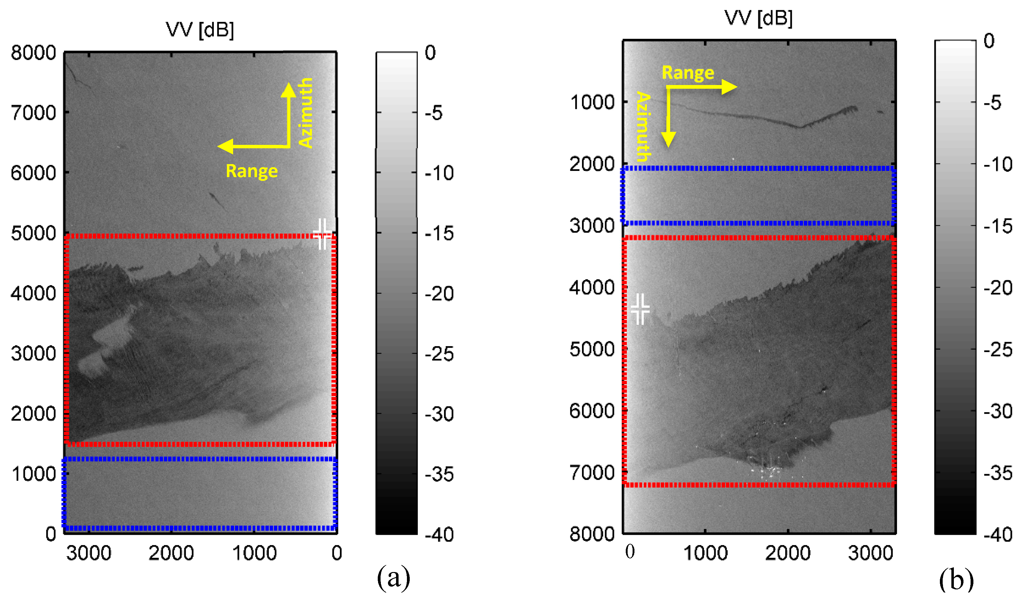
VV polarization UAVSAR images are shown in Figure 3. Figure 3a,b denote tracks 32,010 and 14,010, respectively. For reference, the bold crosses ╬ in these two images show a common point in the overlap region of the two swaths. The DWH oil rig is at the bottom of the spill area in Figure 3b, near radar coordinates (1800, 6400). The surface vessels and platforms near the DWH rig site are denoted by the tiny bright points in the water. Other surface vessels are indicated as isolated bright points elsewhere in the image, often with disturbed oil in their wake. Horizontal and vertical coordinates correspond to range and azimuth directions, respectively. The blue and red rectangles in Figure 3a,b are the oil free and oil-covered areas, as mentioned in the list of steps to retrieve the oil–water mixture ratio, respectively. They are used in the following analysis.

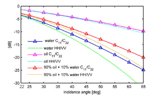
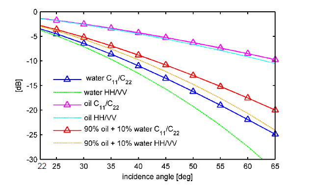
Figure 4 presents the variations of C₁₁/C₂₂ and HH/VV for oil spills and clean water areas from the DWH spill disaster with incidence angles indicated. The water and oil spill areas are the blue and red dotted - line rectangles in Figure 3, respectively. Both C₁₁/C₂₂ and HH/VV decrease with increasing incidence angles, when incidence angles are lower than 60°, for oil spill areas and oil-free water. 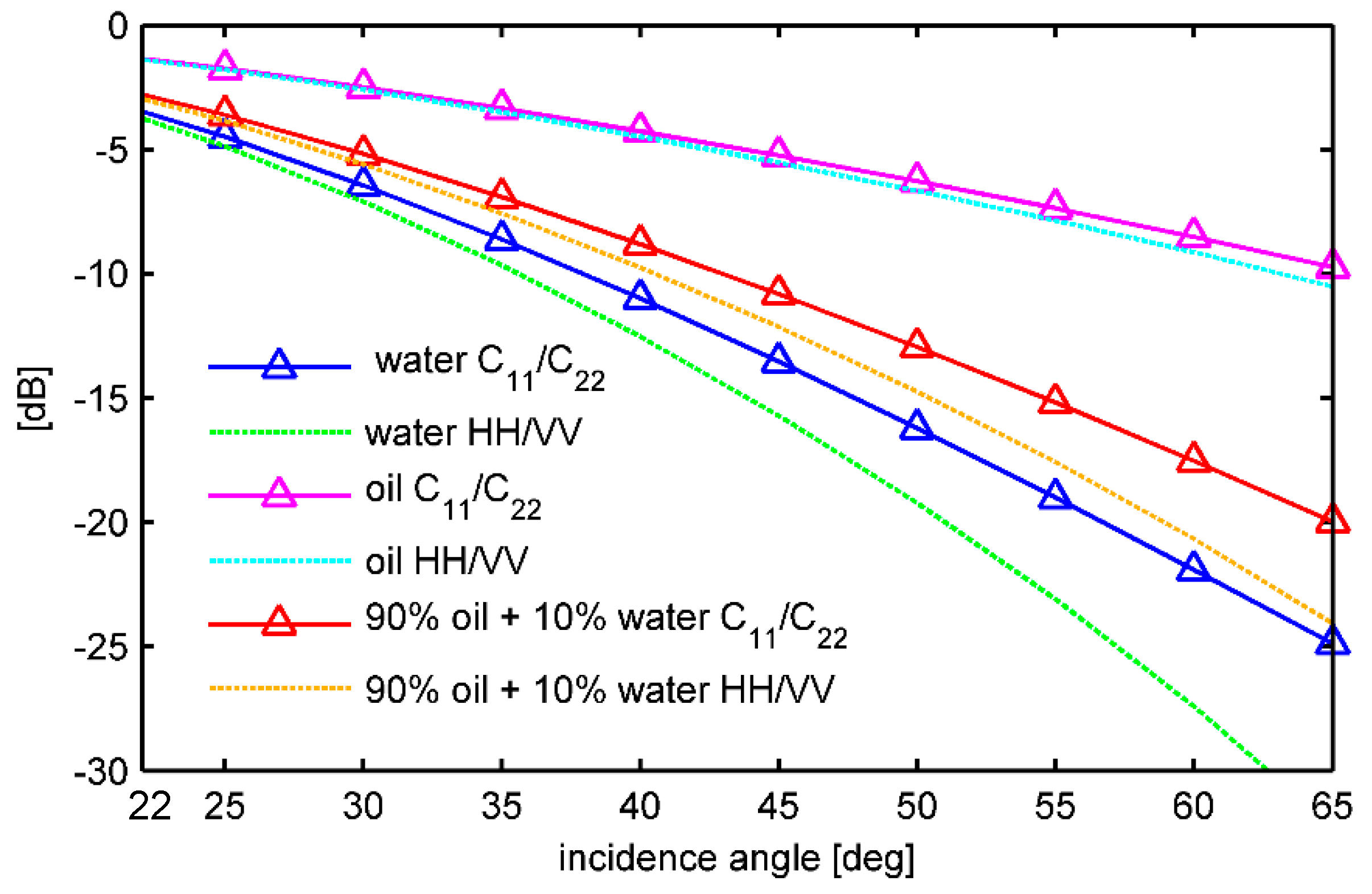The trends in Figure 4 for SAR observations are similar to trends in the theoretical results in Figure 1 when incidence angles are lower than 60°. The consistency of the theoretical and observation results demonstrates the potential applications of the theoretical model.

When incidence angles are larger than 60°, the variations are complicated, especially, for the oil-covered areas for C₁₁/C₂₂ and HH/VV; they first decrease then increase with increasing incidence angles. The similar increasing and decreasing of HH/VV for oil spill areas with incidence angles has also been shown in oil 2 of Figure 8 in [10]. Minchew et al. [10] attributed this behavior to the inhomogeneous distribution of the oil spill. [34,46,47] have pointed out the inhomogeneous properties noting that the “DWH polluted area includes oil slicks of different thicknesses, emulsified oil, weathered oil, oil/dispersant mixture, fresh oil, etc., the surface slick is very heterogeneous, including different kinds of surfactants.”

5. Results and Analysis

As mentioned in Section 4, before the mixture ratio of the oil spill can be calculated, we estimate the tilt of the Bragg scattering planes ψ and ζ by fitting the C₁₁/C₂₂ curve, using numerical optimization based on the tilted-Bragg scattering model for the oil-free areas, and assuming a dielectric constant of 80 − 70$\mathrm{i}$ for sea water. The RMS wave slopes, calculated as the RMS of ψ and ζ from the HP mode CP SAR data, are 10.73° and 9.24° for tracks 14,010 and 32,010, respectively. These values are close to the RMS wave slopes 9.07° and 13.35° obtained by the HH/VV ratio from original QP observations [10]. We obtain the ocean spectral density $W(·)$ in the oil-free area, by optimization fitting, using the estimated ocean surface wave slopes, ${\mathsf{\Gamma }}_{\mathrm{VV}}$, and ${\mathsf{\Gamma }}_{\mathrm{HV}}$ based on Equation (16). C₂₂ (VV) is used for the inversion because the values are larger than those of the C₁₁ (HH) data.

With ocean wave spectral density $W(·)$ and parameters $\psi ,\zeta$, ${\theta }_i$, ${\mathsf{\alpha }}_{\mathrm{HH}}$, ${\mathsf{\alpha }}_{\mathrm{vv}}$, ${\mathsf{\Gamma }}_{\mathrm{VV}}$, ${\mathsf{\Gamma }}_{\mathrm{HH}}$ and ${\mathsf{\Gamma }}_{\mathrm{HV}}$, we can obtain the elements of the HP covariance matrix C₁₁ and C₂₂ using numerical optimization following Equations (1), (13) and (16). 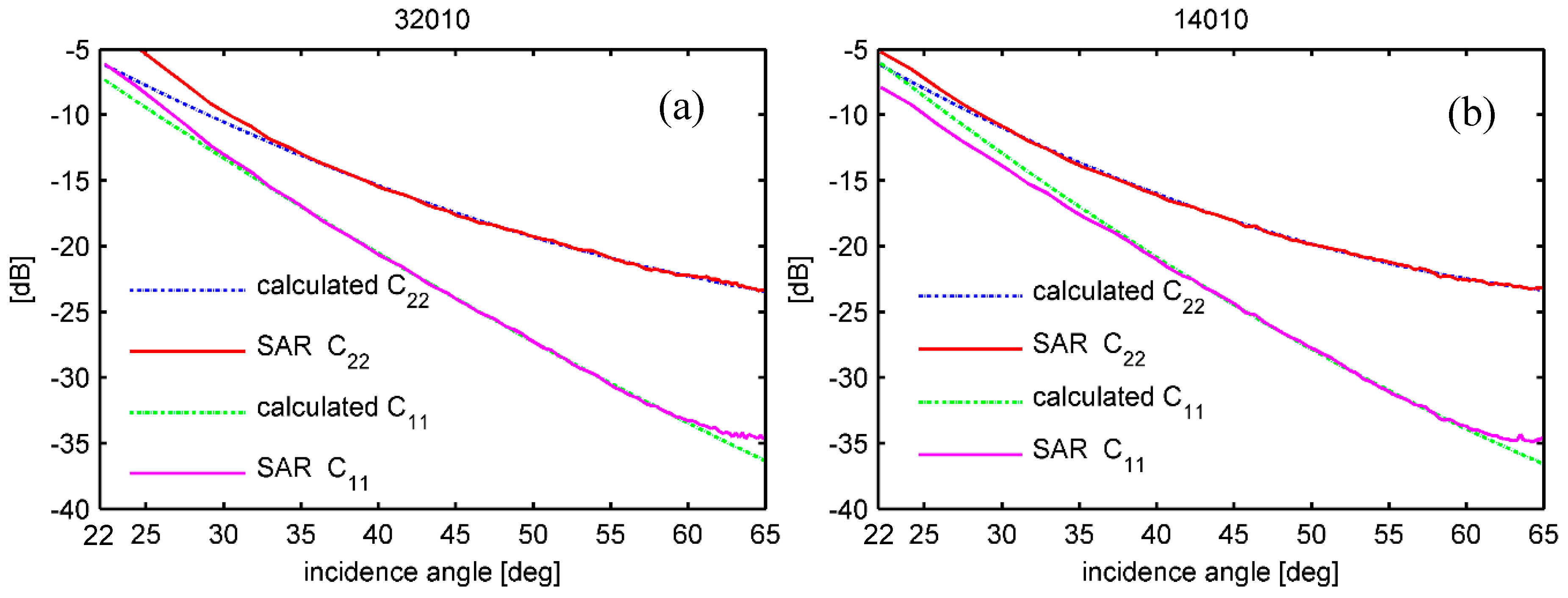Figure 5 compares the calculated C₁₁ and C₂₂ with those obtained from emulated CP SAR data directly. For both tracks 32,010 and 14,010, when the incidence angles are larger than 35°and less than 60°, the calculated values for C₁₁ and C₂₂ almost overlap those from the HP SAR observations.

All the above computations are performed for the oil-free (water) areas, indicated by the blue rectangles in Figure 3. The key parameters are related to the wave slope. The consistency of the calculated RMS wave slope, and the agreement of the elements of the HP covariance matrix obtained, using the proposed method, with those of the HP SAR observations, demonstrate the feasibility of the proposed methodology. The following calculation will be made for the oil-covered area to estimate the oil water mixture ratio using the ratio C₁₁/C₂₂, which decouples the effects of oil on the complex dielectric constant, from the effects of surface roughness.

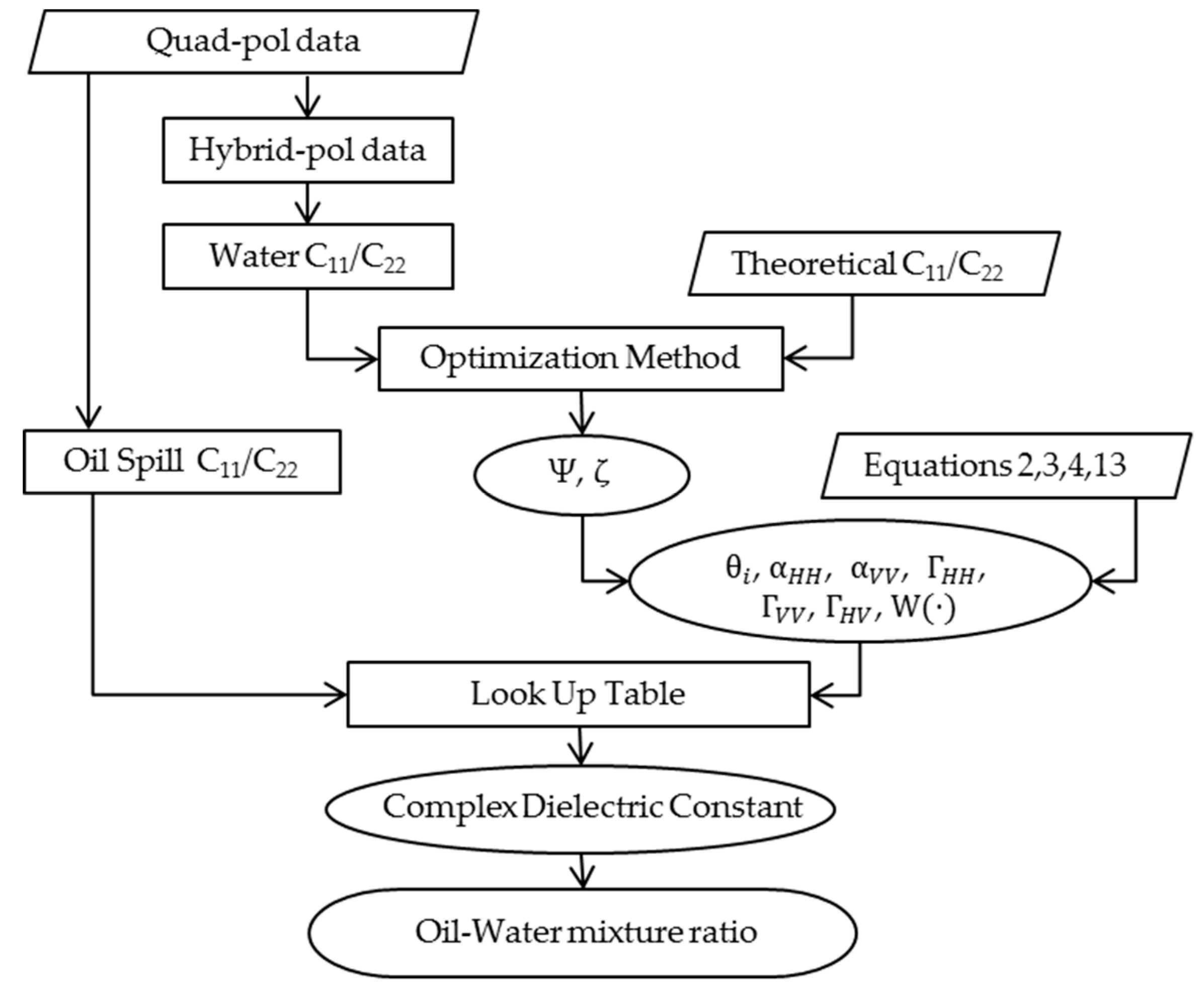
The oil–water mixture ratio look up table is established based on steps (6)–(7), using the slope angles ψ and ζ in the oil-free water area, substituting $\psi ,\zeta ,$ ${\epsilon }_r$ and ${\theta }_i$ into the relation $({\mathsf{\Gamma }}_{\mathrm{HH}}+{\mathsf{\Gamma }}_{\mathrm{HV}})/({\mathsf{\Gamma }}_{\mathrm{VV}}+{\mathsf{\Gamma }}_{\mathrm{HV}})$. Thus, the oil–water mixture ratio ${\mathsf{\epsilon }}_{\mathrm{r}}$ can be evaluated based on steps (8) and (9).

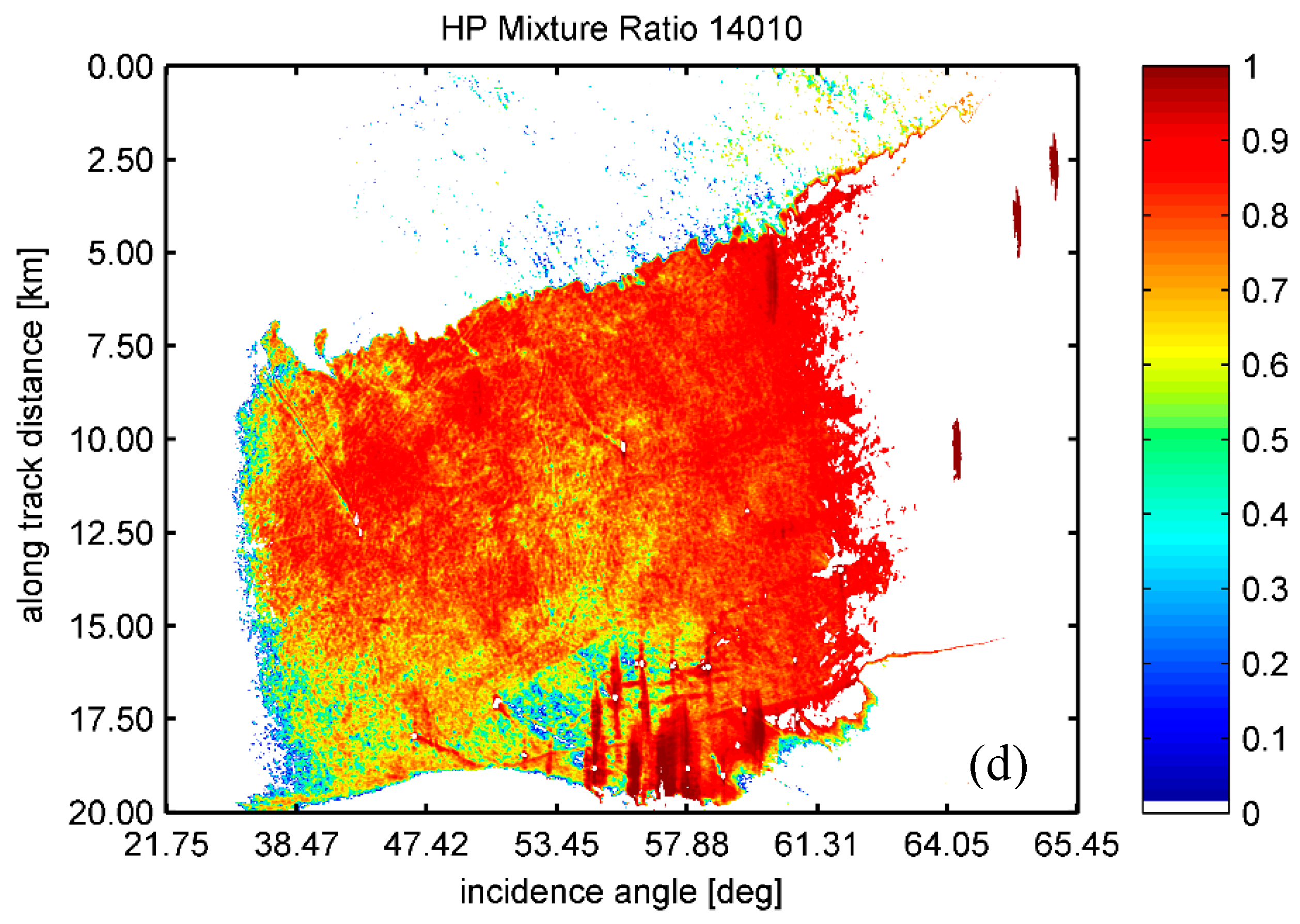
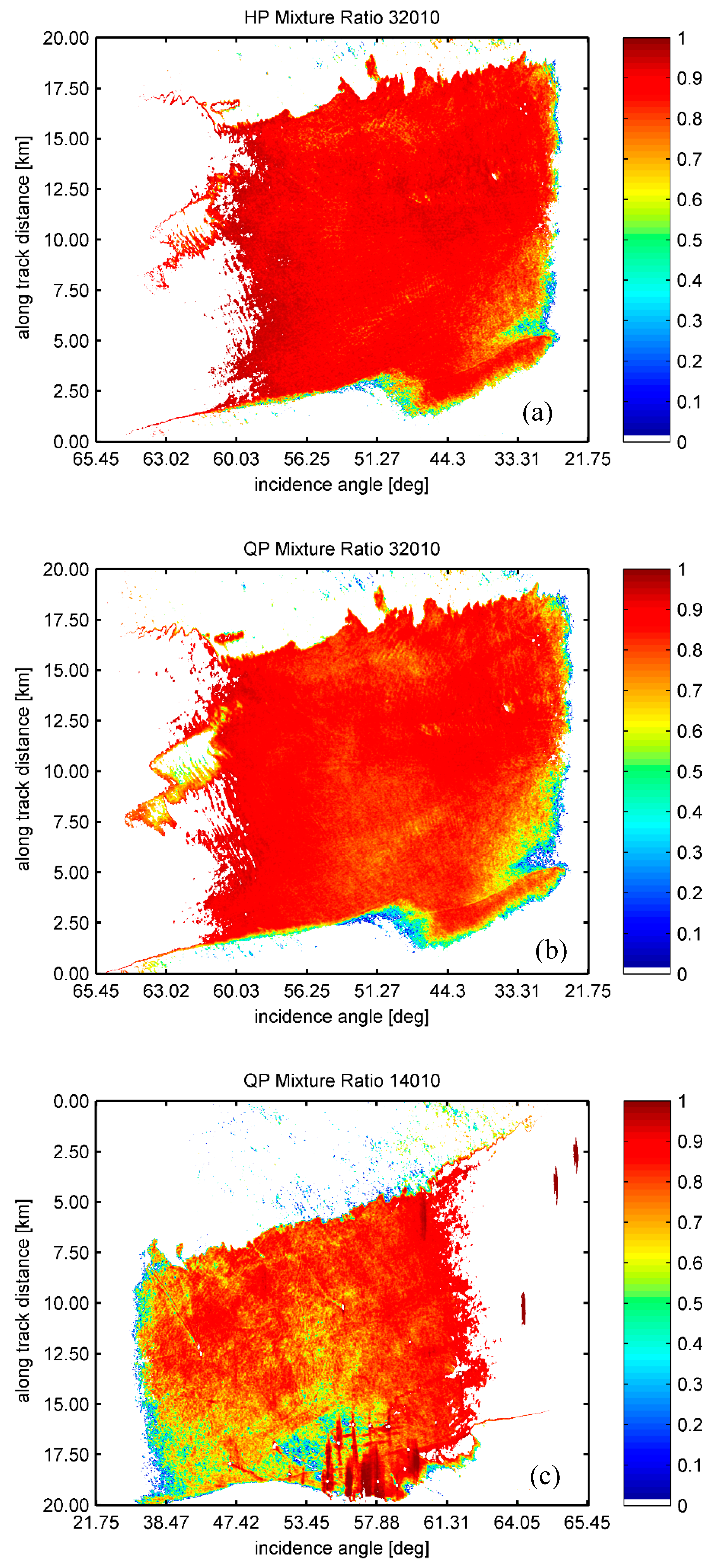
The spatial patterns of the mixture ratio of the oil spills denoted with red rectangles in Figure 3 are shown in Figure 6. Figure 6a,b are results for track 32,010 with QP and HP data, respectively, whereas Figure 6c,d are results for track 14,010, also with QP and HP data. The mixture ratios estimated with the proposed ratio C₁₁/C₂₂ from the HP data are comparable, in terms of their spatial patterns, with the evaluations from HH/VV from the QP observations. Consistency between the two methods is observed, especially for track 14,010. To make the comparison easy, the color scales in all panels are the same.

A slight overestimation in the mixture ratio from HP in track 32,010 can be observed in Figure 6a. The primary reason for the overestimation in these results is because of the inaccuracy of the wave slope angles and application of the same wave slope assumption in both oil spill areas and oil-free areas. This result may be also due to the entirety of the complicated mixing process of oil spills in DWH [46] and interactions between the oil and the waves [51]. Ocean waves typically have periods of less than a minute. During the acquisition of the SAR observations, the ocean waves imaged by SAR are therefore not strictly homogenous in space and time. Oil is known to mix with water through the actions of waves, wind and current; weathering and oil properties can change on timescales of hours to days due to the loss of volatiles, emulsification, entrainment of sediment, and other weathering processes [52]. The fate and transport of spilt oil depends on biological, chemical, physical and hydrodynamic processes, as well as processes such as spreading, evaporation, emulsification, dispersion, advection, photo-oxidation, biodegradation, dissolution, encapsulation and sedimentation, which take place simultaneously after an oil spill [11,34,51,53]. These processes are complex, sometimes self-competing and always simultaneous. The diversity and variability of oil spills requires different types of processing algorithms [54]. The tracks 32,010 and 14,010 have different locations, with 26 min difference in imaging times. Thus, these tracks may represent different stages in the oil spill aging processes. Minchew et al. [10] have suggested that the reason for the difference in the apparent oil–water mixture ratios between the two flight lines could indicate less complete mixing in track 14,010 which is closer to the DWH site. This point can be observed from the difference of the spatial patterns of the mixture ratios in Figure 6a,c. Overall, the mixture ratios for track 32,010 are higher than those of track 14,010. Till now, the characteristics of the different stages of oil spill development have not been taken into account in this study. Nonetheless, comparable results for both cases, with HH/VV and C₁₁/C₂₂ methods, highlight the utility of C₁₁/C₂₂ for estimates of oil spill mixture ratios.

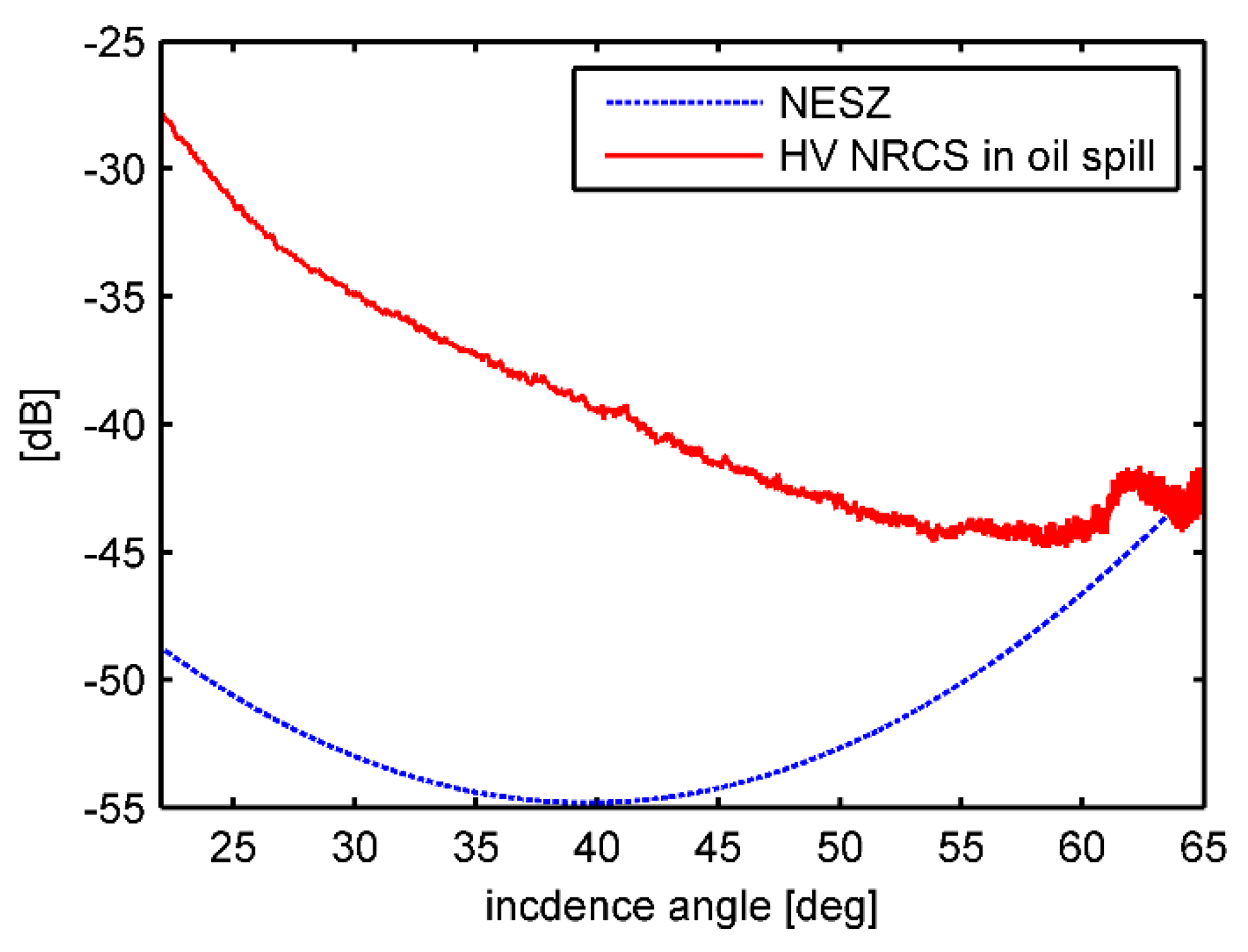
When the incidence angle is below approximately 26°, specular scattering is dominant for L band [10]. As a result, little information is available in these data that can characterize oil and water based on Bragg scattering. Data at high incidence angles are also considered to illustrate the NESZ influence [10]. The noise analysis has been shown in Figure 7 of [10], by plotting the backscattered signals and the estimated NESZ versus the incidence angle. Moreover, when simulating the HP data from the QP data, a 3-dB power loss is introduced due to $\sqrt{2}$ in Equation (12) [16]. In the worst scenario, noise contributes only a few percent to the total measured power at the high incidence angles. When NRCS values are close to, or lower than the noise floor, the mixture ratio cannot be estimated for high incidence angles. Thus, the mixture ratio is set to zero for lower and higher incidence angles. The reason for the former is that the area with lower incidence angle is dominated by specular scattering; the reason for the latter is that the NRCS of HV cannot reach 3 dB higher than the NESZ. The variation of NESZ and NRCS of HV of UAVSAR with the incidence angle are presented in Minchew et al. [10] and Fore et al. [50]. We provide that discussion in Appendix A.

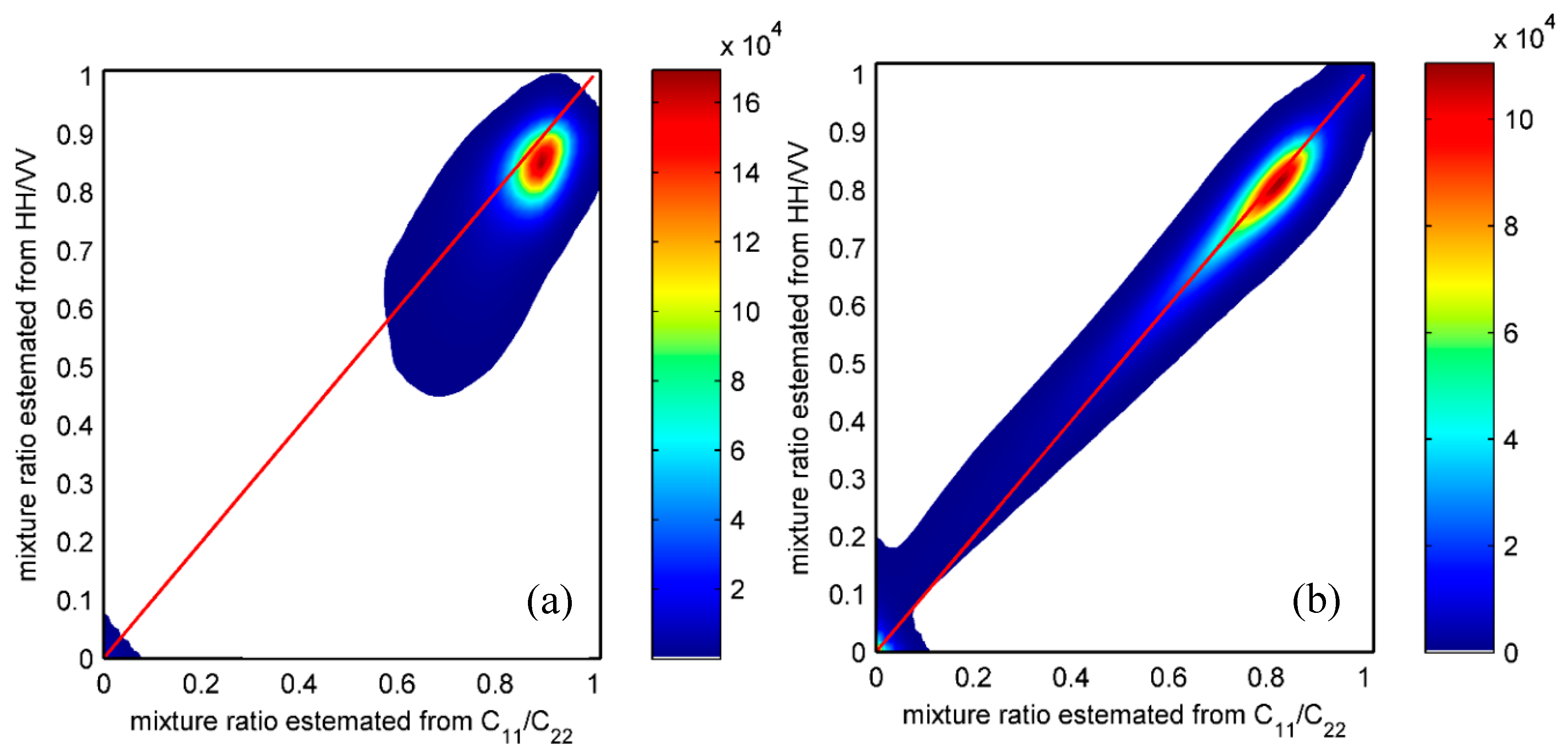
Scatter plots of the oil–water mixture ratio are shown in Figure 7 as suggested by C₁₁/C₂₂ from HP mode CP SAR data and compared with QP UAVSAR observations. Figure 7a,b denote cases 32,010 and 14,010, respectively. It is obvious that the mixture ratios for the two cases are different. In track 32,010, the values of most mixture ratios range from 0.7 to 0.9, and the pixels of the mixture ratio below 0.1 constitute only a small population. The reason for the location of the aggregation center with lower values is the small region of the open water area in Figure 6. There are almost no pixels with mixture ratios for the range from 0.1 to 0.4 for track 32,010, while the mixture ratio ranges from 0 to 1 for track 14,010. However, all the data are almost symmetrically distributed along the diagonal line for both cases. Thus, the scatter plots describe how well the derived mixture ratios from CP data match those derived from QP observations.

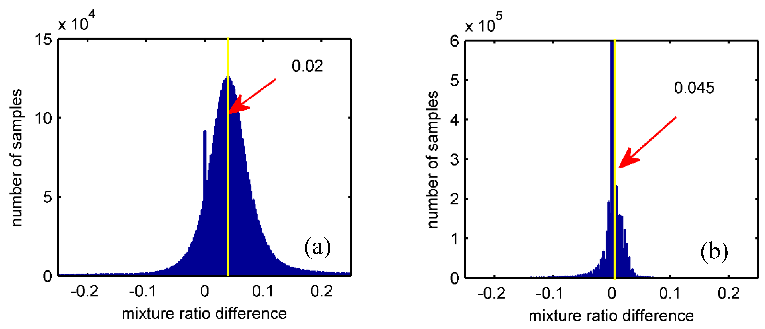
Moreover, mixing ratio estimates in Figure 6 and Figure 7 from C₁₁/C₂₂ are confirmed by histograms of the derived mixture ratio differences, displayed in Figure 8. The aim of Figure 8 is to demonstrate mixture ratio differences between QP and HP observations quantitatively. Variances result from estimates from HP mode SAR data, simulated from QP UAVSAR observations, and estimates from HH/VV based on quad-pol observations [31]. Figure 8a,b represent the tracks 32,010 and 14,010, respectively. The results from HP mode CP data display overall good agreement with those retrieved from quad-pol data with the HH/VV ratio. However, there is statistical overestimation for the values of the mixture ratio from the HP SAR data, which are denoted by the yellow line; the exact value is marked near the line in each case. As mentioned above, possible reasons for overestimation are: (a) our assumption of the same wave slope in the oil-free area and in the oil spill area, and (b) ignoring the complex variation of the oil spill and ocean waves as mentioned in the description of Figure 6. The statistical overestimation of track 32,010 is 0.02, while for track 14,010 the overestimation is 0.0045. The latter is one order of magnitude better than the former. The result is consistent with prior analysis. Statistically, the overestimation results are acceptable.

Statistical measures of the results are shown in

Table 1. Statistical results for mixture ratio.

Track	Bias	Correlation Coefficient	RMS Error
32,010	0.09	0.71	0.14
14,010	0.02	0.98	0.02

giving the bias, correlation coefficients and RMS error of the mixture ratio estimates from the original QP observations, relative to the estimates from the emulated HP mode CP SAR data. The standard deviation measures the distribution width. Positive values for the bias indicate that the mixture ratio estimates from the emulated HP data are larger than estimates from the original QP data. The results for track 32,010 are inferior to those for track 14,010, with bias and RMS error of 0.09 and 0.14, and correlation coefficient, 0.71. This represents a moderately positive correlation. However, track 14,010 has a better performance in terms of the mixture ratio estimation, with bias and RMS error of the derived mixture ratio of 0.02 and also 0.02, respectively, and a correlation coefficient of 0.98. The results suggest that the methodology proposed here with CP data provides a reliable way to estimate the oil–water mixture ratio.

6. Discussion

Based on Equations (8) and (15), the co-pol ratio from the original QP data and the diagonal elements ratio from the covariance matrix of CP data are related to frequency through the complex dielectric constant. Moreover, when oil mixes with the water at a high enough concentration and in a sufficiently thick (emulsified) layer to reduce the effective dielectric constant of the sea surface, the proposed methodology can be used. Alpers et al. [36] pointed out that in order for “the dielectric constant to have a non-negligible influence on the radar scattering, the oil layer must have a thickness exceeding 1/10 of the penetration depth.”

The penetration depth is defined as the depth at which the intensity of the radar signal inside the material falls off to 1/e (or about 37%) of its original value. The formula of penetration depth ${\delta }_p$ is given as [35,36]:

$${\delta }_p=\frac{c}{2\omega \left|imag\left(\sqrt{{\epsilon }_r}\right)\right|}$$

(17)

where ${\epsilon }_r$ is the complex dielectric constant of the medium, c represents the speed of light, ω is the angular frequency of the incident radiation and $imag$ indicates the imaginary component. Based on Equation (17), we knew that the penetration depth will variation with frequency and the complex dielectric constant. It should be noted ${\epsilon }_r$ of seawater is dependent of frequency [35]. However, Alpers et al. [36] assumed that ${\epsilon }_r$ does not change with the frequency, and thus the penetration depth will be proportion to the radar wavelength. Thus, the penetration depth of C-band is smaller than that of L-band for the same medium. Therefore, with respect to the penetration depth, we can safely draw the conclusion that the methodology proposed here can be easily applied to C-band observations.

The NESZ is another factor that should be taken into account. Oil spills dampen the power of the backscattered returning electromagnetic waves. The HV signal is ~10 dB below the HH and VV signal levels. Thus, having the HV signal above the noise floor is a key factor to determine whether the data can be used or not. In general, for the methodology in this paper to be valid, the ${\sigma }^{\mathrm{o}}$ values for the HH, VV and HV mode data must be above the noise level for both water and oil-covered areas. Moreover, the 3 dB power loss for simulation of the HP data from QP data should also be taken into account.

7. Conclusions

The HP CP SAR is a new SAR mode. RCM will be launched later in 2019 and will carry this kind of new SAR mode. The application of L-band HP mode CP SAR for oil–water mixture ratio estimation is explored in this paper. HP CP SAR data was emulated from high quality UAVSAR QP observations. The covariance matrix elements and diagonal element ratios C₁₁/C₂₂ from HP SAR are presented in this study to estimate the oil–water mixture ratio. The basic idea is that ocean wave spectra, which describe the roughness of the ocean surface, are the common factor in the C₁₁ and C₂₂ variables, which are the elements from the CP covariance matrix. Therefore, the ratio C₁₁/C₂₂ of these elements from the CP covariance matrix is independent of ocean surface roughness, and only depends on incidence angle, RMS wave slope and complex dielectric constants, based on the tilted Bragg scattering model [40]. Thus, the ratio C₁₁/C₂₂ from the HP CP SAR covariance matrix decouples the effects of oil on ocean surface roughness from the effects of the complex dielectric constant. These properties have similar characteristics to the ratio HH/VV, which has been used for evaluating the oil water mixture ratio [31,32,33]. This point was confirmed by the similar trend in variations between the UAVSAR observations and the theoretical model results. Thus, we suggest that there is potential for C₁₁/C₂₂ from the HP mode CP SAR data for estimation of the oil–water mixture ratio.

The slope angles ψ and ζ obtained from HP data are close to those obtained from QP data. Meanwhile, the C₁₁ and C₂₂ calculated with wave spectra density, incidence angle and slope angles are consistent with those from the UAVSAR QP data. Moreover, it is very encouraging that the oil–water mixture ratio is in overall agreement for the results obtained from CP data with those obtained from QP data. Despite the good overall agreement, systematic overestimations and regionally dependent deviations are clearly visible. These may be due to the complexity, diversity and variability of oil spills and ocean waves. Although not applicable for quantitative assessment of the influences of such factors, the proposed C₁₁/C₂₂ from HP mode SAR data has demonstrated a potential application for estimation of the oil–water mixture ratio for oil spills on the ocean surface.

As mentioned previously, the NESZ is an important factor which should be taken into account for the damping effect of oil spill. Moreover, extensions of the method to other cases need further study because the DWH spill disaster represents a situation unlike any previous event. The measurements in NORSE2015 maybe good cases.

References

1. Schuler, D.L.; Lee, J.S. Mapping ocean surface features using biogenic slick-fields and SAR polarimetric decomposition technique. IEEE Proc. Radar Sonar Navig. 2006, 153, 260–270. [Google Scholar] [CrossRef]
2. Migliaccio, M.; Gambardella, A.; Tranfaglia, M. SAR polarimetry to observe oil spills. IEEE Trans. Geosci. Remote Sens. 2007, 45, 506–511. [Google Scholar] [CrossRef]
3. Nunziata, F.; Gambardella, F.; Migliaccio, M. On the Mueller scattering matrix for SAR sea oil slick observation. IEEE Geosci. Remote Sens. Lett. 2008, 5, 691–695. [Google Scholar] [CrossRef]
4. Ramsey, E., III; Rangoonwala, A.; Suzuoki, Y.; Jones, C.E. Oil Detection in a Coastal Marsh with Polarimetric Synthetic Aperture Radar (SAR). Remote Sens. 2011, 3, 2630–2662. [Google Scholar] [CrossRef]
5. Migliaccio, M.; Nunziata, F.; Montuori, A.; Li, X.; Pichel, W.G. A multi-frequency polarimetric SAR processing chain to observe oil fields in the Gulf of Mexico. IEEE Trans. Geosci. Remote Sens. 2011, 49, 4729–4737. [Google Scholar] [CrossRef]
6. Zhang, B.; Perrie, W.; Li, X.; Pichel, W.G. Mapping sea surface oil slicks using RADARSAT-2 quad-polarization SAR image. Geophys. Res. Lett. 2011, 38, L10602. [Google Scholar] [CrossRef]
7. Skrunes, S.; Brekke, C.; Eltoft, T. Characterization of marine surface slicks by Radarsat-2 multipolarization features. IEEE Trans. Geosci. Remote Sens. 2014, 52, 5302–5319. [Google Scholar] [CrossRef]
8. Song, D.; Ding, Y.; Li, X.; Zhang, B.; Xu, M. Ocean oil spill classification with RADARSAT-2 SAR based on an optimized wavelet neural network. Remote Sens. 2017, 9, 799. [Google Scholar] [CrossRef]
9. Skrunes, S.; Brekke, C.; Eltoft, T.; Kudryavtsev, V. Comparing near-coincident C- and X-band SAR acquisitions of marine oil spills. IEEE Trans. Geosci. Remote Sens. 2015, 53, 1958–1975. [Google Scholar] [CrossRef]
10. Minchew, B.; Jones, C.; Holt, B. Polarimetric analysis of backscatter from the Deepwater Horizon oil spill using L-band synthetic aperture radar. IEEE Trans. Geosci. Remote Sens. 2012, 99, 1–19. [Google Scholar]
11. Li, H.; Perrie, W.; He, Y.; Wu, J.; Luo, X. Analysis of the polarimetric SAR scattering properties of oil-covered waters. IEEE J. Sel. Top. App. Earth Obs. Remote Sens. 2014, 99, 1–9. [Google Scholar] [CrossRef]
12. Migliaccio, M.; Nunziata, F.; Buono, A. SAR polarimetry for sea oil slick observation. Int. J. Remote Sens. 2015, 36, 3243–3273. [Google Scholar] [CrossRef]
13. Ivonin, D.V.; Skrunes, S.; Brekke, C.; Ivanov, A.Y. Interpreting sea surface slicks on the basis of the normalized radar cross-section model using RADARSAT-2 copolarization dual-channel SAR images. Geophys. Res. Lett. 2016, 43, 2748–2757. [Google Scholar] [CrossRef]
14. Hansen, M.W.; Kudryavtsev, V.; Chapron, B.; Brekke, C.; Johannessen, J.A. Wave Breaking in Slicks: Impacts on C-Band Quad-Polarized SAR Measurements. IEEE J. Sel. Top. App. Earth Obs. Remote Sens. 2016, 9, 4929–4940. [Google Scholar] [CrossRef]
15. Souyris, J.-C.; Imbo, P.; Fjortoft, R.; Mingot, S.; Lee, J.-S. Compact polarimetry based on symmetry properties of geophysical media: The π/4 mode. IEEE Trans. Geosci. Remote Sens. 2005, 43, 634–646. [Google Scholar] [CrossRef]
16. Raney, R.K. Hybrid-Polarity SAR architecture. IEEE Trans. Geosci. Remote Sens. 2007, 45, 3397–3404. [Google Scholar] [CrossRef]
17. Brekke, C.; Jones, C.E.; Skrunes, S.; Holt, B.; Espeseth, M.; Eltoft, T. Cross-correlation between polarization channels in SAR imagery over oceanographic features. IEEE Geosci. Remote Sens. Lett. 2016, 13, 997–1001. [Google Scholar] [CrossRef]
18. Brekke, C.; Skrunes, S.; Espeseth, M. Oil spill dispersion in full-polarimetric and hybrid-polarity SAR. IEEE Int. Geosci. Remote Sens. Symp. 2017. [Google Scholar] [CrossRef]
19. Espeseth, M.M.; Skrunes, S.; Jones, C.E.; Brekke, C.; Holt, B.; Doulgeris, A.P. Analysis of evolving oil spills in full-polarimetric and hybrid-polarity SAR. IEEE Trans. Geosci. Remote Sens. 2017, 55, 4190–4210. [Google Scholar] [CrossRef]
20. Lingenahalli, J.V.K.; Kishore J., K.; Kesava, P. Unsupervised classification based on decomposition of RISAT-1 images for oil spill detection. In Proceedings of the 2013 International Conference on Advances in Computing, Communications and Informatics (ICACCI), Mysore, India, 22–25 August 2013. [Google Scholar] [CrossRef]
21. Hari-Priya, S.; Jayasri, P.V.; Sita-Kumari, E.V.S.; Prasad, A.V.V. On the estimation of polarimetric parameters for oil slick feature detection from hybrid pol and derived pseudo quad-pol SAR data. Int. Arch. Photogramm. Remote Sens. Spat. Inf. Sci 2018, XLII-5, 629–635. [Google Scholar] [CrossRef]
22. Shirvany, R.; Chabert, M.; Tourneret, J.-Y. Ship and oil-spill detection using the degree of polarization in linear and hybrid/compact dual-pol SAR. IEEE J. Sel. Topics Appl. Earth Observ. Remote Sens. 2012, 5, 885–892. [Google Scholar] [CrossRef]
23. Salberg, A.-B.; Rudjord, O.; Solberg, A.H.S. Oil spill detection in hybrid-polarimetric SAR images. IEEE Trans. Geosci. Remote Sens. 2014, 52, 6521–6533. [Google Scholar] [CrossRef]
24. Nunziata, F.; Migliaccrio, M.; Li, X. Sea oil slick observation using hybrid-polarity SAR architecture. IEEE J. Ocean. Eng. 2015, 40, 426–440. [Google Scholar] [CrossRef]
25. Li, H.; Perrie, W.; Zhou, Y.; He, Y. Oil spill detection on the ocean surface using hybrid polarimetric SAR imagery. Sci. China 2015, 59, 249–257. [Google Scholar] [CrossRef]
26. Buono, A.; Nunziata, F.; Migliaccio, M.; Li, X. Polarimetric Analysis of Compact-Polarimetry SAR Architectures for Sea Oil Slick Observation. IEEE Trans. Geosci. Remote Sens. 2016, 54, 5862–5874. [Google Scholar] [CrossRef]
27. Buono, A.; Nunziata, F.; Migliaccio, M. Polarimetric Analysis of Full and Compact Polarimetric SAR Features Over the Sea Surface. IEEE Geosci. Remote Sens. Lett. 2016, 13, 1527–1531. [Google Scholar] [CrossRef]
28. Salberg, A.; Larsen, S. Classification of Ocean Surface Slicks in Simulated Hybrid-Polarimetric SAR Data. IEEE Trans. Geosci. Remote Sens. 2018, 56, 7062–7073. [Google Scholar] [CrossRef]
29. Yin, J.; Yang, J.; Zhou, Z.; Song, J. The Extended Bragg Scattering Model-Based Method for Ship and Oil-Spill Observation Using Compact Polarimetric SAR. IEEE J. Sel. Topics Appl. Earth Observ. Remote Sens. 2015. [Google Scholar] [CrossRef]
30. Fingas, M. The challenges of remotely measuring oil slick thickness. Remote Sens. 2018. [Google Scholar] [CrossRef]
31. Minchew, B. Determining the mixing of oil and sea water using polarimetric synthetic aperture radar. Geophys. Res. Lett. 2012, 39. [Google Scholar] [CrossRef]
32. Angelliaume, S.; Boisot, O.; Guérin, C.A. Dual-polarized L-Band SAR Imagery for Temporal Monitoring of Marine Oil Slick Concentration. Remote Sens. 2018, 10, 1012. [Google Scholar] [CrossRef]
33. Boisot, O.; Angelliaume, S.; Guérin, C.-A. Marine Oil Slicks Quantification From L-band Dual-Polarization SAR Imagery. IEEE Trans. Geosci. Remote Sens. 2018. [Google Scholar] [CrossRef]
34. Nunziata, F.; Macedo, C.R.; Buono, A.; Velotto, D.; Migliaccio, M. On the analysis of a time series of X–band TerraSAR–X SAR imagery over oil seepages. Int. J. Remote Sens. 2018. [Google Scholar] [CrossRef]
35. Brekke, C.; Holt, B.; Jones, C.; Skrunes, S. Discrimination of oil spills from newly formed sea ice by synthetic aperture radar. Remote Sens. Environ. 2014, 145, 11–14. [Google Scholar]
36. Alpers, W.; Holt, B.; Zeng, K. Oil spill detection by imaging radars: Challenges and pitfalls. Remote Sens. Environ. 2017, 201, 133–147. [Google Scholar] [CrossRef]
37. Li, H.; Perrie, W.; Li, Q.; Hou, Y. Estimation of Melt Pond Fractions on First Year Sea Ice Using Compact Polarization SAR. J. Geophys. Res. 2017. [Google Scholar] [CrossRef]
38. Collins, M.J.; Denbina, M.; Minchew, B.; Jones, C.E.; Holt, B. On the Use of Simulated Airborne Compact Polarimetric SAR for Characterizing Oil–Water Mixing of the Deepwater Horizon Oil Spill. IEEE J. Sel. Top. App. Earth Obs. Remote Sens. 2015, 8. [Google Scholar] [CrossRef]
39. Raney, R.K. Comparing Compact and Quadrature Polarimetric SAR Performance. IEEE Geosci. Remote Sens. Lett. 2016, 13, 861–864. [Google Scholar] [CrossRef]
40. Valenzuela, G. Theories for the interaction of electromagnetic and ocean waves—A review. Bound.-Layer Meteorol. 1978, 13, 61–85. [Google Scholar] [CrossRef]
41. Scharien, R.K.; Hochheim, K.; Landy, J.; Barber, D.G. First-year sea ice melt pond fraction estimation from dual-polarisation C-band SAR- Part 2: Scaling in situ to Radarsat-2. Cryosphere 2014, 8, 2163–2176. [Google Scholar] [CrossRef]
42. Hulst, H.C.; Hulst, C.V.D. Light Scattering by Small Particles; Courier Corporation: Dover Publications, Inc.: New York, NY, USA, 1957. [Google Scholar]
43. Friiso, T.; Schildberg, Y.; Rambeau, O.; Tjomsland, T.; Fordedal, H.; Sjoblom, J. Complex permittivity of crude oil and solutions of heavy crude oil fractions. J. Dispersion Sci. Technol. 1998, 19, 93–126. [Google Scholar] [CrossRef]
44. Kudryavtsev, V.N.; Chapron, B.; Myasoedov, A.G.; Collard, F.; Johannessen, J.A. On dual co-polarized SAR measurements of the ocean surface. IEEE Trans. Geosci. Remote Sens. Lett. 2013, 10, 761–765. [Google Scholar] [CrossRef]
45. Wright, J. A new model for sea clutter. IEEE Trans. Antennas Propag. 1968, AP-16, 217–223. [Google Scholar] [CrossRef]
46. Nunziata, F.; Buono, A.; Migliaccio, M. COSMO–SkyMed Synthetic Aperture Radar data to observe the deep water horizon oil spill. Sustainability 2018, 10, 3599. [Google Scholar] [CrossRef]
47. Migliaccio, M.; Nunziata, F. On the exploitation of polarimetric SAR data to map damping properties of the Deepwater Horizon oil spill. Int. J. Remote Sens. 2014, 35, 10–3499. [Google Scholar] [CrossRef]
48. Garcia-Pineda, O.; Holmes, J.; Rissing, M.; Jones, R.; Wobus, C.; Svejkovsky, J.; Hess, M. Detection of oil near shorelines during the Deepwater Horizon oil spill using Synthetic Aperture Radar (SAR). Remote Sens. 2017, 9, 567. [Google Scholar] [CrossRef]
49. Vilcáez, J.; Li, L.; Hubbard, S.S. A new model for the biodegradation kinetics of oil droplets: Application to the Deepwater Horizon oil spill in the Gulf of Mexico. Geochem. Trans. 2013, 14, 1–14. [Google Scholar]
50. Fore, A.G.; Chapman, B.D.; Hawkins, B.P.; Hensey, S.; Jone, C.E.; Michel, T.R.; Muellerschoen, R.J. UAVSAR Polarimetric Calibration. IEEE Trans. Geosci. Remote Sens. 2015, 53, 3481–3491. [Google Scholar] [CrossRef]
51. Leifer, I.; Lehr, W.J.; Simecek-Beatty, D.; Bradley, E.; Clark, R.; Dennison, P.; Hu, Y.; Matheson, S.; Jones, C.E.; Holt, B.; et al. State of the art satellite and airborne marine oil spill remote sensing: Application to the BP Deepwater Horizon oil spill. Remote Sens. Environ. 2012, 124, 185–209. [Google Scholar] [CrossRef]
52. National Research Council. Oil in the Sea III: Inputs, Fates, and Effects; National Academies Press: Washington, DC, USA, 2003. [Google Scholar]
53. Afenyo, M.; Veitch, B.; Khan, F. A state-of-the-art review of fate and transport of oil spills in open and ice-covered water. J. Ocean Eng. 2016, 119, 233–248. [Google Scholar] [CrossRef]
54. Topouzelis, K.; Singha, S. Oil spill detection: Past and future, trends. In Proceedings of the ESA Living Planet Symposium 2016, Prague, Czech Republic, 9–13 May 2016. [Google Scholar]
55. Younis, M.; Huber, S.; Patyuchenko, A.; Bordoni, F.; Krieger, G. Performance comparison of reflector- and planar-antenna based digital beam-forming SAR. Int. J. Antennas Propag. 2009. [Google Scholar] [CrossRef]
Figure 1. The variation of HH/VV and C11/C22 with incidence angles for the complex dielectric constants of crude oil, oil spill and sea water. The values of HH/VV with different dielectric constants are represented with different colored dotted lines ……, and for C11/C22 with different dielectric constants, by different colors solid lines with triangles Remotesensing 11 00816 i001.
Remotesensing 11 00816 g001
Figure 2. Flowchart of the proposed methodology. The elliptical and rounded boxes represent the intermediate and final outputs, respectively. The parallelogram and rectangle boxes denote inputs and processing steps, respectively.
Remotesensing 11 00816 g002
Figure 3. The VV normalized radar cross section (NRCS) images of tracks (a) 32,010, (b) 14,010. The red and blue rectangles segment the oil spill and oil free water areas, respectively. The bold white crosses ╬ in these two images show a common point in the overlap region of the two swaths. The tiny white spots in (b) around azimuth line 6500 and midrange are surface vessels and platforms at the Deep Water Horizon (DWH) site. The yellow lines denote the azimuth and range directions.
Remotesensing 11 00816 g003
Figure 4. C11/C22 and HH/VV vs. incidence angle for oil-free and oil spill areas in the DWH spill disaster area for tracks (a) 32,010 and (b) 14,010. The water and oil spill areas are the blue and red dotted-line rectangles in Figure 3, respectively.
Remotesensing 11 00816 g004
Figure 5. Comparisons of the calculated C11 and C22 with those from emulated compact polarization synthetic aperture radar (CP SAR) observations for Tracks 32,010 (a) and 14,010 (b). The water areas are indicated by the blue dotted-line rectangles in Figure 3.
Remotesensing 11 00816 g005
Figure 6. The mixture ratio. (a,b) for track 32,010 from quad-polarization (QP) and hybrid-polarized (HP) data; (c,d) for track 14,010 from QP and HP data, respectively.
Remotesensing 11 00816 g006aRemotesensing 11 00816 g006b
Figure 7. Scatter plots of oil–water mixture ratio estimated using C11/C22 from HP data (x-axis) with those estimated from QP Uninhabited Aerial Vehicle SAR (UAVSAR) observations (y-axis): (a) track 32,010 (b) track 14,010. Color bar denotes data number density and the diagonal line indicates perfectly matching data.
Remotesensing 11 00816 g007
Figure 8. Histograms (y-axis) of derived mixture ratio differences between the results from HP mode CP data and UAVSAR quad-pol observations with HH/VV ratio on the x-axis. (a,b) denote the differences for tracks 32,010 and 14,010, respectively. The yellow line denotes the statistical overestimations and the exact values are marked near the line, in each case.
Remotesensing 11 00816 g008