Goaf Locating Based on InSAR and Probability Integration Method

Abstract

Mining goafs can cause many hazards, such as burst water, spontaneous combustion of coal seams, surface collapse, etc. In this paper, a feature-points-based method for the efficient location of mining goafs is proposed. Different interferometric synthetic aperture radar (DInSAR) is used to monitor the subsidence basin caused by mining. Using the principles of the probability integral method (PIM), the inflection points and the boundary points of the basin monitored by DInSAR are determined and used as feature points to locate the goaf. In this paper, the necessity of locating goafs and the traditional methods used for this task are discussed first. Then, the results of verifying the proposed method by both a simulation experiment and real data experiment are presented. Six RADARSAT-2 images from 13th October 2015 to 5th March 2016 were used to acquire the subsidence basin caused by the 15235 working faces of the Jiulong mining area. The average relative errors of the simulation experiment and real data experiment were about 6.43% and 12.59%, respectively. The average absolute errors of the simulation experiment and real data experiment were about 28 m and 38 m, respectively. In the final part of this paper, the error sources are discussed to illustrate the factors that can affect the location result.

1. Introduction

Coal production and coal consumption are extensive in China, as coal is the country’s main energy source. According to the National Energy Administration (http://www.nea.gov.cn), coal production capacity in China is increasing every year. As of the end of June 2017, the national total coal production capacity was 3.41 billion tons/year, and it had increased to 3.49 billion tons/year by June 2018. It is estimated that by 2020, the national energy consumption will still include more than 60% coal. In 2017, the world’s coal production was 7.73 billion tons, of which China accounted for 45.6%.

Such large-scale mining results in many goafs. Many of them are recorded, but because of the existence of illegal mining and loss of records, there are many unknown goafs hidden underground with the potential to cause many disasters. Mining under the original goaf activates the overlying rock, which can then lead to secondary disasters, such as ground collapse [1,2]. Mining activities next to goafs can lead to falling roofs, aquifer rupture, and other hazards that can endanger the safety of underground workers [3]. The sudden collapse of a goaf will affect agricultural production, as well as result in damage to the buildings above, landslides, and other geological disasters that endanger people’s lives [4]. Traditional methods to monitor goafs are mainly geophysical, including temperature measurement, the magnetic method, resistivity measurement, carbon monoxide measurement, the transient electromagnetic method, the geological radar detection method, and radioactive radon detection [5]. These methods are time-consuming, inefficient, and easily disrupted. Therefore, accurate and efficient goaf monitoring technology has great social and engineering application value.

As a new deformation monitoring technology, the interferometric synthetic aperture radar (InSAR) has been widely studied and applied in many fields, such as mining area subsidence [6,7,8], urban subsidence [9,10,11], volcanic activities [12,13], and glacier drift [14]. InSAR technology has unique advantages in discriminating the deformation of mining areas. Firstly, InSAR can monitor a large area with high precision. Secondly, compared with conventional goaf detection methods, the economic and labor costs of InSAR are very low. Moreover, InSAR has abundant archival data, so mining activities in the past can still be identified.

As far as we know, there have been few studies on locating goafs by InSAR. Li et al. [15] used DInSAR technology to monitor surface deformation. The sinking areas were analyzed through field investigations to determine whether there were goafs. This method can identify mining goafs accurately, but it has a high economic cost and is labor-intensive. Hu et al. [16] proposed a method using DInSAR monitoring results to calculate the center coordinates of the mining area. This method has lower economic and labor costs, but it cannot obtain the boundaries of goafs. Besides this, the method simplifies the goaf by treating it as horizontal, so the result is not reliable when the coal seam is on an incline. Xia et al. [17] used DInSAR to detect surface deformation; then, according to the shape of the basin, GIS was used to determine whether the deformation was caused by mining. This method can detect mining goafs without manual intervention. However, like the method proposed by Hu et al. [16], it can only offer the coordinates of the goaf instead of all of the information about the goaf, such as the length, height, and position of the boundaries. Yang et al. [18] first obtained the surface subsidence basin by DInSAR technology, established the functional relationship between the surface subsidence basin and the parameters of the probability integral method (PIM), and then searched for the optimal solution through a genetic algorithm and annealing algorithm to invert the shape of the underground goaf. This method can determine the boundary and depth of the goaf and does not need fieldwork. However, a large number of comparative experiments are needed to determine the parameters of the two nonlinear inversion models, and it is difficult to meet such requirements in engineering applications. Moreover, the relationship between the inverted parameters of the PIM is not taken into account, so it may not reflect the real situation.

According to the above research, the key problem in locating goafs by DInSAR is the need to establish a proper and reliable relational model between the basin and the goaf. The PIM, a method to predict surface deformation caused by mining, has a long history and is based on the stochastic medium theory [19]. After nearly fifty years of research by technicians, it has matured and become the most widely used method for prediction [20]. It also has been proved to be a dependable model when used for InSAR monitoring [21,22] and goaf locating [18].

In this study, we used DInSAR and the PIM to locate a goaf in a mining area. As stated in the literature [18], DInSAR is used to obtain the surface subsidence, and the PIM is a relational model between the subsidence basin and the boundaries and depth of a goaf. According to the principle of the PIM, we located the goaf using the feature points of the basin. Then, the reliability of this method was verified by simulation experiments and a real data experiment.

2. Experimental Principle

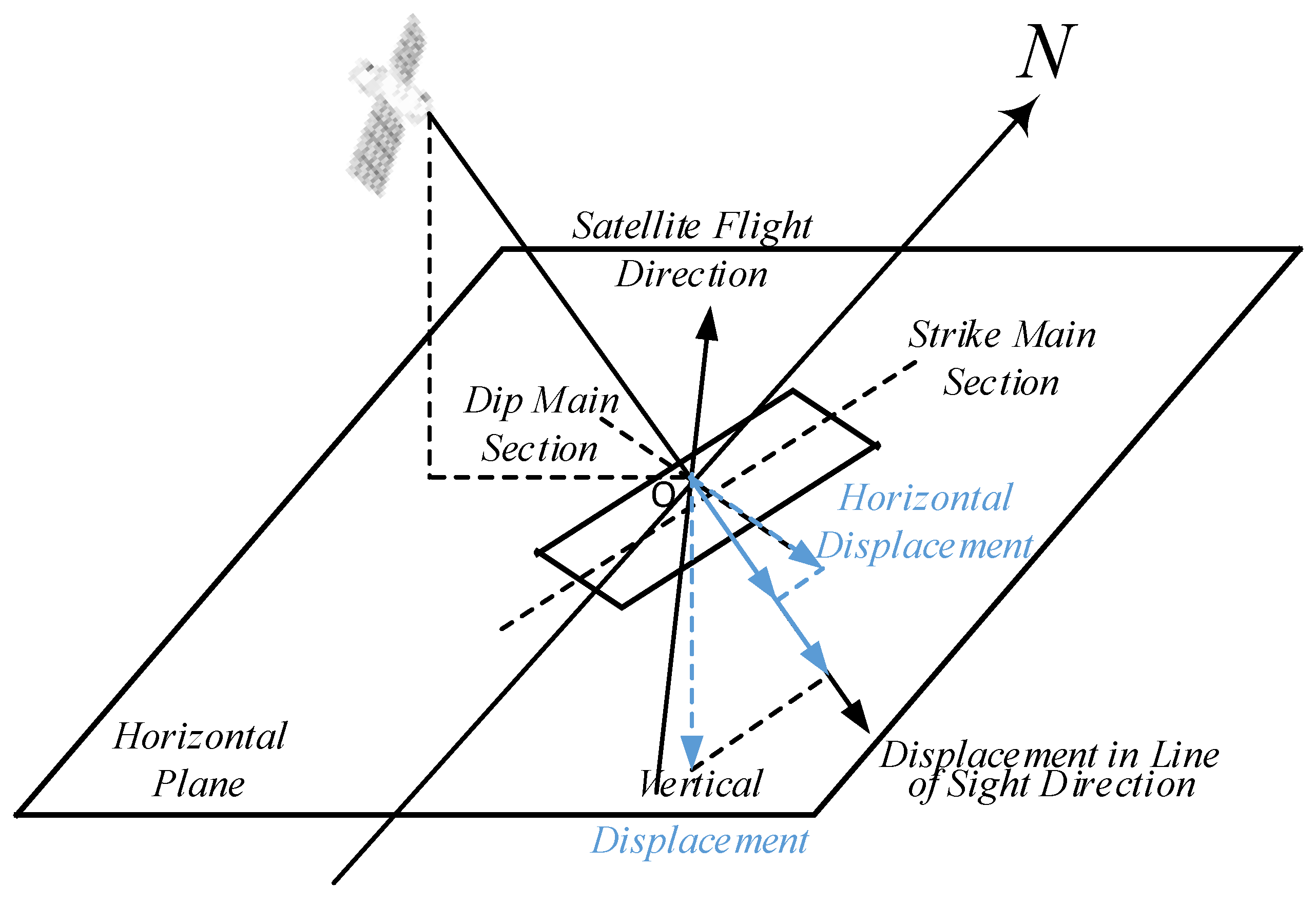
2.1. DInSAR Technology

DInSAR uses the phase information of SAR complex images to identify land surface deformation. An interferogram can be obtained by multiplying two SAR images by a conjugate. In the interference fringe pattern of two images, the interferometric phase $\phi$ is mainly composed of the following parts:

$$\phi =\omega ({\phi }_{top}+{\phi }_{flt}+{\phi }_{def}+{\phi }_{atm}+{\phi }_{noise}),$$

(1)

where $\omega (·)$ is the wrap operator; ${\phi }_{top}$ is the phase caused by the terrain, which can be removed by external digital elevation model (DEM) simulation; ${\phi }_{flt}$ is the flat phase, which can be removed by a precise baseline estimate; ${\phi }_{def}$ is the phase caused by the surface deformation in the line-of-sight (LOS) direction; ${\phi }_{atm}$ is the phase caused by atmospheric delay. By stacking the interferograms, the signal-to-noise ratio (SNR) of the deformation information can be improved, and the noise of atmospheric interference can be weakened, so the influence of the atmospheric delay can be reduced [23]. The parameter ${\phi }_{noise}$ is the noise phase and can be suppressed by low-pass filtering; then, the real phase is restored by the minimum cost flow method to obtain the surface deformation [24].

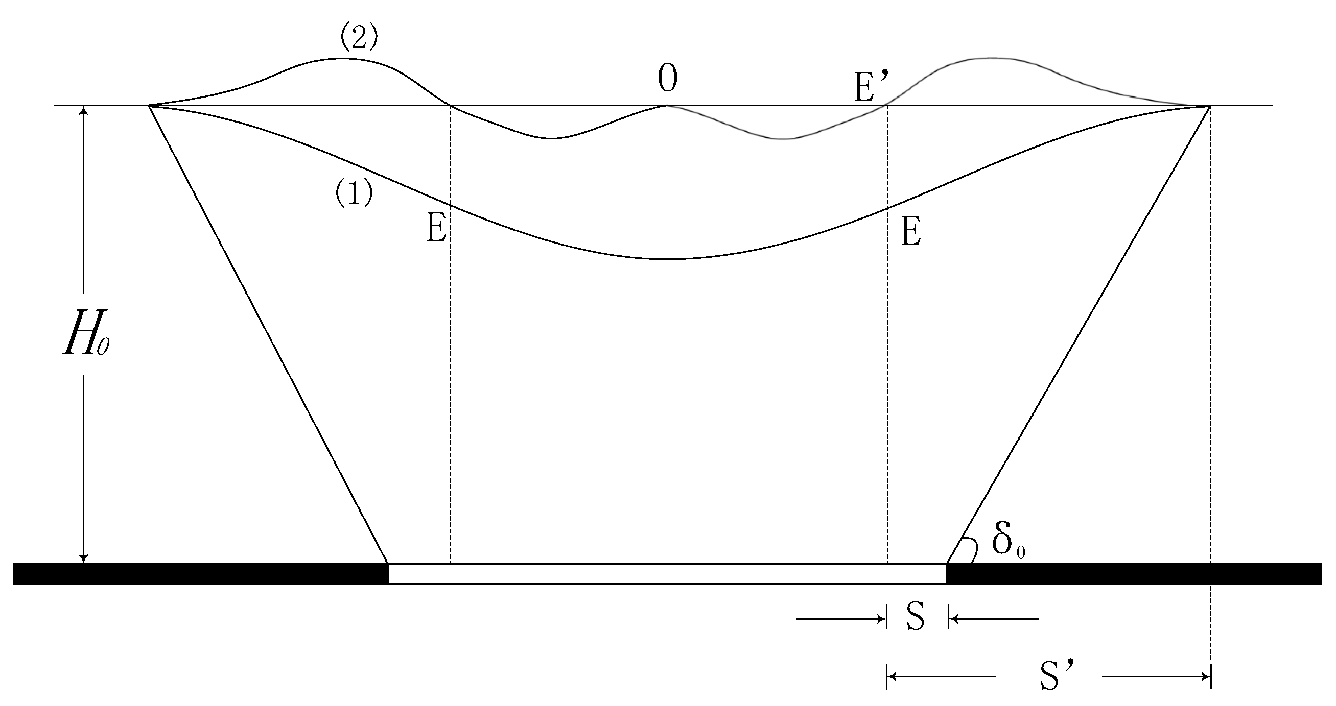
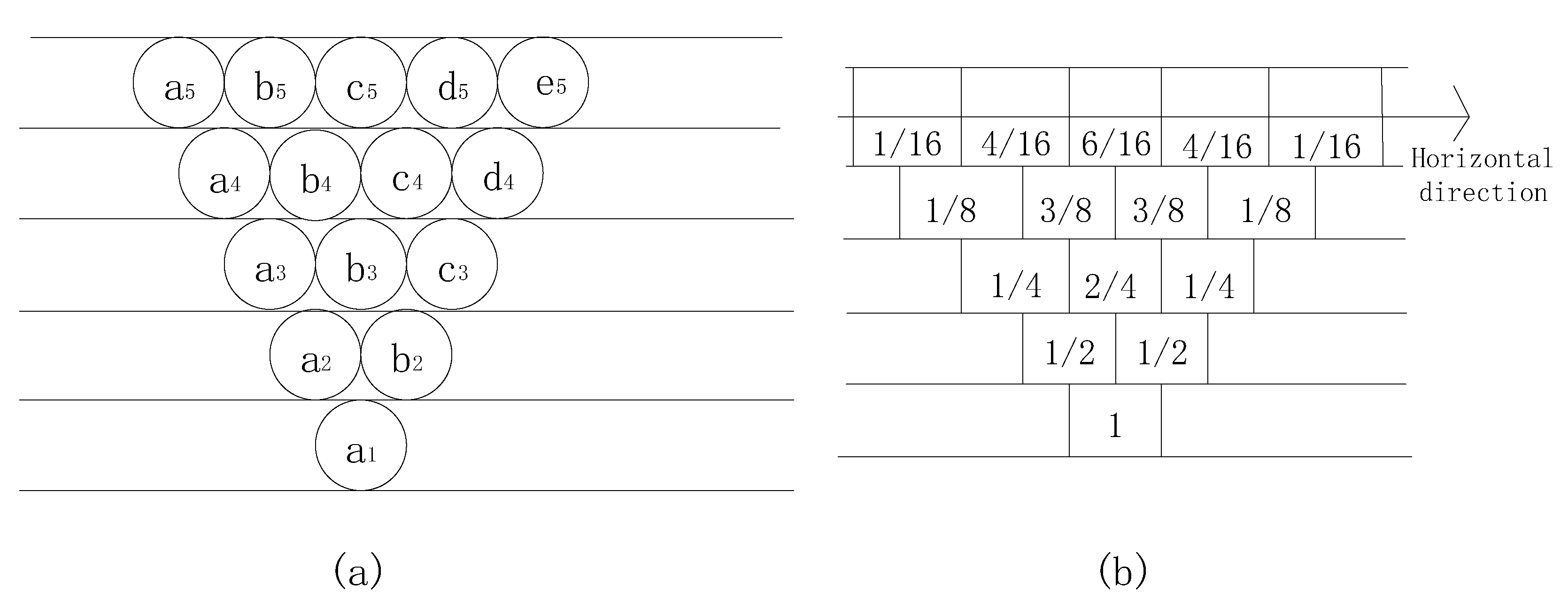
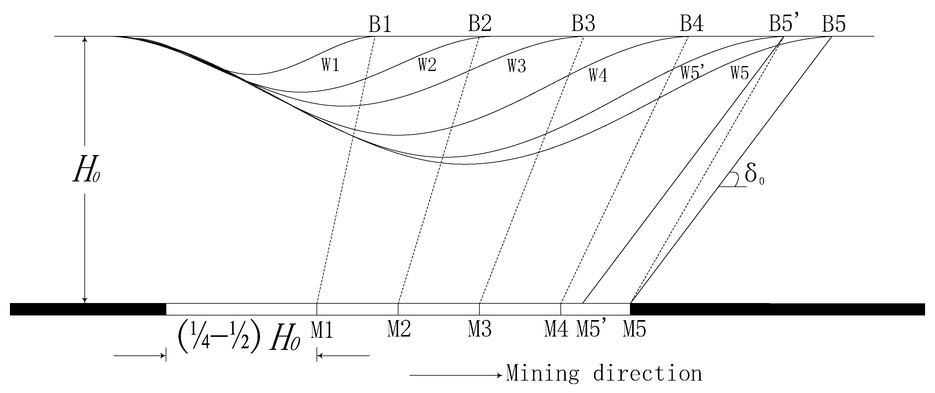
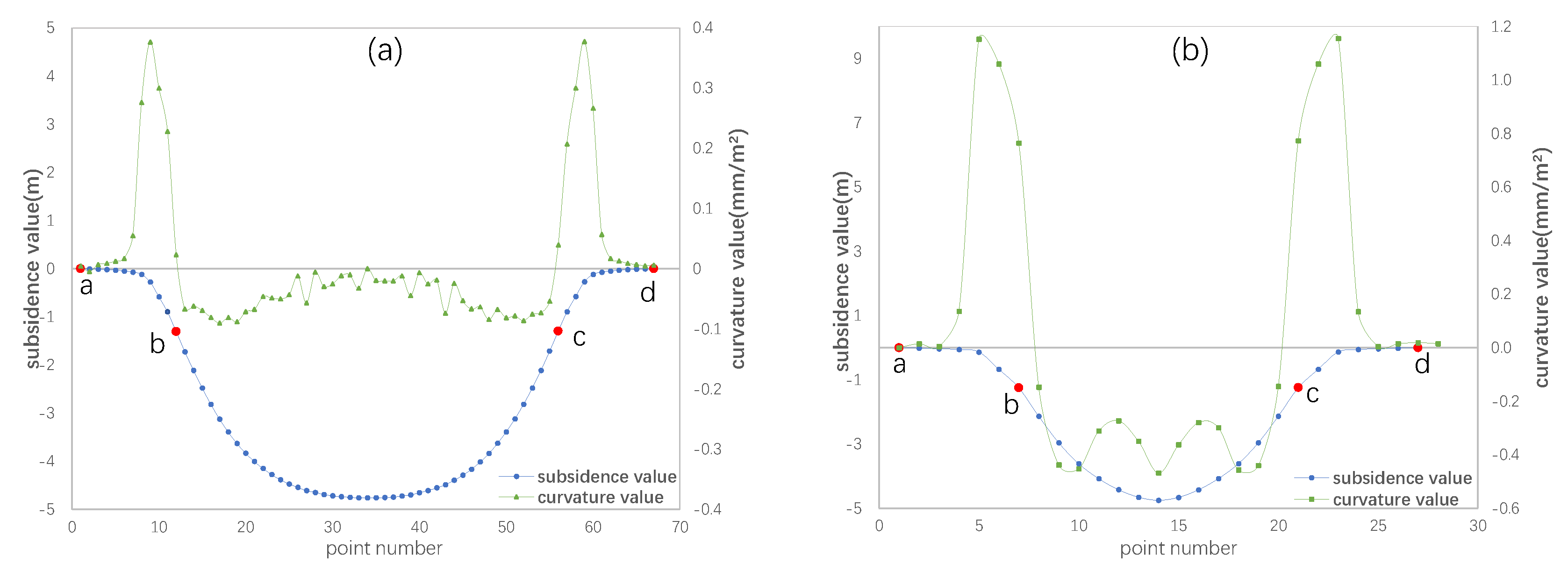
2.2. Feature Points of PIM

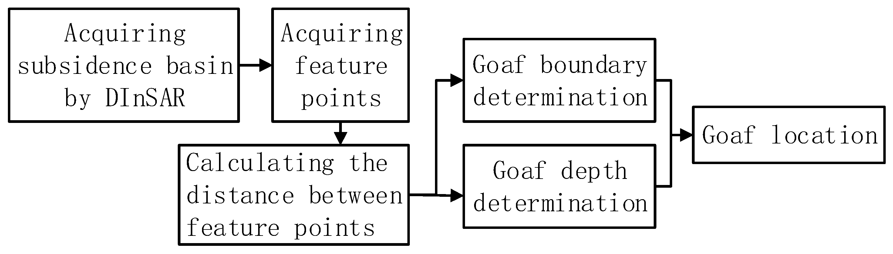
The PIM was first proposed by Polish scholars. It considers the movement of particulates, such as sand or tiny rock masses, as a random event, which makes the relationship between particulates irrelevant. The mining area can be divided into a number of differential units with the assumption that it is mined. The total impact of complete mining on the rock formation and the surface can be regarded as the integral of the small impact generated during the mining of the differential unit [25].

As shown in Figure 1a, when the ball (named $a_1$) on the first floor is taken away, one of the balls on the second floor ($a_2$ and $b_2$) will fall, so the probability of falling for each of the two balls is $1/2$. Then, one of the balls on the third floor will fall, and the falling probabilities for each of the three are $1/4$, $2/4$, and $1/4$, respectively (in Figure 1b). On this basis, the differential equation of the probability distribution function of the sinking event is obtained. For a clear expression, the plane, which is beyond the center of the subsidence basin and the vertical with horizontal, is appointed as the main section. The main section in the strike direction is called the strike main section, and the one in the dip section is called the dip main section. After assuming that the medium is infinitely small, in the main section, the surface subsidence profile equation of semi-infinite mining is

$$W(x)=\frac{W_{max}}{2}·[erf(\frac{\sqrt{\pi }}{r}·x)+1],$$

(2)

where $W(x)$ stands for the subsidence value at x; $W_{max}$ is the max value of the subsidence curve; r is the major influencing radius; $erf$ is the error function, and $erf=\frac{2}{\sqrt{\pi }}{\int }_0^x{e}^{-{\eta }^2}d\eta$. The location of $x=0$ is the coal mining boundary.

According to differential geometry, the second derivative of subsidence $W(x)$ is the curvature:

$$K(x)=\frac{d^{2}W(x)}{d{x}^2}/{[1+{(\frac{dW(x)}{d(x)})}^2]}^{\frac{3}{2}},$$

(3)

where $K(x)$ is the curvature at x. In the deformation basin, the value of ${(\frac{dW(x)}{d(x)})}^2$ is lower by more than three orders of magnitude. When it is neglected, the formula for calculating the curvature can be simplified to

$$K(x)=\frac{d^{2}W(x)}{d{x}^2}=2\pi \frac{W_{max}}{r^2}(-\frac{x}{r})e^{-\pi {(\frac{x}{r})}^2}.$$

(4)

According to Equation (4), when $x<0$, $K(x)>0$, the curve of $W(x)$ is upward convex; when $x>0$, $K(x)<0$, the curve of $W(x)$ is downward concave. Thus, the point at $x=0$ is the turning point between concave and convex geometries, and this is called the inflection point of the subsidence curve. That is to say, when the deformation of the overlying strata fully conforms to the law of a stochastic medium, the projection of the inflection point of the subsidence curve and the mining boundary point on the horizontal plane coincide. So, the inflection point can be used as a feature point to determine the goaf boundary.

The mining depth can be calculated by the inflection points and boundary points. As can be seen in Figure 2, $H_0$, ${\delta }_0$, $S^{\prime }$, and S satisfy the following trigonometric function relation:

$$tan({\delta }_0)=\frac{H_0}{S^{\prime }-S},$$

(5)

with ${\delta }_0$ and S obtained from [26]. $S^{\prime }$ can be obtained from the inflection point and the subsidence basin boundary point, so $H_0$ can be obtained by Equation (5). The four boundaries obtained by DInSAR can be used to calculate the mining depth.

2.3. Goaf Locating

Using the feature points, the boundaries and depth can be obtained. However, when calculating the boundaries, the actual situation is that the inflection point is located above the mining boundary and slightly deviates to the inside of the goaf. There are two reasons for the phenomenon: first, during mining activities, the roof caves in and forms a voussoir beam structure, which causes the roof near the mining boundary to bend stepwise or not fall, and there is a suspended roof distance; second, the fracture angle significantly affects the inflection point position. The actual surface subsidence and curvature curve caused by underground coal mining are shown in Figure 2.

In Figure 2, O is the basin center, $H_0$ is the mining depth, E is the inflection point of the subsidence curve, and $E^{\prime }$ is the zero point of the curvature curve. S is the deviation of the inflection point, that is, the distance between the projection of the inflection point on the coal seam plane and the mining boundary. $S^{\prime }$ is the projection of the distance from the boundary point of the basin to the zero point of the curvature curve $E^{\prime }$ on the horizontal plane. The parameter ${\delta }_0$ is the boundary angle in the main section, that is, the angle between the horizontal line and the line from the basin boundary point to the mining boundary point on the pillar side. As can be seen, the surface subsidence value is at its maximum above the center of the goaf and gradually decreases from the center of the basin to the edge, and it becomes zero at the basin boundary (the position at 10 mm subsidence is considered the boundary point during field measurements). The subsidence curve is symmetrical at the center. The curvature value is zero at the edge of the basin, it first increases and then decreases in the basin center’s direction and is zero again at the basin center. S is affected by many factors, such as the overlying rock properties and the existence of an adjacent goaf and geological structures. However, the deviation of the inflection point is usually considered a constant value in the same region in practical applications, because the geological conditions and strata attributes of the same area do not change much [26]. Obviously, this introduces some errors, but they are easily calculated.

After obtaining the subsidence basin by DInSAR, the inflection point E and deviation of the inflection point S can be used as feature points to determine the goaf boundary. For a flat coal seam, the two boundaries in the dip direction are symmetrical with respect to the center of the subsidence basin, so only one inflection point on either side of the dip direction is needed to obtain the two boundaries. The situation in the strike direction is more complicated. When monitoring the surface deformation by InSAR, the mining face is being mined, and because it takes time for the deformation to propagate in the overlying strata, the development of the surface deformation is delayed. This situation is described in Figure 3. In Figure 3, $(1/4\sim 1/2)H_0$ is the excavation distance of the working face when the ground surface begins to move. $M1\sim M5$ are the excavation positions of the working face from different periods, $W1\sim W5$ are the sink curves corresponding to $M1\sim M5$ when the ground surface movement is over, and $B1\sim B5$ are the boundary points of $W1\sim W5$. $W{5}^{\prime }$ is the sink curve when the excavation point has just reached $M5$ while the ground surface is still moving. $B{5}^{\prime }$ is the boundary point of $W{5}^{\prime }$. ${\delta }_0$ is the boundary angle in the main section, and $M{5}^{\prime }$ is the excavation point according to ${\delta }_0$. $M{5}^{\prime }$ is the calculation result for the mining boundary if the basin $W{5}^{\prime }$ is used, but it takes months for the basin to expand from $B{5}^{\prime }$ to $B5$. Therefore, in the locating process, according to geological conditions and prior experience, we move the characteristic points (inflection points and boundary points) to a certain distance in the mining direction to counteract the error caused by the surface deformation delay. When determining the depth, the excavating boundary may lead to a large error; the extraction size in the dip direction may not reach critical situation (the reason will be introduced in Section 5.3), so using the back basin boundary in the mining direction to calculate the mining depth will get better results. The sketch of the goaf locating can be represented by Figure 4.

3. Simulation Experiment

In order to verify the relationship between the characteristic points of the subsidence basin and the goaf position, the fast lagrangian analysis of continua (FLAC3D) was used to simulate mining activity, and the goaf position was then calculated according to the subsidence basin. FLAC3D adopts an explicit Lagrangian algorithm and a hybrid-discrete partition technique, which can simulate the plastic break and flow simulation parameters very accurately.

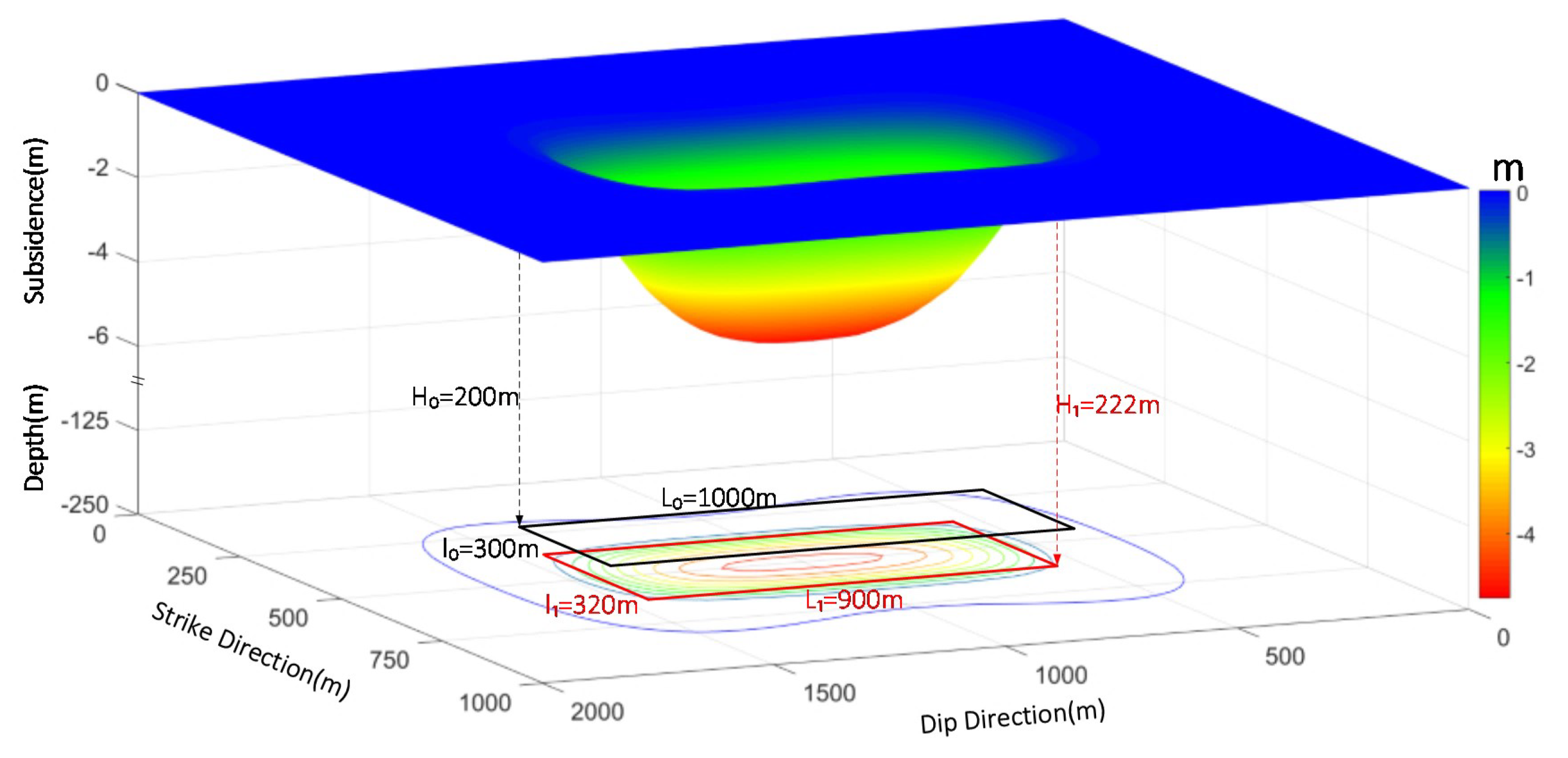
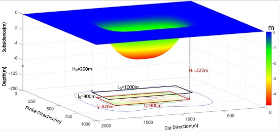
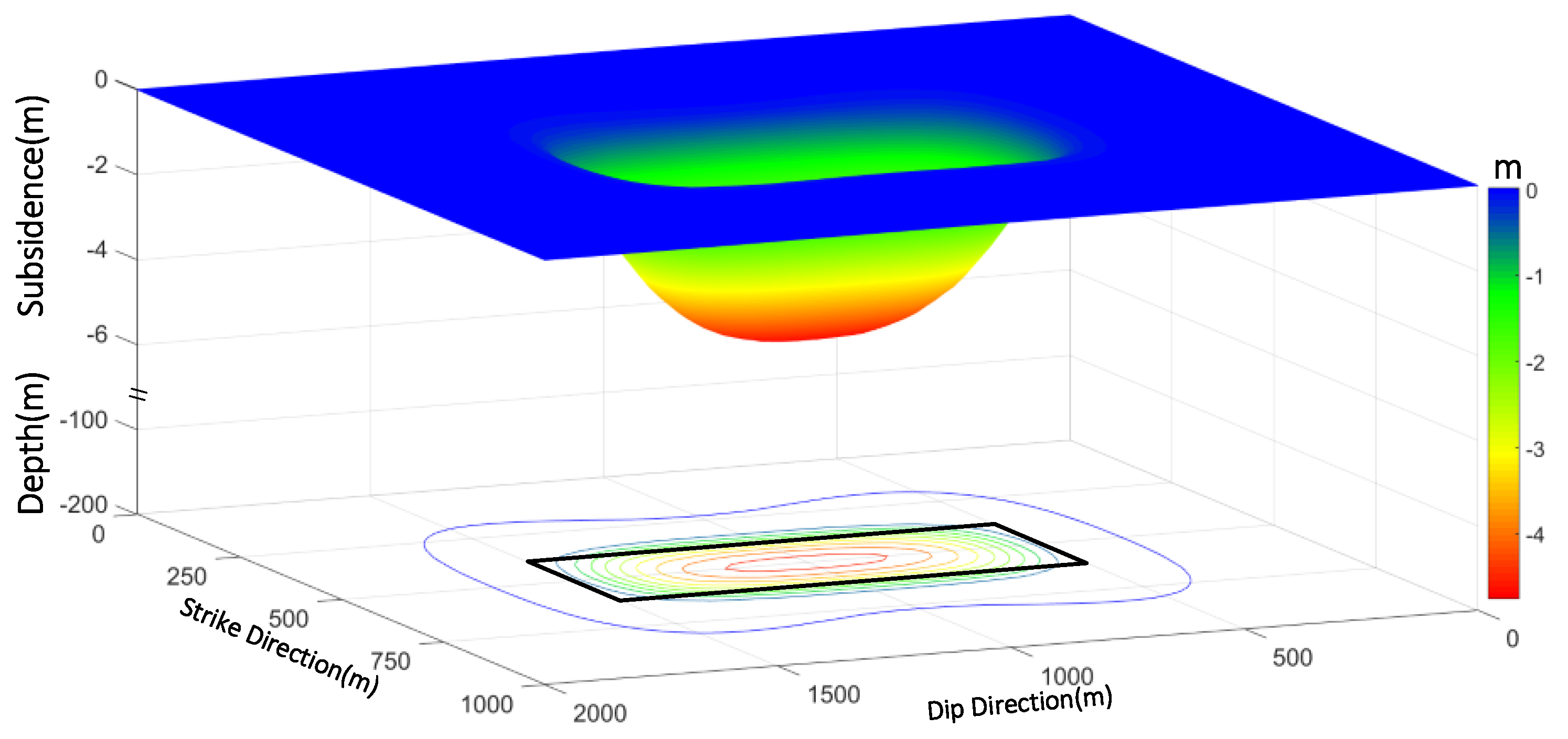
3.1. Numerical Simulation

In this simulation experiment, a horizontal working face was simulated with a mining depth of 200 m, a length of 1000 m, a width of 300 m, and a mining thickness of 7 m. The larger mining thickness and smaller mining depth ensured that the subsidence basin was fairly typical. The ratio of depth to thickness was close to 30, which ensured the continuity of the surface deformation. The horizontal resolution of the model block was 20 m × 20 m, which ensured the accuracy of the simulation while accounting for operational efficiency. The bottom, left, and right boundaries were constrained by horizontal displacement. The Mohr–Coulomb model was used to simulate the movement of the overlying rocks and surface subsidence. The Mohr–Coulomb model is a general model that is used to simulate mining activities [27]. It is a model applied to plastic materials and the calculation of deformation and stress according to the Mohr–Coulomb failure criterion (Equation (6)) and the maximum stress criterion.

$$\tau =\sigma ·tan(\mathsf{\Phi })+C,$$

(6)

where $\tau$ is the shear strength, $\sigma$ the normal stress, $\mathsf{\Phi }$ the angle of internal friction, and C the cohesion. Equation (6) was used to judge whether the principle stress caused shear failure, tensile failure, or no failure. Then, a different formula was used to calculate the plastic flow and new stresses. The loop computing ended until the maximum unbalanced force was lower than a threshold.

The mechanical parameters of the overlying strata were obtained from the histogram of a mining area in Pingdingshan, Henan, as shown in

Table 1. Mechanical parameters of the numerical simulation model.

Name of the Overlying Rock	Parameters of the Mohr–Coulomb Model
	Bulk	Shear	Cohesion	Tension	Friction
topsoil	4.3$\times {10}^7$	2.5$\times {10}^7$	4.1$\times {10}^4$	2.6$\times {10}^5$	1.8$\times {10}^1$
fine—sandstone1	2.5$\times {10}^9$	2.0$\times {10}^9$	1.9$\times {10}^6$	8.0$\times {10}^5$	3.0$\times {10}^1$
siltstone1	8.6$\times {10}^9$	6.6$\times {10}^9$	1.7$\times {10}^6$	4.4$\times {10}^5$	2.6$\times {10}^1$
siltstone2	8.6$\times {10}^9$	6.6$\times {10}^9$	1.7$\times {10}^6$	4.4$\times {10}^5$	2.6$\times {10}^1$
fine—sandstone2	2.5$\times {10}^9$	2.0$\times {10}^9$	1.9$\times {10}^6$	8.0$\times {10}^5$	3.0$\times {10}^1$
medium-sandstone1	3.5$\times {10}^9$	2.8$\times {10}^9$	1.9$\times {10}^6$	7.1$\times {10}^5$	3.3$\times {10}^1$
medium—sandstone2	3.5$\times {10}^9$	2.8$\times {10}^9$	1.9$\times {10}^6$	7.1$\times {10}^5$	3.3$\times {10}^1$
coal seam	8.3$\times {10}^9$	2.4$\times {10}^9$	3.2$\times {10}^6$	3.1$\times {10}^4$	2.7$\times {10}^1$
coal seam floor	8.6$\times {10}^9$	6.6$\times {10}^9$	1.4$\times {10}^6$	4.4$\times {10}^5$	2.6$\times {10}^1$

.

The mining activity and the surface deformation were simulated, and the subsidence basin was obtained when the ground surface was stable (where the unbalanced force is less than ${10}^{-5}$ of the maximum unbalanced force).

As can be seen in Figure 5, the maximum subsidence point was in the center of the basin, and the maximum subsidence value was 4.76 m. The tilt and curvature were obtained by taking the first-order and two-order derivative of the subsidence basin (shown in Figure 6). To facilitate the display, the acquired tilt and curvature were processed by mirroring. The value represented by the tilting and curvature map was opposite to the true curvature and the tilt value.

As can be seen in Figure 6, the wave crest and wave trough were opposite to the main section in the dip direction and the strike direction in graphs (1) and (2), respectively. In graph (1), there is a distance between the edges of the hump and the pit, while there is nearly no such distance in graph (2), which indicates that the mining degree in the strike direction is larger than that in the dip direction. In graphs (3) and (4), the curvature was negative at the edge and positive in the center. For the positive areas, the curvature value was large at the edge and small in the center in graph (3); this is contrary to that in graph (4), which indicates that the mining degree was full in the strike direction and subcritical in the dip direction. In order to more clearly show the variation in the subsidence and curvature curves, we obtained the subsidence curve and the curvature curve on the strike main section and the dip main section. The result is shown in Figure 7. In Figure 7, graph (a) shows that the bottom of the subsidence curve was gentle. The value of the curvature curve decreased after first increasing, and it then continued to increase until it was zero from the edge to the center and zero at the inflection point, indicating that the mining degree in the strike direction was full. In graph (b), the bottom of the subsidence curve is sharp. The value of the curvature curve decreased after increasing; it then fluctuated below the axis and was zero at the inflection point, indicating that the mining degree was subcritical in the dip direction.

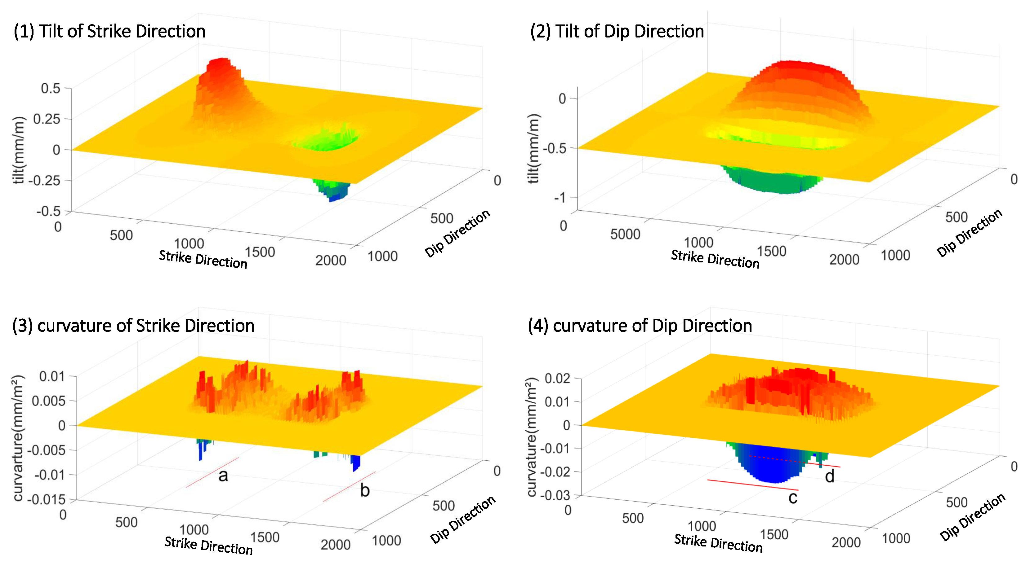
3.2. Simulated Goaf Locating

Equation (3) shows that the inflection point was close to the goaf boundary after projection on the horizontal plane. If the red lines (a, b, c, d in Figure 6) are moved by the distance of the deviation of the inflection point toward the side of the coal pillar, they become the goaf boundary. Therefore, according to Equation (4) and the position of the inflection point and boundary point in the main section, the mining depth can be determined. Because the simulation data were ideal (as shown in Figure 5), there was no need to fit the subsidence curve.

According to [26], the boundary angle ${\delta }_0$ is ${51}^{\circ }$, and the deviation of the inflection point S was 20 m. Because the basin was stable, there was no need to consider the delay distance. The result is shown in Figure 8.

As can be seen in Figure 8, the length of the calculated goaf was smaller than the real one, but the calculated width and depth are larger. According to Equation (5), the depth is directly proportional to the distance from the mining boundary to the basin boundary: thus, the larger the length, the smaller the depth. This conclusion agrees with the experimental result.

3.3. Accuracy Evaluation

In order to accurately evaluate the error of this method, the calculated goaf location was compared with the position of the goaf in the simulation model. The error of the simulation experiment is shown in

Table 2. Comparison of locating results and the simulated model.

	Length	Width	Depth
Real value	1000 m	300 m	200 m
Calculated value	900 m	320 m	222 m
Absolute boundary error	$-50$ m	10 m	22 m
Relative boundary error	$-5.00$%	3.30%	11.00%

. Table 2 shows that the length of the calculated goaf was smaller than the real length, and the relative error was 5.00%. Because there was no need to consider the delay distance and the mining degree in the strike direction was full, the error of the goaf boundary in the strike direction can be assumed to be mainly caused by the deviation of the inflection point and simulated block resolution. The crushing and deformation during mining caused the plasticity of the overlying strata to decrease, which led to a decrease in the length of the voussoir beam structure and a slight change in the deformation propagating in the overlying strata. The empirical value of the deviation inflection point was obtained with the measured data from monitoring the mining subsidence deformation, so the change in the overlying strata properties were reflected in the empirical value. However, once the mechanical parameters of the overlying strata were set in the simulation experiment, it was difficult to modify them during the simulation calculation process, and this resulted in a larger inflection point deviation. Since the inflection point deviation was not reduced properly in the goaf boundary calculation process, the calculated strike boundary was shifted to the basin center because of the parameter change. The resolution of the ground observation points was 20 m, and the inflection point can only be located at one point and cannot be between two points. So, the maximum error caused by the resolution could have reached 10 m, and the direction was uncertain. The mining degree in the dip direction was subcritical, which causes the inflection point to shift away from the basin center, and this error was in the opposite direction of the parameter change. Compared with the real goaf boundary, the calculated boundary shifted away from the basin center, indicating that the error caused by subcritical mining was greater than that caused by the parameter change. The mining depth was calculated by the boundary behind the mining direction and inflection point, so it was not affected by subcritical mining and delay distance. The boundary angle, inflection point deviation, strike boundary position, and observation point resolution were the main error sources for calculating the goaf depth. Similar to the error source of the inflection point deviation, the property of the overlying strata changed with deformation, but the mechanical parameters in the numerical simulation model were always constant; this led to a smaller boundary angle in the simulation experiment than the empirical value used in the real experiment, resulting in a smaller calculated value of the mining depth. In general, the combined influence of the boundary angle, inflection point deviation, and basin observation point resolution results in a calculated mining depth that is larger than the actual value. Compared with the real data experiment, the simulation experiment was simple and not affected by complex geological conditions. The error sources were all model errors. Therefore, the average model errors of the proposed method were considered to be 4.15% and 11.00% when calculating the boundary and depth of the goaf, respectively.

4. Real Data Experiment

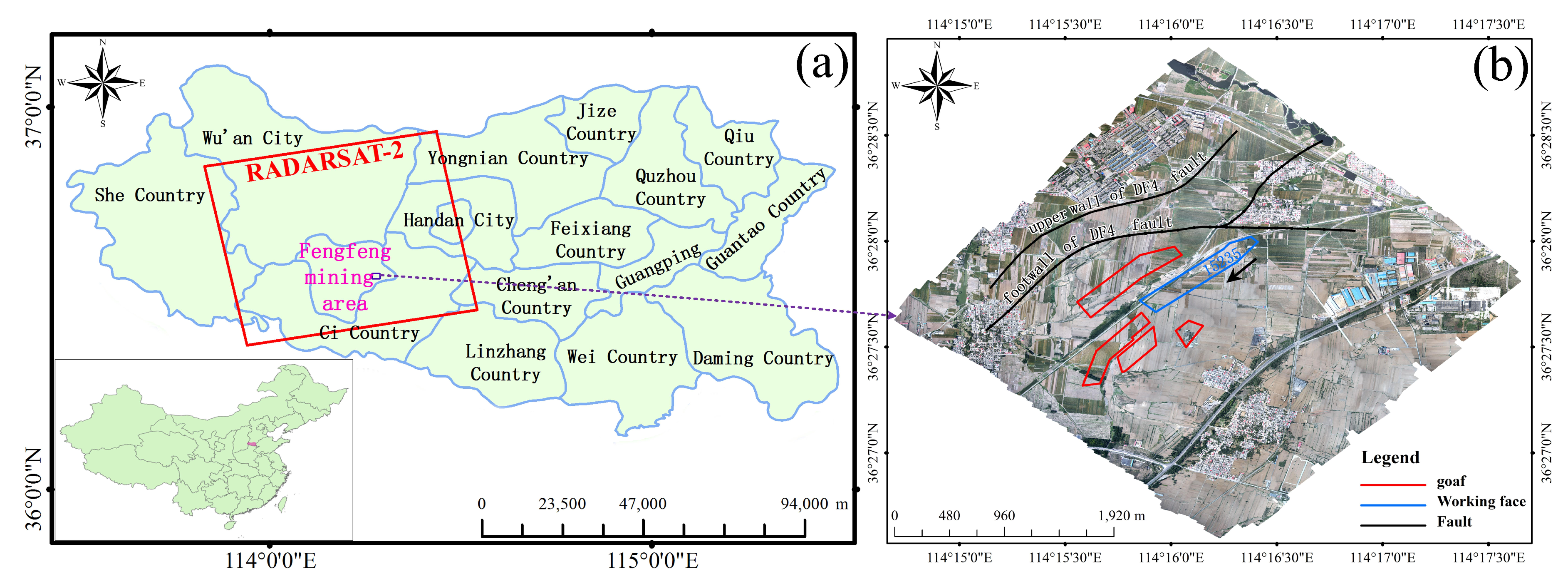
4.1. Study Area

The 15235 working face of the Jiulong mining area is located in Fengfeng coalfield, Hebei Province, China. It has a length of 935 m in the strike direction, a length of 142 m in the dip direction, an average coal mining thickness of 4.5 m, and an average mining depth of 740 m. The inclination of the working face is ${13}^{\circ }$. When the inclination of the coal seam is less than ${15}^{\circ }$, the surface deformation caused by mining can be regarded as being the same as that caused by horizontal coal seam mining [20]. As can be seen in Figure 9, there is a large fault and some old goafs located in the northwest and west, respectively, which may affect the location accuracy.

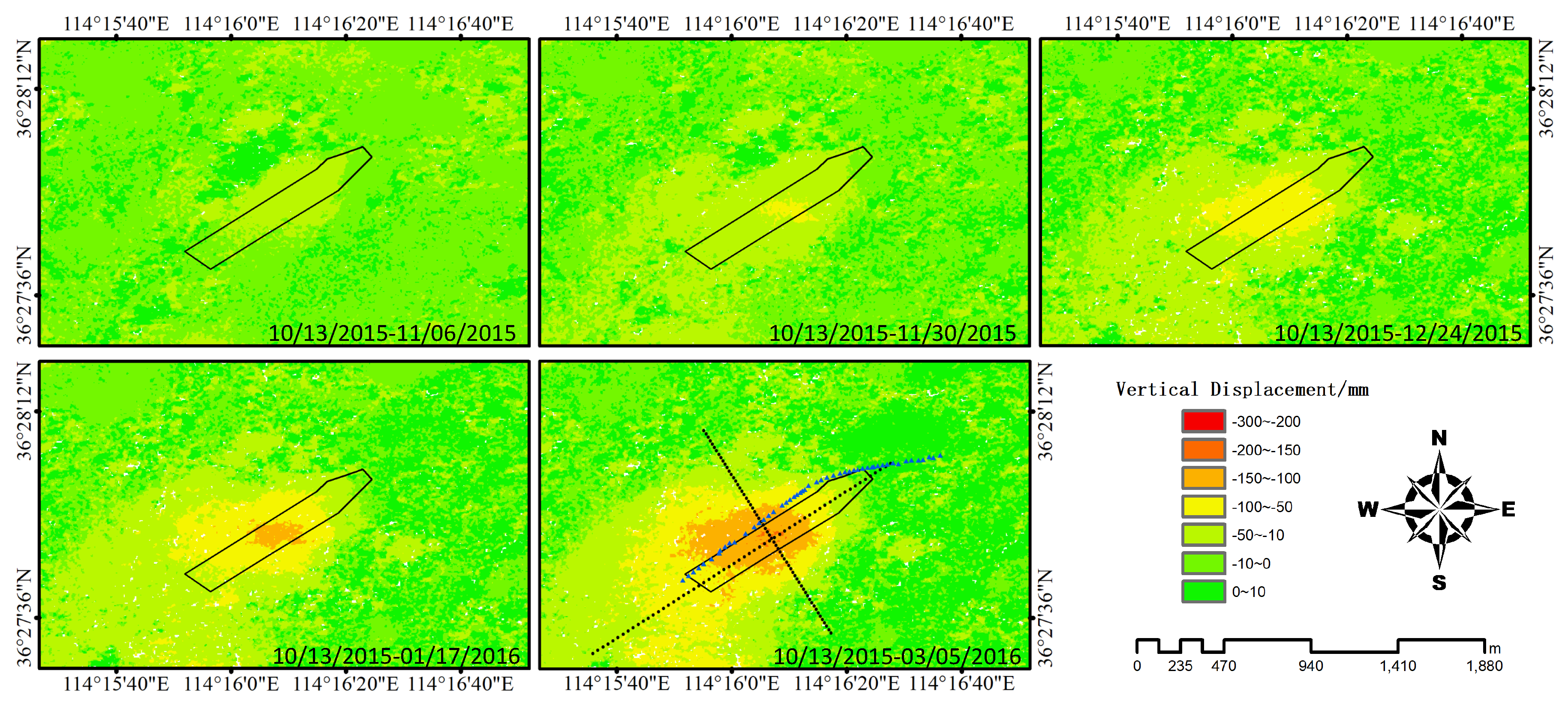
4.2. DInSAR Data Processing

Six images of RADARSAT-2, collected from 13th October 2015 to 5th March 2016, were used to obtain the subsidence basin using the multi-look fine mode. Five interferograms were formed with the parameters shown in

Table 3. Parameters of interferogram pairs.

Interferograms Pairs	Spatial Baseline	Time Baseline
20151013–20151106	47.1835 m	24 d
20151106–20151130	3.8988 m	24 d
20151130–20151224	13.3323 m	24 d
20151224–20160117	−43.7693 m	24 d
20160117–20160305	−37.7825 m	48 d

. The coverage of the images is shown in Figure 9 with the red rectangle. SRTM data with a resolution of 3 seconds (90 m) were used as an external DEM to remove the terrain phase from the interferograms. The study area was small, so the atmospheric errors can be ignored [28]. The orbit error can also be ignored because of the highly precise measurement and control of the attitude of the RADARSAT-2 satellite [29]. Adaptive filtering and low-pass filtering were used to reduce noise effects.

The interference results were used to calculate the surface LOS deformation. The time series surface subsidence can be obtained by projecting the LOS deformation in the vertical direction and stacking the images. If we assume that there is no horizontal movement, then the vertical deformation equals the LOS deformation divided by the cosine of the incident angle. The influence of this assumption is analyzed in Section 5.1.

As can be seen from Figure 10, the subsidence basin continued to expand, and the maximum subsidence value increased continuously and developed toward the southwest. Perhaps as a result of the influence of the surrounding geological conditions and the old goaf, the edge of the subsidence basin developed toward the northwest and southwest. This was inconsistent with the development direction of the subsidence basin center and will affect the final location results.

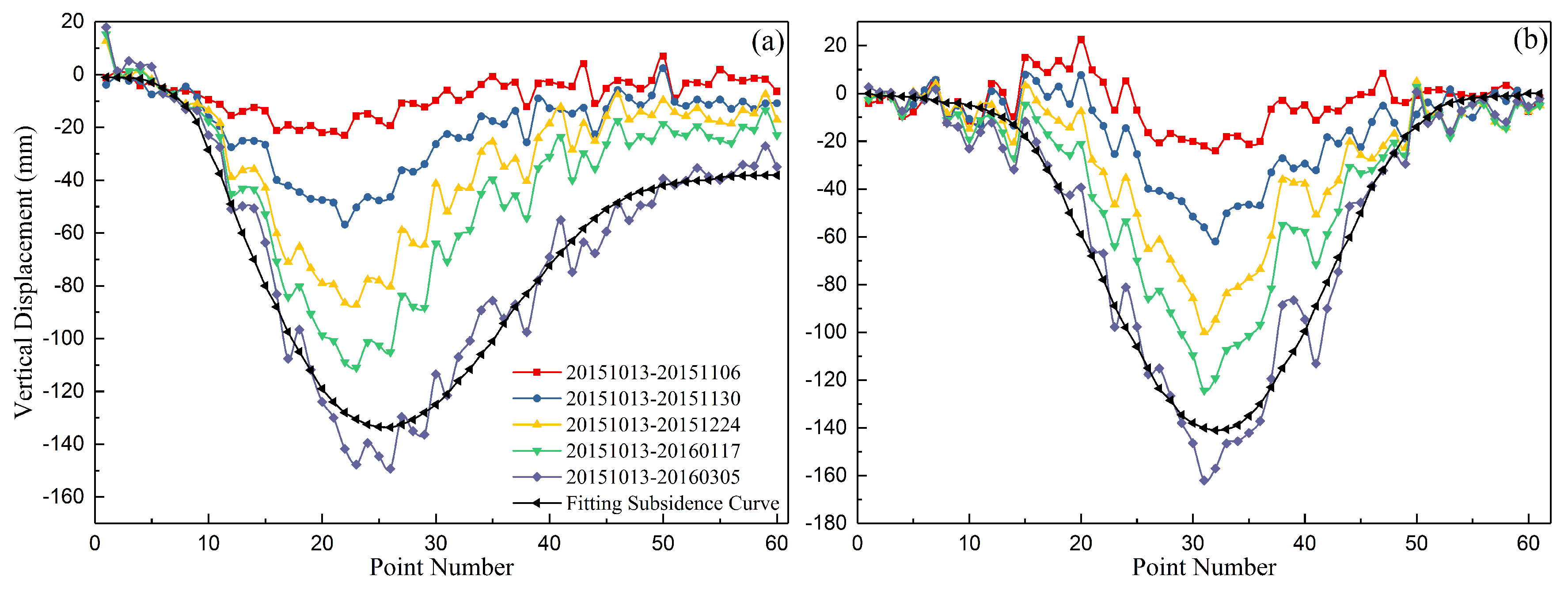
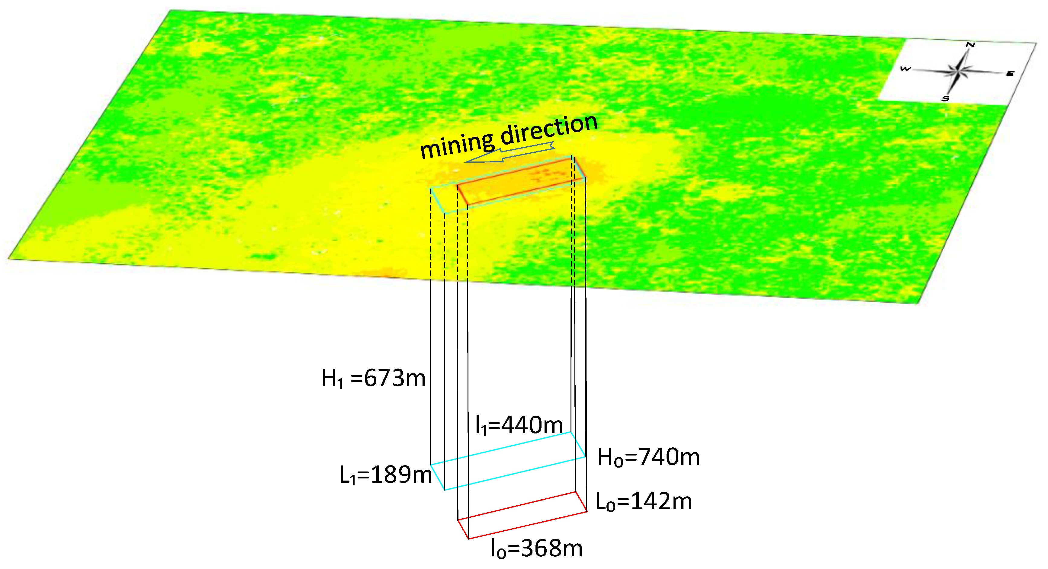
4.3. Goaf Location Process and Result

According to the development trend of the subsidence basin center in Figure 10, the mining strike azimuth was about ${236}^{\circ }$. Two observing lines were made that were perpendicular to each other along the strike and dip directions and passed through the subsidence center. Sixty sampling points (black dots in Figure 10) were set at equal distances on each observing line. The subsidence value of the sampling point position was extracted from Figure 10 to obtain the subsidence curves in the strike and dip directions.

In Figure 11, it can be seen that the subsidence value at each sampling point increased over time, and the closer the point was to the subsidence basin center, the greater the subsidence value. The maximum subsidence value was 148 mm. Some points on the subsidence curves in the strike and dip directions showed positive values in the first three observation periods, indicating that there was uplift on the surface of the corresponding sampling points. The subsidence curves fluctuate in the strike and dip directions. The five subsidence curves in each graph fluctuate with the same trend, indicating that the cause of the fluctuation was the uneven surface subsidence, not the DInSAR observation error. In order to display the law of the subsidence curve more clearly and determine the inflection point more accurately, the subsidence curve was fitted. The end of the fitting curve in the strike direction did not tend to zero, which coincides with the subsidence graph in Figure 10. It further confirms that the edge of the subsidence basin was affected by geological structures or the goaf, which led to changes in its distribution. Therefore, when locating the boundary in the dip direction, the inflection point in the southeast was calculated first to determine the southeast boundary in the dip direction, and then the northwest boundary in the dip direction could be determined by the symmetry of the subsidence basin to avoid the error caused by the edge shifting of the subsidence basin. In this experiment, the proposed method was used to locate the goaf. First, the planimetric position of the working face 15,235 was determined according to the inflection points. With reference to the geological conditions of the Fengfeng mining area and other working faces, the deviation of the inflection point was set to 20 m, the boundary angle was set to ${57}^{\circ }$, and the delay distance was set to 100 m. If the basin boundaries in the dip direction were used to calculate the mining depth, the result can be affected by the subcritical mining degree. If the southeast boundary was used to calculate the mining depth, the result can be affected by the subsidence delay. Therefore, the mining depth was calculated by the northeast boundary in the strike direction, and the final location result was obtained (Figure 12).

It can be seen in Figure 12 that the calculated northeast mining boundary in the strike direction and the mining boundary in the dip direction were close to the real mining boundaries. The calculated southwest mining boundary was far from the real mining boundary, and this was because the geological structure and old goaf affect the subsidence basin. The calculated northeast mining boundary in the strike direction was located inside the real mining boundary, while the calculated mining boundary in the dip direction is located outside the real mining boundary; these findings were consistent with the simulation experiment, indicating that insufficient mining causes the calculated mining boundary to shift outward.

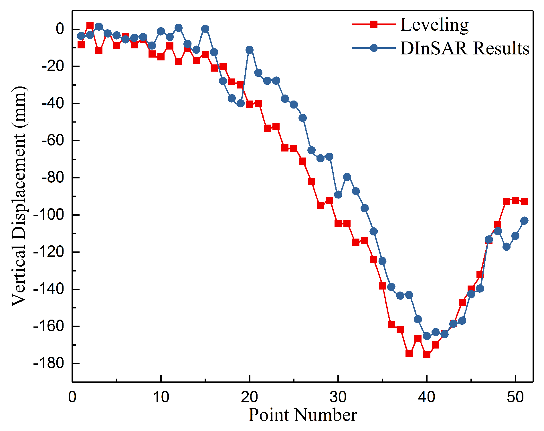
4.4. Precision Analysis

In order to evaluate the accuracy of this real data experiment, we calculated the absolute and relative error between the calculated mining boundary and the real mining boundary shown in

Table 4. Errors of calculated results.

	Northwest	Southeast	Southwest	Northeast	Depth	Average Value
Absolute error (m)	22.58	23.45	74.58	4.52	67.12	38.45
Relative error	15.90%	16.51%	20.25%	1.23%	9.07%	12.59%

(the relative error is the ratio of the absolute error to the mining length in the strike or dip direction).

The absolute errors of the southwest boundary and the boundaries in the dip direction were about 75 and 23 m, respectively, which were larger than the absolute errors of 50 m and 10 m in the simulation experiment. It was shown that the simulation experiment’s neglected factors, such as DInSAR observation error and geological structure, had a great influence on the calculated results. Although the northwest boundary was obtained by symmetry, its error was different from that of the southeast boundary because the center of the subsidence basin was not located in the center of the working face. The error of the calculated mining depth was 9.07%, which was close to the error of 11.00% in the simulated experiment. Overall, the average relative error was 12.59%, and the average absolute error was about 38 m. The average error of the planar positioning was about 31 m. This accuracy was sufficient for engineering applications that require the positioning of the goaf (illegal mining location, goaf records, etc.). With an error of 67 m in depth determination and the geological data of the study area, we can determine the coal seam where the mining activity was located. Therefore, the accuracy of the method in this paper is acceptable.

5. Discussion

5.1. Influence of DInSAR on the Location Result

Observed errors inevitably occur when using DInSAR to obtain surface deformation. In addition, the LOS deformation monitored by DInSAR is directly transformed into vertical deformation without considering the horizontal movement in the real data experiment. In order to verify the accuracy of the DInSAR monitoring results, the leveling data above the working face were used. The blue triangles represent the positions of the 51 leveling points arranged from northeast to southwest in Figure 10. The dates on which the first and last leveling data were measured were 10th October 2015 and 4th March 2016, respectively, which are similar to the acquisition times of the first and last SAR images. If the subsidence rate is regarded as a constant value, a time difference of two days will lead to an error of only 2.3%, so the influence of time inconsistency is very small. The comparison is shown in Figure 13.

It can be seen from Figure 13 that the DInSAR monitoring result coincides with the leveling data. The maximum deviation is 31.5 mm, located at point 38; the minimum deviation is less than 0.1 mm, located at point 4; the average error is 8.5 mm; the root-mean-square error is 15.7 mm. With the horizontal movement ignored, the LOS deformation detected by DInSAR is considered to consist only of the component of the vertical surface deformation in the LOS direction. In fact, the components of the horizontal surface deformation in the LOS direction are also the components of the LOS deformation. Taking a point in the dip main section as an example (Figure 14), the LOS deformation obtained by DInSAR is composed of the component of vertical deformation in the LOS direction and the component of the horizontal deformation in the LOS direction (the blue arrow in Figure 14). In this example, the two components have the same direction. The LOS deformation is a fixed value that is obtained by DInSAR. When horizontal deformation is neglected, the vertical deformation will increase and become larger than the true value so that its component will be the same as the LOS deformation. The converse is also true: that is to say, if the component of the horizontal movement in the LOS direction is the same as the direction of the satellite incident angle, ignoring the horizontal movement will lead to the vertical deformation being larger than the true value; if the component of the horizontal movement in the LOS direction is opposite to the direction of the satellite incident angle, ignoring the horizontal movement will lead to the vertical deformation being smaller than the true value. The SAR data used in this experiment were orbit-lifting. The heading angle of the satellite is about $-{10}^{\circ }$, and the azimuth angle of the working face is about ${236}^{\circ }$. The horizontal movement caused by mining the working face is toward the center of the subsidence basin in both the strike and dip directions. Therefore, the subsidence value is larger in the western part of the subsidence basin, while, in the east part of subsidence basin, the subsidence value is smaller. In Figure 13, points 1–40 are located in the eastern part of the subsidence basin, and most of the DInSAR data are smaller than the leveling data. Points 40–51 are located in the western part of the subsidence basin, and most of the DInSAR data are larger than the leveling data, which is consistent with the above conclusions. On the whole, the subsidence curve migrates to the southwest after neglecting the horizontal movement, resulting in the calculated mining boundary shifting toward the southwest. With respect to the real data experiment, the calculated northeast boundary is located inside the real boundary, which also confirms this conclusion. Therefore, with multi-platform InSAR data to calculate the three-dimension deformation, the precision of InSAR measurements will increase.

5.2. Influence of Geological Structure on the Location Result

It can be seen from Figure 10 and Figure 12 that although the position of the maximum subsidence point of the surface subsidence basin is still inside the working face, the edge of the basin shifts toward the northwest and southwest. As can be seen in Figure 9, the position of the faults and old goafs are consistent with the basin’s shifting direction, so the reason for the basin shifting may be that the mining activity of 15235 activates the overlying strata of faults and old goafs, which causes the subsidence beyond the surface. The shifting of the basin edge results in the migration of inflection points and boundary points. If the inflection point on the northwest side is used to locate the mining boundary, the absolute error is 123.95 m, and the relative error is 87.29%. This indicates that it is reasonable to directly use symmetry to locate the mining boundary.

5.3. Influence of Subcritical Extraction on the Location Result

According to experience from mining subsidence studies, the relationship between the mining degree and the ratio of mining size to depth is as follows [20]: when $D_1/H_0$, $D_3/H_0<1.2\sim 1.4$, the mining degree is subcritical; when $D_1/H_0$, $D_3/H_0=1.2\sim 1.4$, the mining degree is full; when $D_1/H_0$, $D_3/H_0>1.2\sim 1.4$, the mining degree is super full, where $D_1$ and $D_3$ are the lengths in the dip and strike direction, respectively, and $H_0$ is the mining depth. The range $1.2\sim 1.4$ is the experience value related to the properties of the overlying rock. The ratio of the length in the dip and strike directions to the mining depth of 15235 is 0.2 and 1.09, respectively, which means that the mining degree of 15235 is close to full in the strike direction and is subcritical in the dip direction. With the increase in mining degree, the inflection point moves from the outside to the inside of the mining boundary [20]. Therefore, in the simulation experiment and the real data experiment, the mining degrees in the dip direction are subcritical, so the calculated mining boundary is outside of the real mining boundary in the dip direction.

6. Conclusions

The proposed method uses the feature points of the basin monitored by DInSAR to locate the goaf. The method has the advantages of having a low economic cost and a high degree of automation compared with the traditional geophysical approaches. Although the PIM is taken as the theoretical basis, this method does not depend on a complex model algorithm or the model parameters of the probability integral method (such as subsidence coefficient, tangent of the main influence angle, etc.), and fewer parameters mean less uncertainty and better prospects for engineering applications. A simulation experiment and real data experiment were carried out to verify the reliability and accuracy of the proposed approach. The average relative errors of the simulation experiment and real data experiment are 6.43% and 12.59%. Because the basin is directly calculated in the simulated experiment, the errors come from the model. The relative error of the real data experiment is twice that of the simulated experiment; thus, the errors of the model and of the rest of the factors have the same order of magnitude. The experiments prove that the results of DInSAR monitoring can be used to locate the goaf because the DInSAR precision is good enough to accurately obtain the shape of the basin.

In this method, the accuracy of the shape and the feature points of the basin is more important than the deformation accuracy obtained by DInSAR monitoring. The mining degree affects the relative position of the inflection points and the goaf boundaries. The lower the mining degree, the farther the inflection points from the boundaries, so a subcritical extraction leads to the calculated goaf width being smaller than the actual value. Ignoring the horizontal movement causes the migration of the basin, and then the whole calculated goaf has an offset. Therefore, a high-precision observation method helps to improve the accuracy of this method. In our future work, we will focus on the influence of coal seam inclination, geological structure, and subcritical mining on the location results.

References

1. Liu, M.; Zeng, Y. Study on Geological Hazards Due to Mining Subsidence and Their Countermeasures in Mining Area. Jiangsu Environ. Sci. Technol. 2005, 18, 29–32. [Google Scholar]
2. Yu, X.Y.; Qiu, Y.X. Analysis of subsidence status formation mechanisms in shallow mining seam of ravine cutting area. J. Xi’an Univ. Sci. Technol. 2012, 32, 269–274. [Google Scholar]
3. Guo, W.-B.; Deng, K.-Z.; Zou, Y.-F. Research Progress and Prospect of the Control Technology for Surface and Overlying Strata Subsidence. China Saf. Sci. J. 2005, 15, 6–10. [Google Scholar]
4. Zhou, S.-D.; Wang, X.-X.; Li, T.-J. Geological Environmental Problems Induced by Coalfield Exploition and Control Countermeasures. Res. Soil Water Conserv. 2007, 14, 351–354. [Google Scholar]
5. Jia, Z.; Suo, K.; Song, Z.; Zhang, G. Goal Mine Detection with Transient Electromagnetic Method and Magnetic Method. Chem. Eng. Trans. 2018, 66, 1249–1254. [Google Scholar]
6. Fan, H.; Deng, K.; Ju, C.; Zhu, C.; Xue, J. Land subsidence monitoring by D-InSAR technique. Min. Sci. Technol. (China) 2011, 21, 869–872. [Google Scholar] [CrossRef]
7. Fan, H.; Gao, X.; Yang, J.; Deng, K.; Yu, Y. Monitoring mining subsidence using a combination of phase-stacking and offset-tracking methods. Remote Sens. 2015, 7, 9166–9183. [Google Scholar] [CrossRef]
8. Yang, Z.F.; Li, Z.; Zhu, J.J.; Hu, J.; Wang, Y.J.; Chen, G.L. InSAR-Based Model Parameter Estimation of Probability Integral Method and Its Application for Predicting Mining-Induced Horizontal and Vertical Displacements. IEEE Trans. Geosci. Remote Sens. 2016, 54, 4818–4832. [Google Scholar] [CrossRef]
9. Zhu, Y.-F.; Yu, J.; Wu, J.-Q.; Wu, S.-L.; Li, X.-Q.; Zhang, J.-F.; Luo, Y.; Su, Y.-M. Application comparison of D-InSAR and PS-InSAR techniques in Suzhou land subsidence monitoring. J. Geol. 2010, 34, 289–294. [Google Scholar]
10. Solari, L.; Ciampalini, A.; Raspini, F.; Bianchini, S.; Zinno, I.; Bonano, M.; Manunta, M.; Moretti, S.; Casagli, N. Combined use of C-and X-Band SAR data for subsidence monitoring in an urban area. Geosciences 2017, 7, 21. [Google Scholar] [CrossRef]
11. Solari, L.; Del Soldato, M.; Bianchini, S.; Ciampalini, A.; Ezquerro, P.; Montalti, R.; Raspini, F.; Moretti, S. From ERS 1/2 to Sentinel-1: Subsidence monitoring in Italy in the last two decades. Front. Earth Sci. 2018, 6, 149. [Google Scholar] [CrossRef]
12. Han, Y.-F.; Song, X.-G.; Shan, X.-J.; Qu, C.-Y.; Wang, C.-S.; Guo, L.-M.; Zhang, G.-F.; Liu, Y.-H. Deformation monitoring of Changbaishan Tianchi volcano using D-InSAR technique and error analysis. Chin. J. Geophys. 2010, 53, 1571–1579. [Google Scholar]
13. Di Traglia, F.; Nolesini, T.; Solari, L.; Ciampalini, A.; Frodella, W.; Steri, D.; Allotta, B.; Rindi, A.; Marini, L.; Monni, N.; et al. Lava delta deformation as a proxy for submarine slope instability. Earth Planet. Sci. Lett. 2018, 488, 46–58. [Google Scholar] [CrossRef]
14. Goldstein, R.M.; Engelhardt, H.; Kamb, B.; Frolich, R.M. Satellite radar interferometry for monitoring ice sheet motion: application to an Antarctic ice stream. Science 1993, 262, 1525–1530. [Google Scholar] [CrossRef] [PubMed]
15. Li, X.X. An Illegal Mining Detection Method Based on D-InSAR. Master’s Thesis, China University of Mining and Technology, Xuzhou, China, 2012. [Google Scholar]
16. Hu, Z.; Ge, L.; Li, X.; Zhang, K.; Zhang, L. An underground-mining detection system based on DInSAR. IEEE Trans. Geosci. Remote Sens. 2013, 51, 615–625. [Google Scholar] [CrossRef]
17. Xia, Y.; Wang, Y.; Du, S.; Liu, X.; Zhou, H. Integration of D-InSAR and GIS technology for identifying illegal underground mining in Yangquan District, Shanxi Province, China. Environ. Earth Sci. 2018, 77, 319. [Google Scholar] [CrossRef]
18. Yang, Z.; Li, Z.; Zhu, J.; Yi, H.; Feng, G.; Hu, J.; Wu, L.; Preusse, A.; Wang, Y.; Papst, M. Locating and defining underground goaf caused by coal mining from space-borne SAR interferometry. ISPRS J. Photogramm. Remote Sens. 2018, 135, 112–126. [Google Scholar] [CrossRef]
19. Peng, S.S.; Ma, W.; Zhong, W. Surface Subsidence Engineering; Society for Mining, Metallurgy, and Exploration Littleton: Englewood, CO, USA, 2005. [Google Scholar]
20. Deng, K.Z.; Tan, Z.X.; Jiang, Y. Subject of Deformation Monitoring and Subsidence Engineering; China University of Mining and Technology Press: Xuzhou, China, 2015. [Google Scholar]
21. Fan, H.D.; Wei, G.; Yong, Q.; Xue, J.Q.; Chen, B.Q. A model for extracting large deformation mining subsidence using D-InSAR technique and probability integral method. Trans. Nonferr. Met. Soc. China 2014, 24, 1242–1247. [Google Scholar] [CrossRef]
22. Fan, H.; Cheng, D.; Deng, K.; Chen, B.; Zhu, C. Subsidence monitoring using D-InSAR and probability integral prediction modelling in deep mining areas. Surv. Rev. 2015, 47, 438–445. [Google Scholar] [CrossRef]
23. Yan, J.; Wang, Y.; Chen, G.; Zhu, Y.; Chen, Y.; Yin, Z. Ground Subsidence Monitoring with D-InSAR in Qianyingzi Coal Mine. Available online: http://en.cnki.com.cn/Article_en/CJFDTOTAL-JSKS201103039.htm (accessed on 2 April 2019).
24. Buckland, J.; Huntley, J.; Turner, S. Unwrapping noisy phase maps by use of a minimum-cost-matching algorithm. Appl. Opt. 1995, 34, 5100–5108. [Google Scholar] [CrossRef] [PubMed]
25. He, H.; Yang, L. Mining Subsidence; China University of Mining and Technology Press: Xuzhou, China, 1991. [Google Scholar]
26. Bureau, C.I.S. Regulations for Coal Pillar Setting and Coal Pressure Mining in Buildings, Water Bodies, Railways and Main Roadways; China Coal Industry Publishing House: Beijing, China, 2000. [Google Scholar]
27. Li, H.; Zhao, B.; Guo, G.; Zha, J.; Bi, J. The influence of an abandoned goaf on surface subsidence in an adjacent working coal face: A prediction method. Bull. Eng. Geol. Environ. 2018, 77, 305–315. [Google Scholar] [CrossRef]
28. Hanssen, R.F. Radar Interferometry: Data Interpretation and Error Analysis; Springer Science & Business Media: Berlin/Heidelberg, Germany, 2001; Volume 2. [Google Scholar]
29. Ng, A.H.M.; Ge, L.; Du, Z.; Wang, S.; Ma, C. Satellite radar interferometry for monitoring subsidence induced by longwall mining activity using Radarsat-2, Sentinel-1 and ALOS-2 data. Int. J. Appl. Earth Obs. Geoinf. 2017, 61, 92–103. [Google Scholar] [CrossRef]
Figure 1. Theoretical model of particulate medium. (a) Theoretical model. (b) Distribution of particulate movement probability.
Remotesensing 11 00812 g001
Figure 2. Subsidence and curvature curves. Curve ( 1 ) represents the distribution law of surface subsidence W ( x ) caused by mining activities. Curve ( 2 ) represents the distribution law of the curvature K ( x ) . It is also the second derivative of the subsidence curve.
Remotesensing 11 00812 g002
Figure 3. Schematic diagram of dynamic surface subsidence.
Remotesensing 11 00812 g003
Figure 4. Flowchart of goaf location.
Remotesensing 11 00812 g004
Figure 5. Simulated subsidence basin in 3D view. The black rectangle is the working face. The closed colorful curves are the projection of the subsidence contour on the horizontal plane of the working face.
Remotesensing 11 00812 g005
Figure 6. Tilt and curvature in the strike direction and dip direction.The borders of the positive and negative areas are the lines indicated by a, b, c, and d in graphs (3) and (4).
Remotesensing 11 00812 g006
Figure 7. Subsidence and curvature curves in the main section. (a) The subsidence and curvature curves in the strike direction; (b) the subsidence and curvature curves in the dip direction. The parameters a and d are the boundary points of the basin in the main section; b and c are the inflection points of the basin in the main section.
Remotesensing 11 00812 g007
Figure 8. Comparison of locating results and simulated model. The black rectangle represents the real position of the goaf, and the red rectangle represents the calculated position of the goaf. H 0 , l 0 , and L 0 are the depth, width, and length of the real goaf; H 1 , l 1 , and L 1 are the depth, width, and length of the calculated goaf.
Remotesensing 11 00812 g008
Figure 9. Study area overview. Figure (a) shows the location of the study area and the coverage of RADARSAT-2 images in the study area. In Figure (b), the black arrow indicates the mining direction, and the base map is spliced by UAV images that have a 0.8 m resolution.
Remotesensing 11 00812 g009
Figure 10. Time series surface subsidence. The black box represents the shape and location of the working face. The blue and black points in the last graph are the location of the leveling points and sampling points, respectively.
Remotesensing 11 00812 g010
Figure 11. Surface subsidence curves obtained at different periods according to sampling points. (a) The subsidence curve in the strike direction; (b) the subsidence curve in the dip direction. The sampling points were arranged from northeast to southwest and from small to large in the strike direction, from southeast to northwest and from small to large in the dip direction.
Remotesensing 11 00812 g011
Figure 12. Comparison of locating results and actual position of the working face. The blue rectangle represents the real position of the goaf, and the red rectangle represents the calculated position of the goaf. H 0 , l 0 , and L 0 are the depth, length, and width of the real goaf; H 1 , l 1 , and L 1 are the depth, length, and width of the calculated goaf.
Remotesensing 11 00812 g012
Figure 13. Comparison of the subsidence curves. Leveling points are arranged from northeast to southwest and from small to large in the strike direction.
Remotesensing 11 00812 g013
Figure 14. Component of the surface deformation.
Remotesensing 11 00812 g014