Semi-Automatic Oil Spill Detection on X-Band Marine Radar Images Using Texture Analysis, Machine Learning, and Adaptive Thresholding


Abstract
:
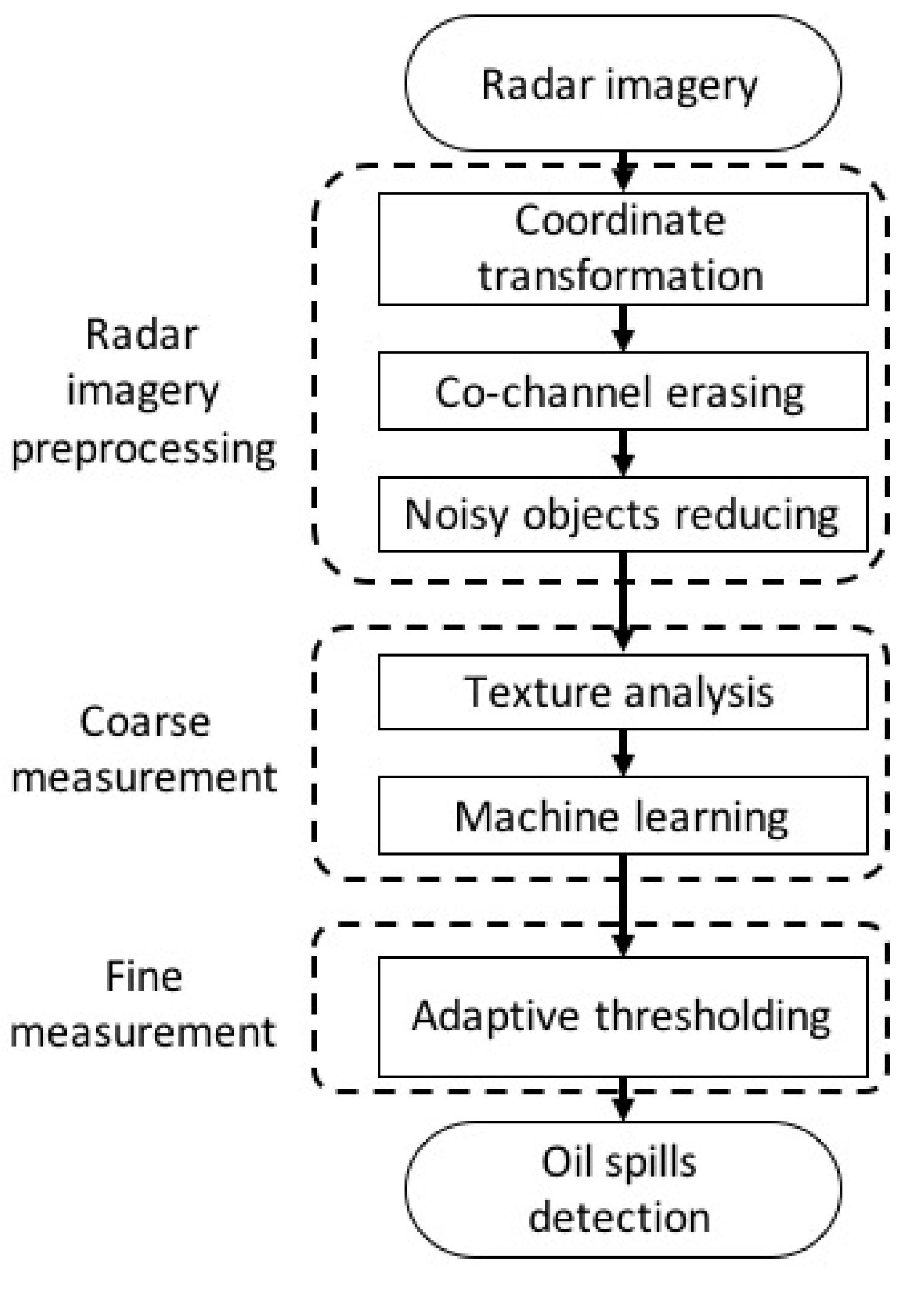
1. Introduction
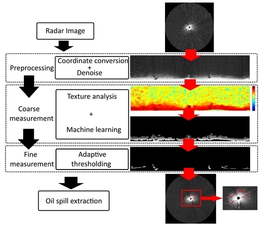
2. Radar Image Preprocessing
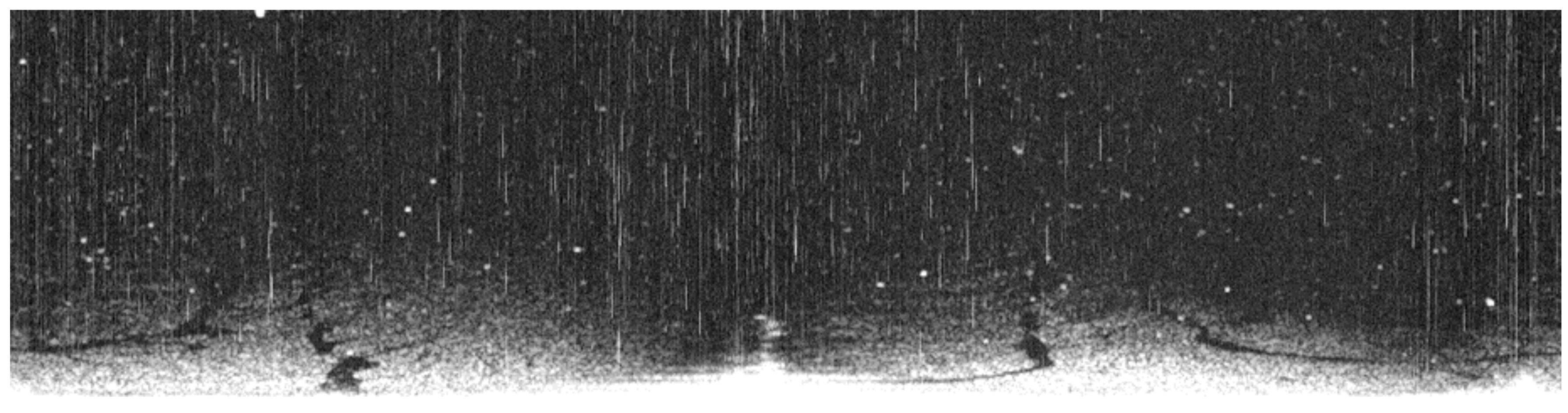
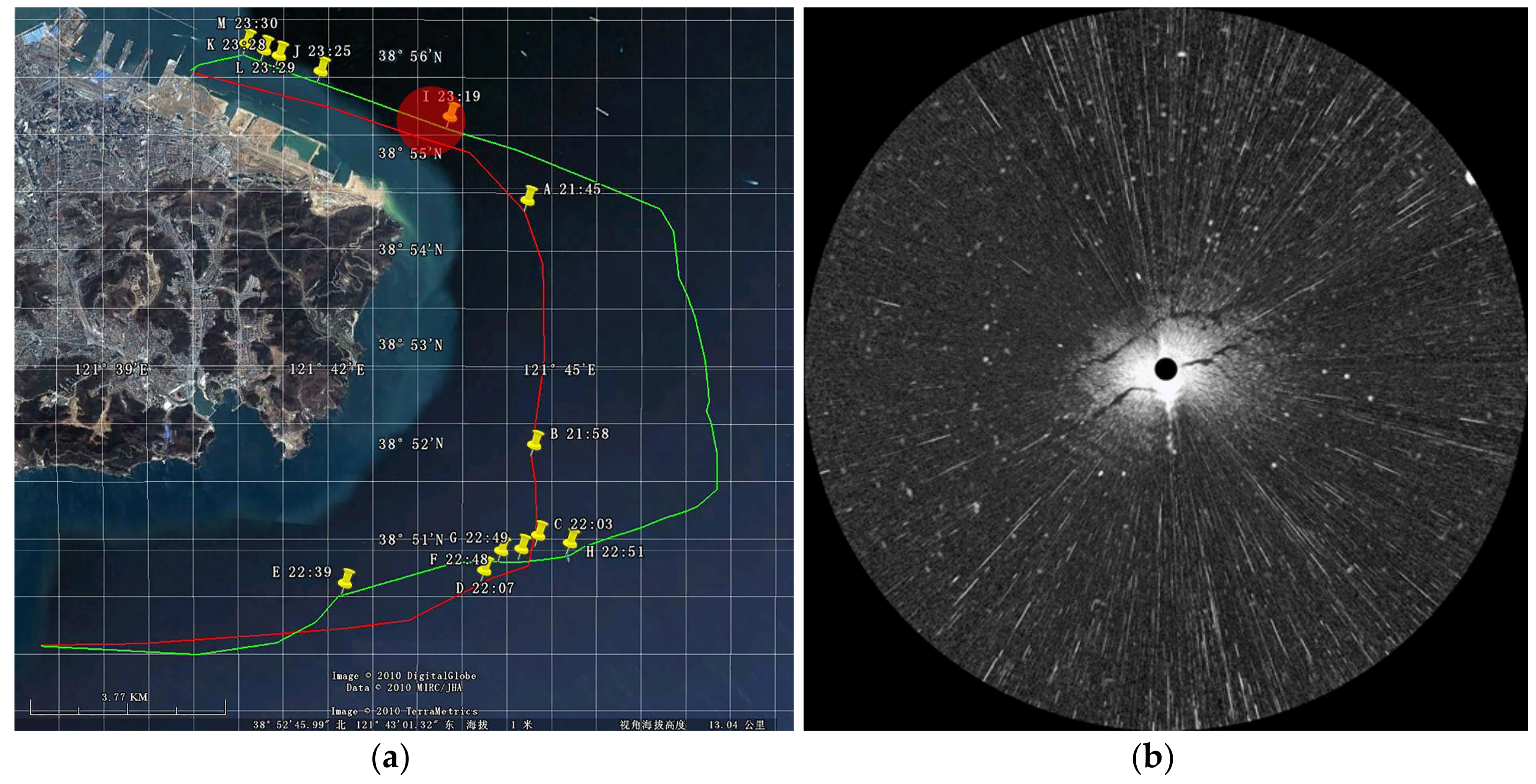
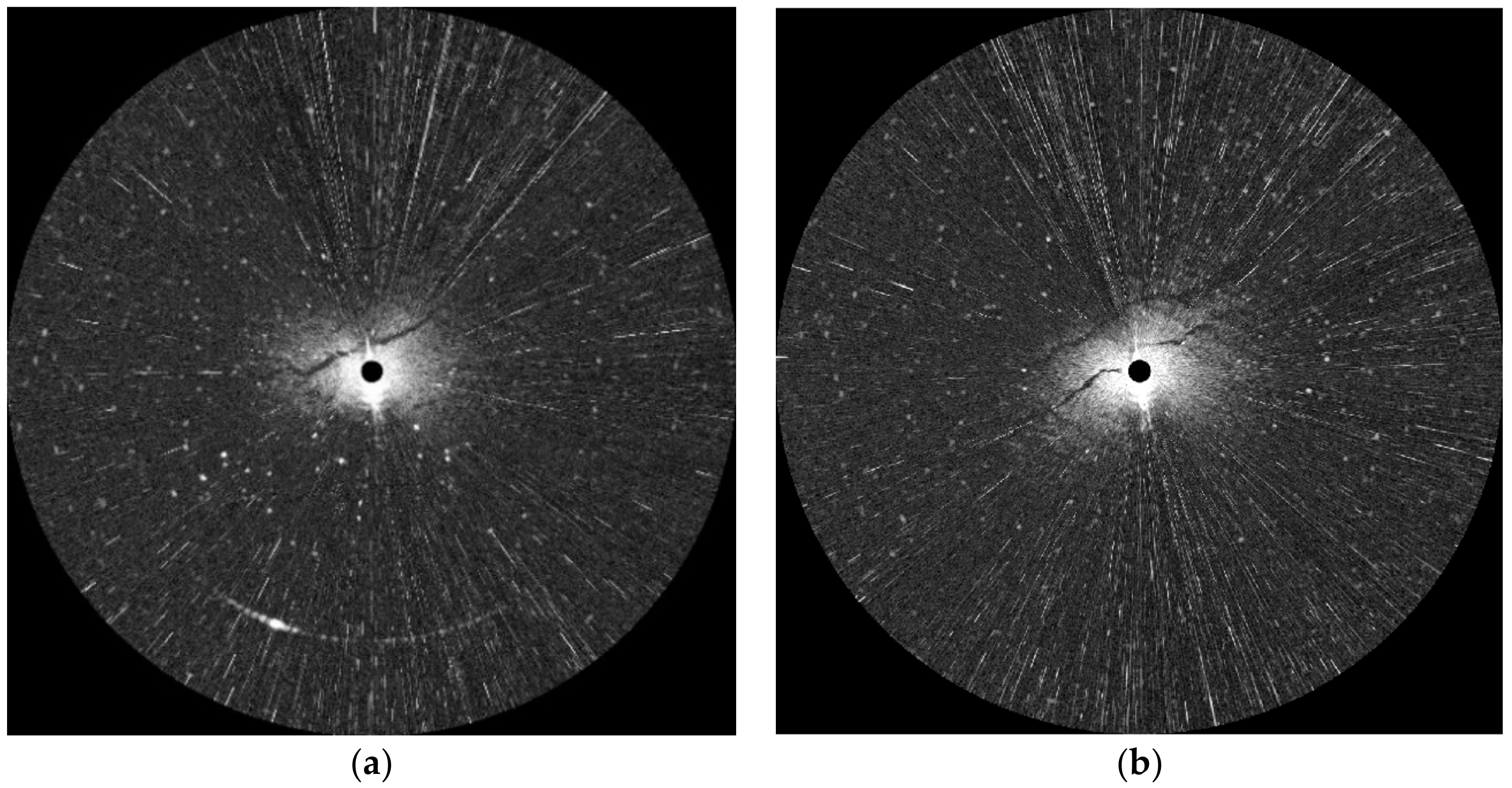
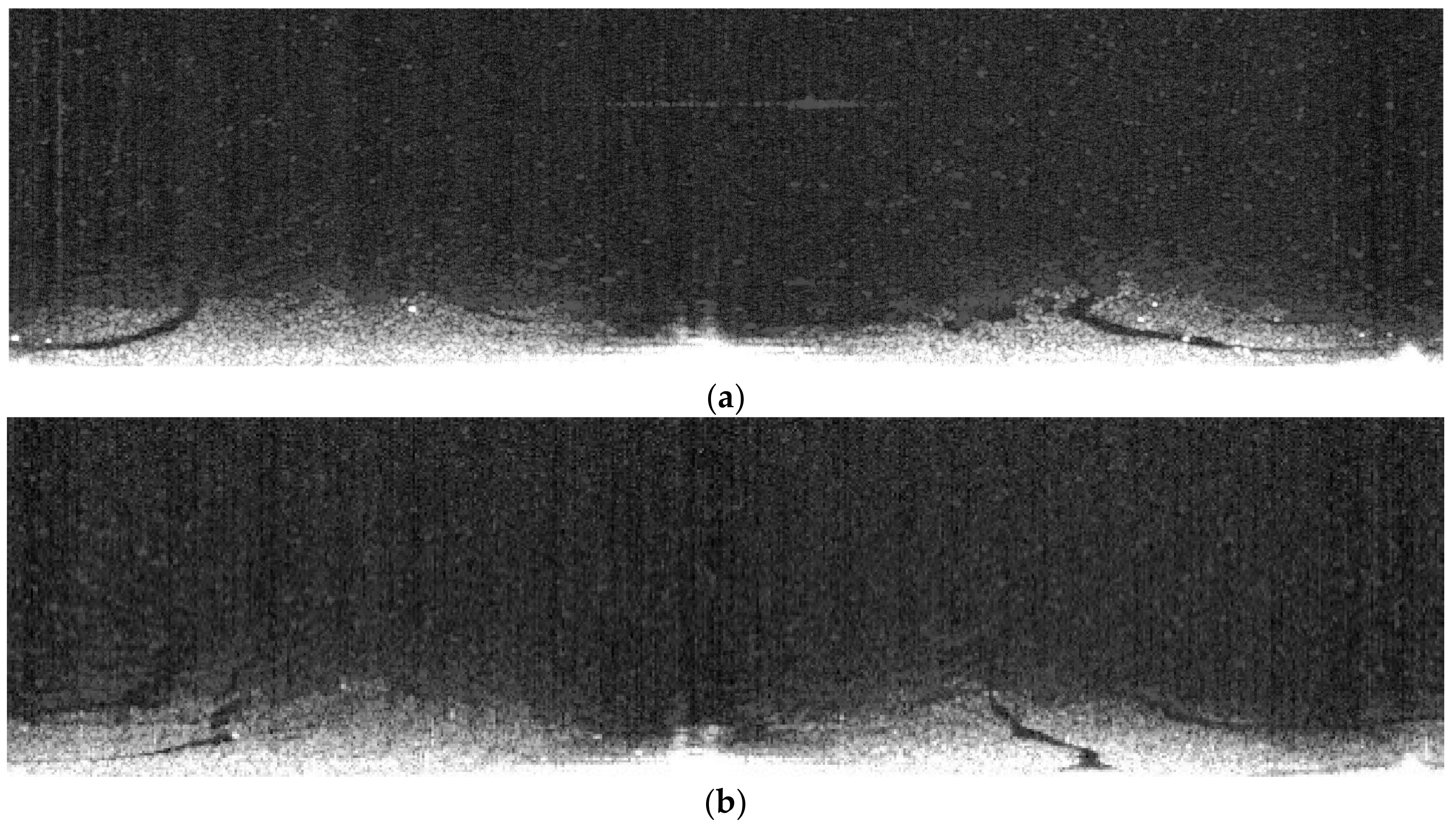
2.1. Radar Image Collection
2.2. Denoising
3. Coarse Measurement
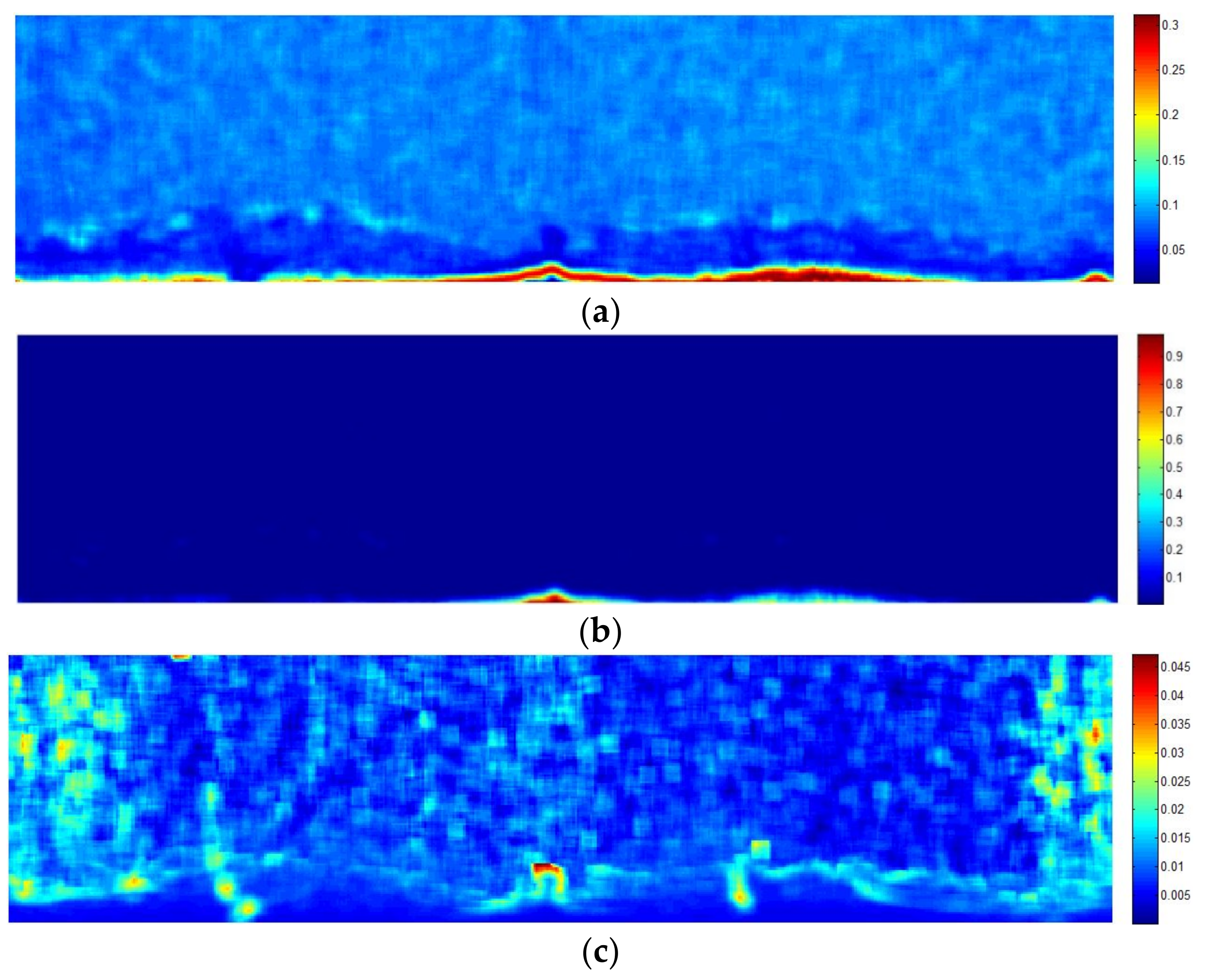
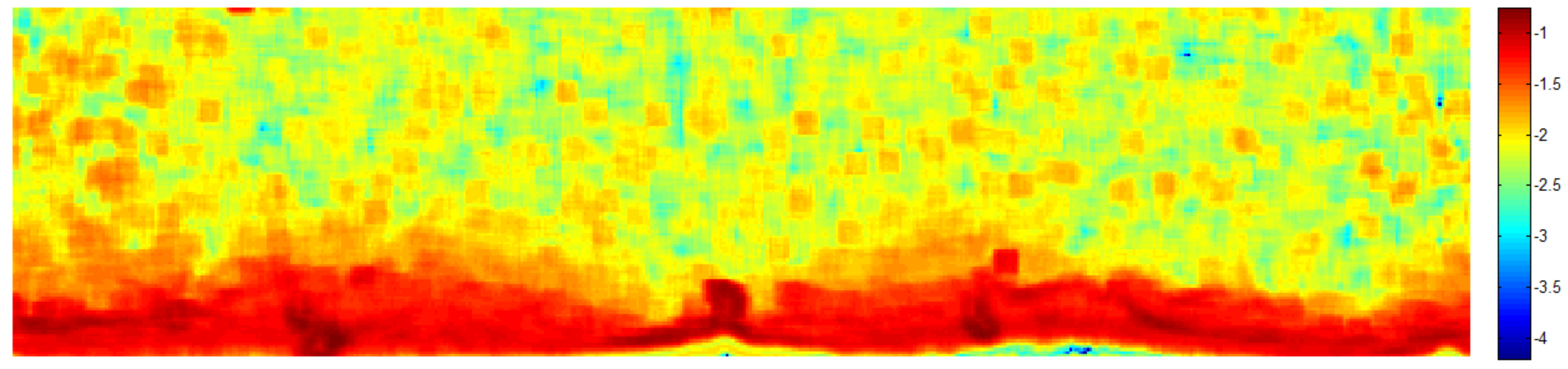
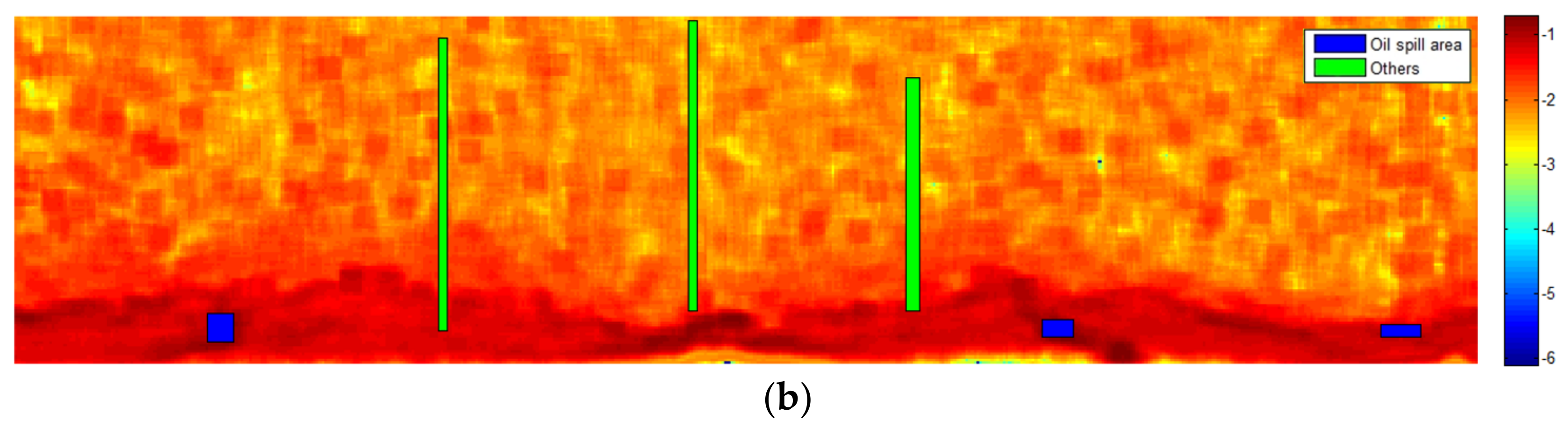
3.1. Texture Analysis
3.2. Classification by Machine Learning Algorithm
3.2.1. SVM
3.2.2. k-NN
3.2.3. LDA
3.2.4. Ensemble Learning (EL)
3.2.5. Oil Spill Detection on the Texture Analyzed Image
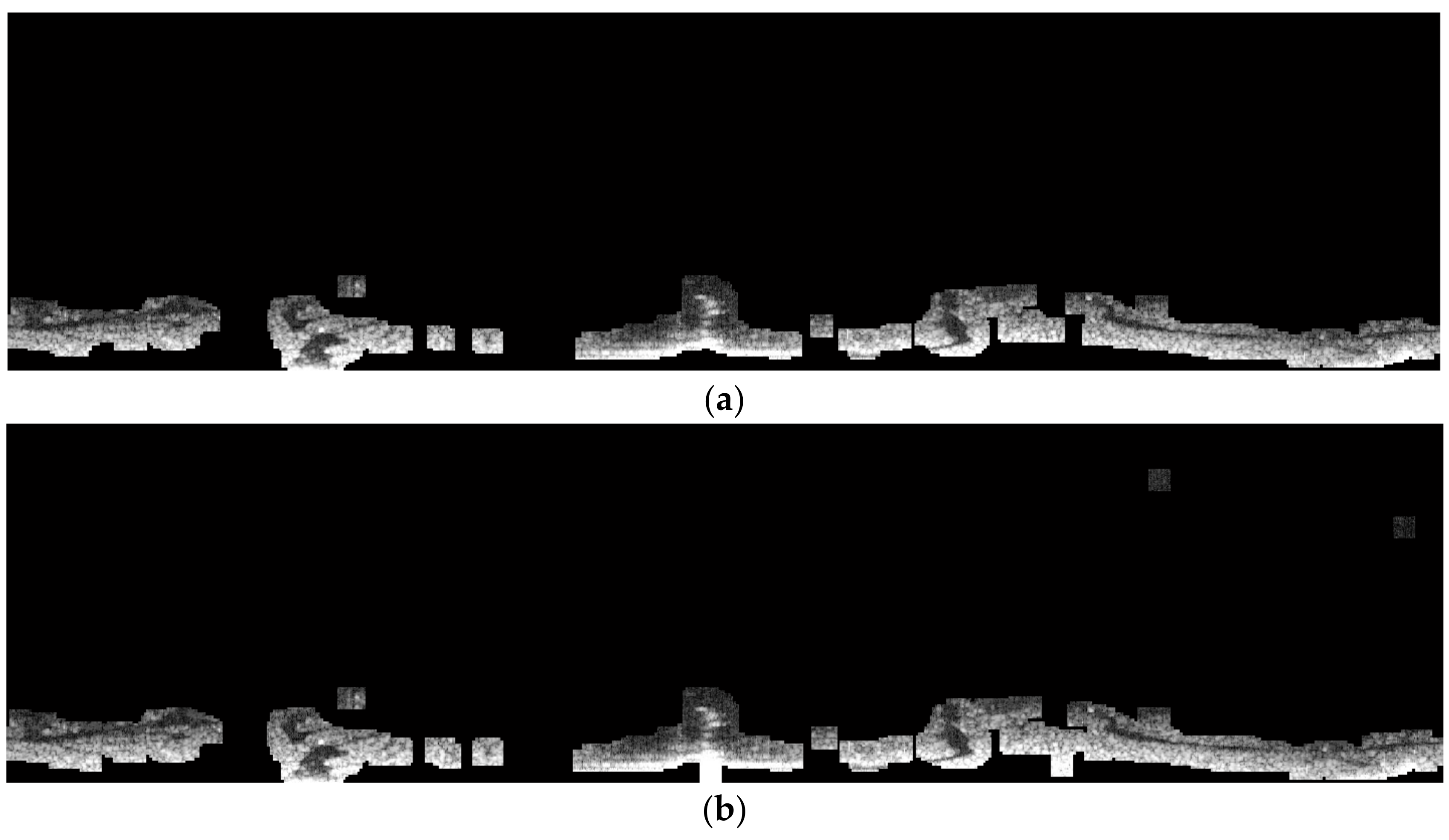
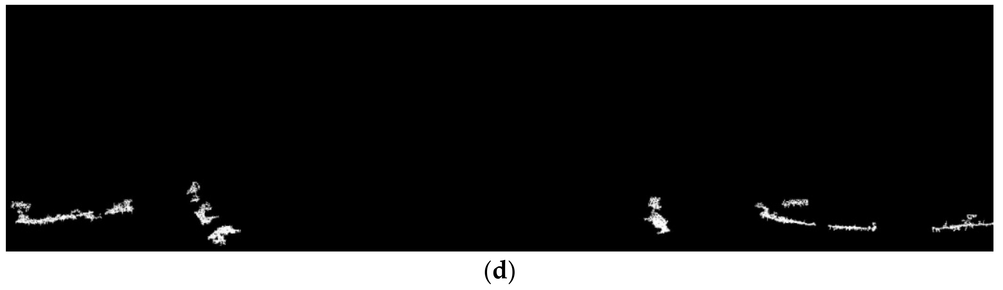
4. Fine Measurements
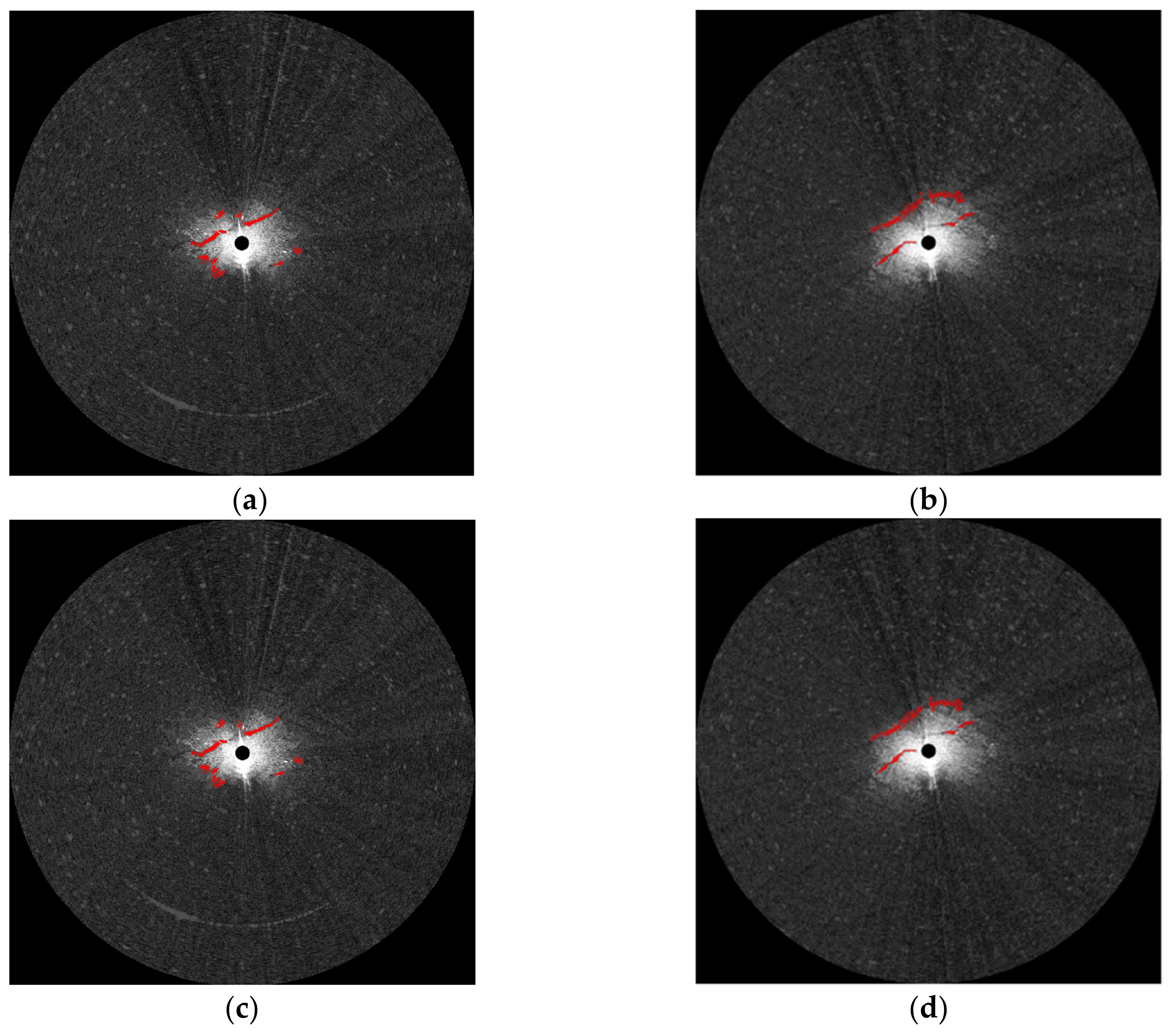
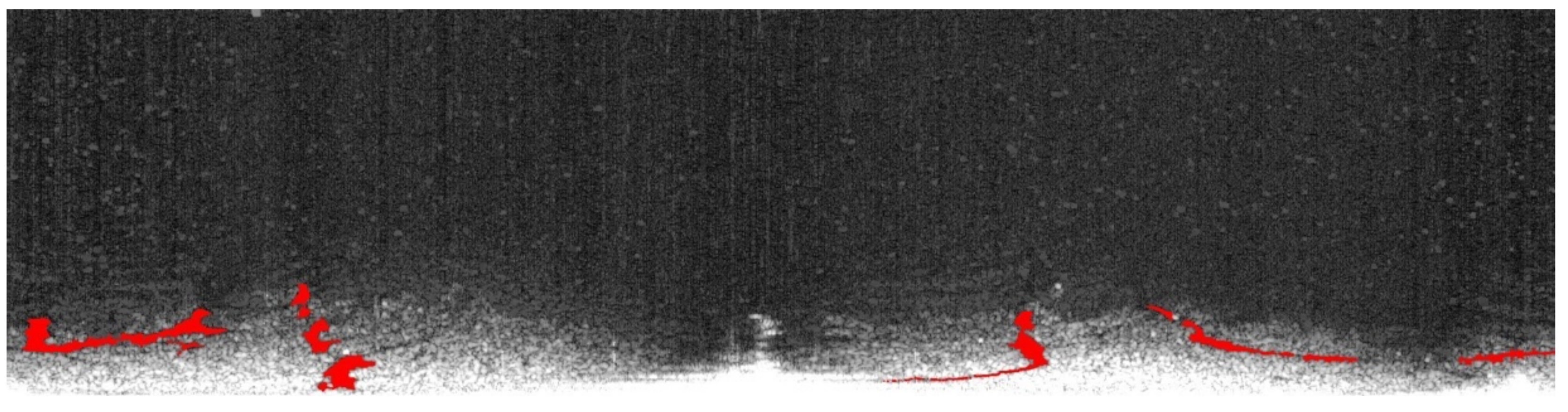
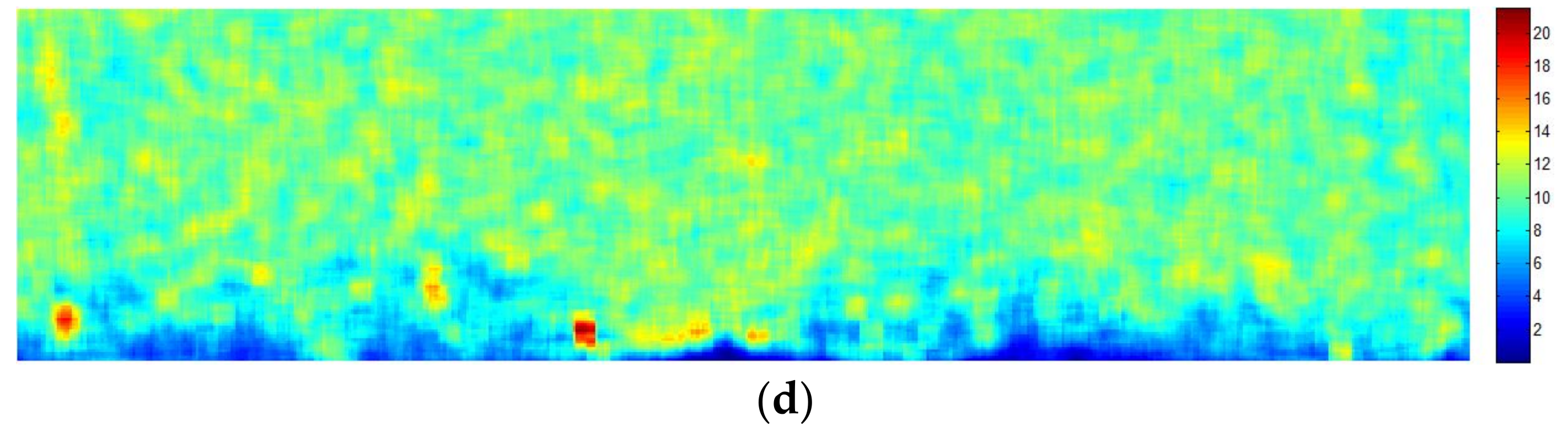
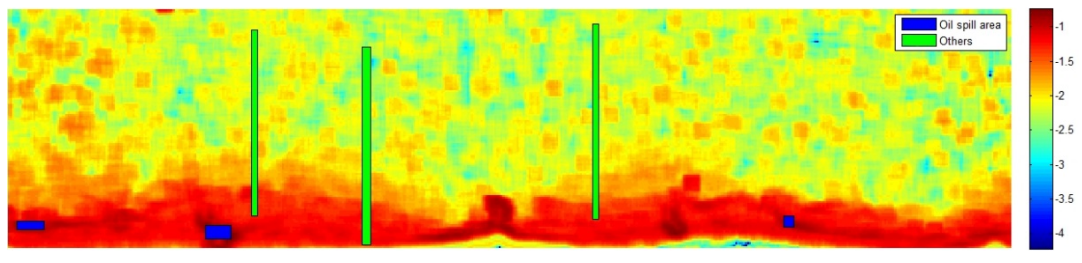
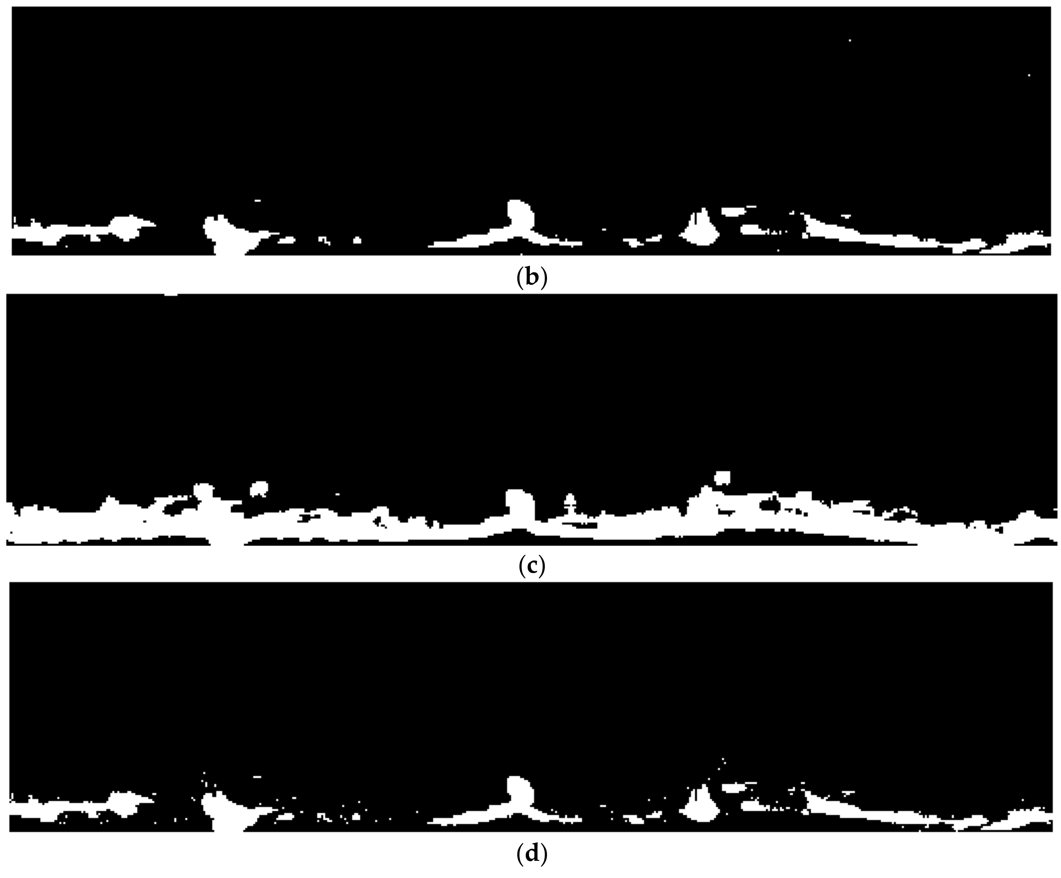
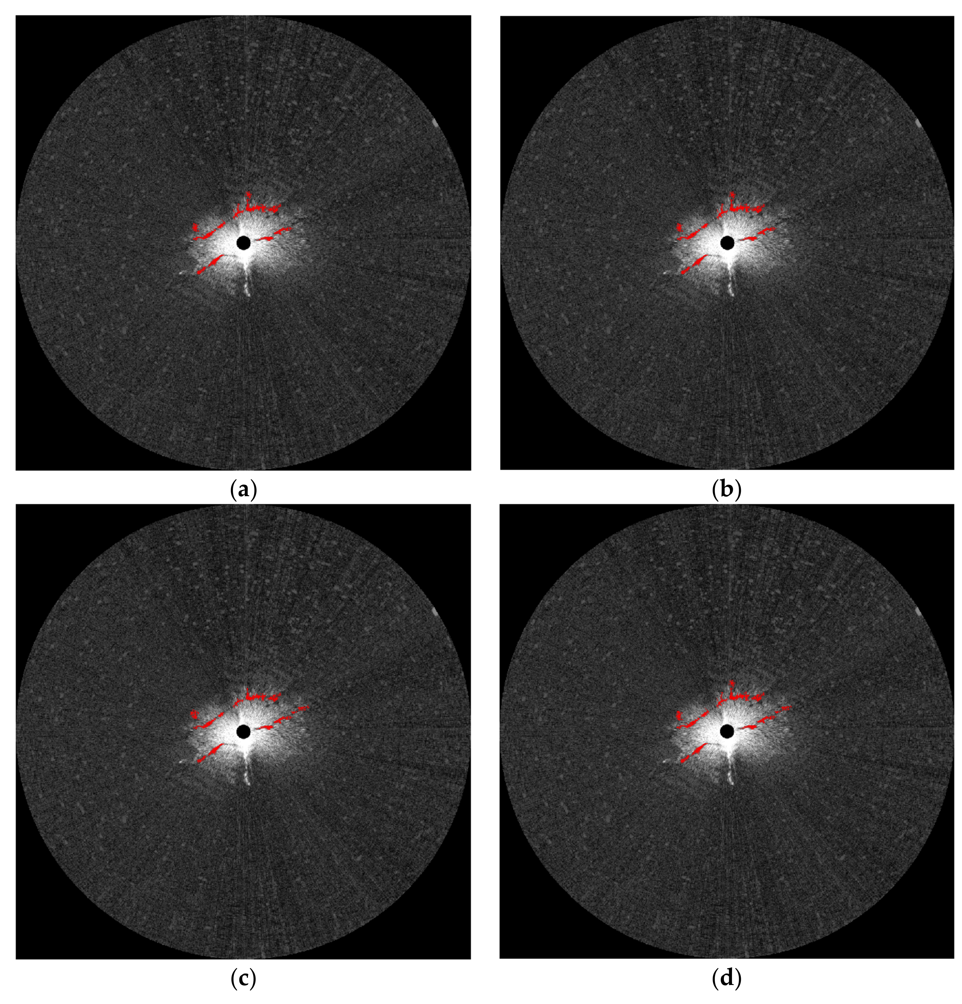
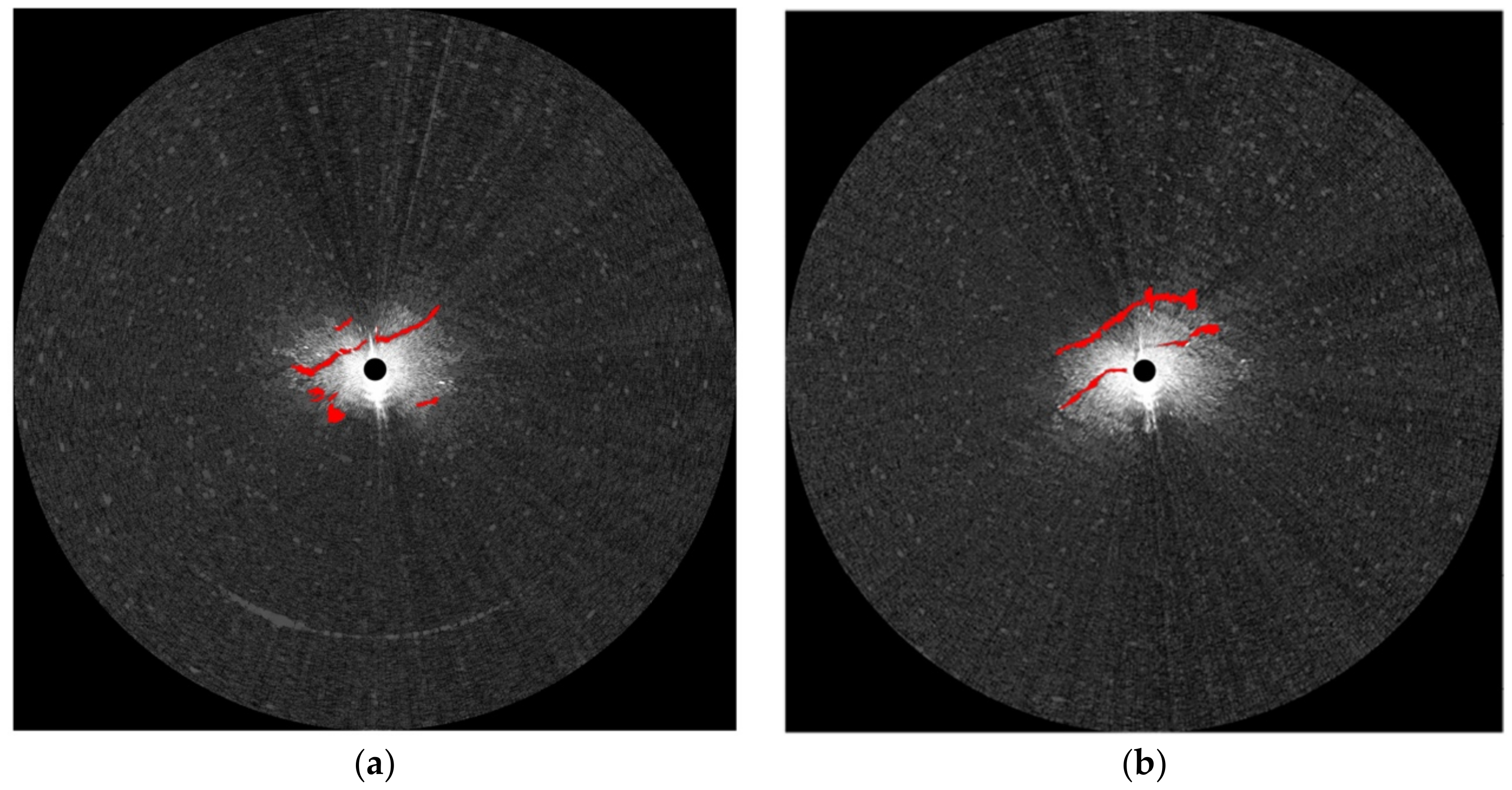
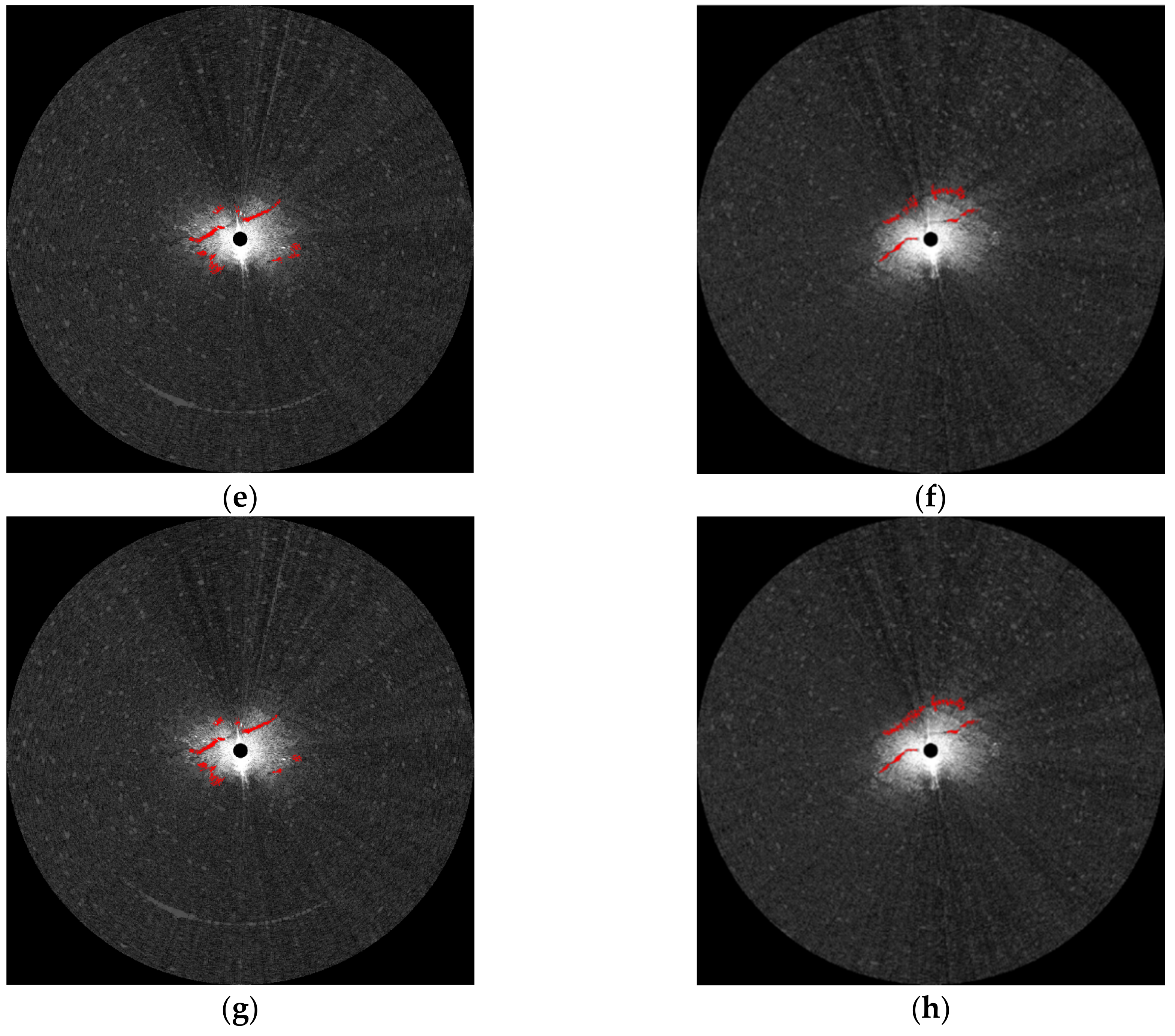
5. Results
6. Discussion
7. Conclusions
Author Contributions
Funding
Acknowledgments
Conflicts of Interest
References
- Lardner, R.; Zodiatis, G. Modelling oil plumes from subsurface spills. Mar. Pollut. Bull. 2017, 124, 94–101. [Google Scholar] [CrossRef]
- Alves, T.M.; Kokinou, E.; Zodiatis, G.; Radhakrishnan, H.; Panagiotakis, C.; Lardner, R. Multidisciplinary oil spill modeling to protect coastal communities and the environment of the Eastern Mediterranean Sea. Sci. Rep. 2016, 6, 36882. [Google Scholar] [CrossRef] [PubMed]
- Alves, T.M.; Kokinou, E.; Zodiatis, G.; Lardner, R.; Panagiotakis, C.; Radhakrishnan, H. Modelling of oil spills in confined maritime basins: The case for early response in the Eastern Mediterranean Sea. Environ. Pollut. 2015, 206, 390–399. [Google Scholar] [CrossRef] [PubMed]
- Alves, T.M.; Kokinou, E.; Zodiatis, G. A three-step model to assess shoreline and offshore susceptibility to oil spills: The South Aegean (Crete) as an analogue for confined marine basins. Mar. Pollut. Bull. 2014, 86, 443–457. [Google Scholar] [CrossRef]
- Delpeche-Ellmann, N.C.; Soomere, T. Investigating the marine protected areas most at risk of current-driven pollution in the Gulf of Finland, the Baltic Sea, using a Lagrangian transport model. Mar. Pollut. Bull. 2013, 67, 121–129. [Google Scholar] [CrossRef] [PubMed]
- International Maritime Organization. Appendix A: Extract from regulation 12. In Proceedings of the International Convention for the Safety of Life at Sea, London, UK, 1 November 1974. [Google Scholar]
- Atanassov, V.; Mladenov, L.; Rangelov, R.; Savchenko, A. Observation of oil slicks on the sea surface by using marine navigation radar. In Proceedings of the Remote Sensing, Global Monitoring for Earth Management: 1991 International Geoscience and Remote Sensing Symposium, Helsinki University of Technology, Espo, Finland, 3–6 June 1991; pp. 1323–1326. [Google Scholar]
- Nost, E.; Egset, C.N. Oil spill detection system—Results from field trials. In Proceedings of the OCEANS 2006, Boston, MA, USA, 18–21 September 2006. [Google Scholar]
- Gangeskar, R. Automatic oil-spill detection by marine X-band radars. Sea Technol. 2004, 45, 40–45. [Google Scholar]
- SeaDarQ. Available online: http://www.seadarq.com/seadarq/products/oil-spill-detection-1 (accessed on 30 December 2018).
- Rutter. Available online: http://www.rutter.ca/oil-spill-detection (accessed on 30 December 2018).
- Bartsch, N.; Gruner, K.; Keydel, W.; Witte, F. Contributions to oil-spill detection and analysis with radar and microwave radiometry: Results of the archimedes II campaign. IEEE Trans. Geosci. Remote Sens. 1987, 25, 677–690. [Google Scholar] [CrossRef]
- Tennyson, E.J. Shipboard navigational radar as an oil spill tracking tool-a preliminary assessment. In Proceedings of the IEEE OCEANS 1988, Baltimore, MD, USA, 31 October–2 November 1988. [Google Scholar]
- Zhu, X.; Li, Y.; Feng, H.; Liu, B.; Xu, J. Oil spill detection method using X-band marine radar imagery. J. Appl. Remote Sens. 2015, 9, 123–129. [Google Scholar] [CrossRef]
- Liu, P.; Li, Y.; Xu, J.; Zhu, X. Adaptive enhancement of X-band marine radar imagery to detect oil spill segments. Sensors 2017, 17, 2349. [Google Scholar]
- Xu, J.; Liu, P.; Wang, H.; Lian, J.; Li, B. Marine radar oil spill monitoring technology based on dual-threshold and c–v level set methods. J. Indian Soc. Remote. 2018, 46, 1949–1961. [Google Scholar] [CrossRef]
- Otsu, N. Threshold selection method from gray-level histograms. IEEE Trans. Syst. Man Cybern. 1979, 9, 62–66. [Google Scholar] [CrossRef]
- Sezgin, M.; Sankur, B. Survey over image thresholding techniques and quantitative performance evaluation. J. Electron. Imaging 2004, 13, 146–165. [Google Scholar]
- Kundu, A.; Mitra, S.K.; Vaidyanathan, P.P. Application of two-dimensional generalized mean filtering for removal of impulse noises from images. IEEE Trans. Acoust. Speech 1984, 32, 600–609. [Google Scholar] [CrossRef]
- Roth, S.; Black, M.J. Fields of Experts. Int. J. Comput. Vis. 2009, 82, 205–229. [Google Scholar] [CrossRef]
- Akar, S.; Mehmet, L.S.; Kaymakci, N. Detection and object-based classification of offshore oil slicks using ENVISAT-ASAR images. Environ. Monit. Assess. 2011, 183, 409–423. [Google Scholar] [CrossRef] [PubMed]
- Tamura, H.; Mori, S.; Yamawaki, T. Textural features corresponding to visual perception. IEEE Trans. Syst. Man Cybern. 1978, 8, 460–473. [Google Scholar] [CrossRef]
- Haralick, R.M. Statistical and structural approaches to texture. Proc. IEEE 1979, 67, 786–804. [Google Scholar] [CrossRef]
- Mahmoud, A.; Elbialy, S.; Pradhan, B.; Buchroithner, M. Field-based landcover classification using TerraSAR-X texture analysis. Adv. Space Res. 2011, 48, 799–805. [Google Scholar] [CrossRef]
- Lee, M.A.; Aanstoos, J.V.; Bruce, L.M.; Prasad, S. Application of omnidirectional texture analysis to SAR images for levee landslide detection. In Proceedings of the 2012 IEEE International Geoscience and Remote Sensing Symposium (IGARSS), Munich, Germany, 22–27 July 2012. [Google Scholar]
- Wei, L.; Hu, Z.; Guo, M.; Jiang, M.; Zhang, S. Texture feature analysis in oil spill monitoring by SAR image. In Proceedings of the 20th International Conference on Geoinformatics, Hong Kong, China, 15–17 June 2012. [Google Scholar]
- Nghiem, S.V.; Li, F.K.; Lou, S.H.; Neumann, G. Ocean remote sensing with airborne Ku-band scatterometer. In Proceedings of the OCEANS’93, Victoria, BC, Canada, 18–21 October 1993; pp. 120–124. [Google Scholar]
- Schroeder, L.; Schaffner, P.; Mitchell, J.; Jones, W. AAFE RADSCAT 13.9-GHz measurements and analysis: Wind-speed signature of the ocean. IEEE J. Ocean. Eng. 1985, 10, 346–357. [Google Scholar] [CrossRef]
- Ulaby, F.T.; Kouyate, F.; Brisco, B.; Williams, T.H.L. Textural infornation in SAR images. IEEE Trans. Geosci. Remote Sens. 1986, 24, 235–245. [Google Scholar] [CrossRef]
- Jaähne, B. Digital Image Processing, 6th ed.; Springer: Berlin, Germany, 2005; p. 78. [Google Scholar]
- David, A.; Lerner, B. Support vector machine-based image classification for genetic syndrome diagnosis. Pattern Recogn. Lett. 2005, 26, 1029–1038. [Google Scholar] [CrossRef]
- Wang, X.Y.; Wang, Q.Y.; Yang, H.Y.; Bu, J. Color image segmentation using automatic pixel classification with support vector machine. Neurocomputing 2011, 74, 3898–3911. [Google Scholar] [CrossRef]
- Wang, X.Y.; Zhang, X.J.; Yang, H.Y.; Bu, J. A pixel-based color image segmentation using support vector machine and fuzzy C-means. Neural Netw. 2012, 33, 148–159. [Google Scholar] [CrossRef] [PubMed]
- Burges, C.J.C. A tutorial on support vector machines for pattern recognition. Data Min. Knowl. Disc. 1998, 2, 121–167. [Google Scholar] [CrossRef]
- Samworth, R.J. Optimal weighted nearest neighbour classifiers. Ann. Stat. 2012, 40, 2733–2763. [Google Scholar] [CrossRef]
- Decaestecker, C.; Salmon, I.; Dewitte, O.; Camby, I.; Ham, V.; Pasteels, J.L.; Brotchi, J.; Kiss, R. Nearest-neighbor classification for identification of aggressive versus nonaggressive low-grade astrocytic tumors by means of image cytometry-generated variables. J. Neurosurg. 1997, 86, 532–537. [Google Scholar] [CrossRef] [PubMed]
- Ng, M.K.; Liao, L.Z.; Zhang, L. On sparse linear discriminant analysis algorithm for high-dimensional data classification. Numer. Linear Algebra Appl. 2011, 18, 223–235. [Google Scholar] [CrossRef]
- Peng, J.; Luo, T. Sparse matrix transform-based linear discriminant analysis for hyperspectral image classification. Signal Image Video 2016, 10, 761–768. [Google Scholar] [CrossRef]
- Ye, Q.; Ye, N.; Yin, T. Fast orthogonal linear discriminant analysis with application to image classification. Neurocomputing 2015, 158, 216–224. [Google Scholar] [CrossRef]
- Samat, A.; Du, P.; Baig, M.H.A.; Chakravarty, S.; Cheng, L. Ensemble learning with multiple classifiers and polarimetric features for polarized SAR image classification. Photogramm. Eng. Rem. 2014, 80, 239–251. [Google Scholar] [CrossRef]
- Wu, Q.; Wang, L.W.; Wu, J. Ensemble learning on hyperspectral remote sensing image classification. Adv. Mater. Res. 2012, 546–547, 508–513. [Google Scholar] [CrossRef]
- Merentitis, A.; Debes, C.; Heremans, R. Ensemble learning in hyperspectral image classification: Toward selecting a favorable bias-variance tradeoff. IEEE J.-STARS 2014, 7, 1089–1102. [Google Scholar] [CrossRef]
- Niblack, W. An Introduction to Digital Image Processing; Prentice Hall: Upper Saddle River, NJ, USA, 1986. [Google Scholar]
- Sauvola, J.; Pietikäinen, M. Adaptive document image binarization. Pattern Recognit. 2000, 33, 225–236. [Google Scholar] [CrossRef]
- White, J.M.; Rohrer, G.D. Image thresholding for optical character recognition and other applications requiring character image extraction. IBM J. Res. Dev. 1983, 27, 400–411. [Google Scholar] [CrossRef]
- Yanowitz, S.D.; Bruckstein, A.M. A new method for image segmentation. Comput. Graph. Image Process. 1989, 46, 82–95. [Google Scholar] [CrossRef]
- Wall, R.J. The Gray Level Histogram for Threshold Boundary Determination in Image Processing to the Scene Segmentation Problem in Human Chromosome Analysis. Ph.D. Thesis, University of California at Los Angeles, Los Angeles, CA, USA, 1974. [Google Scholar]
- Bradley, D.; Roth, G. Adaptive thresholding using the Integral Image. J. Graph. Tools 2007, 12, 13–21. [Google Scholar] [CrossRef]


| Name | Parameters |
|---|---|
| Working frequency | 9.41 GHz |
| Antenna length | 8 ft |
| Detection range | 0.5–12 nautical miles |
| Horizontal direction | 360 |
| Vertical direction | 10 |
| Peak power | 25 kW |
| Pulse width | 50 ns/250 ns/750 ns |
| Pulse repetition frequency | 3000 Hz/1800 Hz/785 Hz |
| Machine Learning Methods | |||||
|---|---|---|---|---|---|
| SVM | k-NN | LDA | EL | ||
| 0.10 | 0.3014 | 0.2899 | 0.1744 | 0.2494 | |
| 0.8788 | 0.8833 | 0.9496 | 0.9287 | ||
| 0.15 | 0.3574 | 0.3411 | 0.2189 | 0.3122 | |
| 0.8771 | 0.8815 | 0.9278 | 0.927 | ||
| 0.20 | 0.4403 | 0.4351 | 0.3169 | 0.4105 | |
| 0.8462 | 0.8506 | 0.9161 | 0.896 | ||
| 0.25 | 0.5176 | 0.5111 | 0.4315 | 0.4972 | |
| 0.8215 | 0.8348 | 0.8809 | 0.88 | ||
| 0.30 | 0.6184 | 0.6143 | 0.582 | 0.6338 | |
| 0.805 | 0.8053 | 0.8719 | 0.8623 | ||
| 0.35 | 0.8009 | 0.813 | 0.876 | 0.8096 | |
| 0.7782 | 0.7788 | 0.7936 | 0.8161 | ||
| 0.40 | 0.9485 | 0.9484 | 0.9597 | 0.9583 | |
| 0.6632 | 0.6641 | 0.547 | 0.6237 | ||
| 0.45 | 0.9738 | 0.9736 | 0.972 | 0.9713 | |
| 0.5032 | 0.5035 | 0.4597 | 0.4651 | ||
| 0.50 | 0.9766 | 0.9763 | 0.9762 | 0.9764 | |
| 0.3685 | 0.3682 | 0.318 | 0.3547 | ||
| Configuration | Type |
|---|---|
| CPU | Inter® Core™ i5-4300U |
| Memory | 8 GB |
| Display card | Intel HD Graphics 4400 |
| Hard disc | Solid State Drive 128 GB |
© 2019 by the authors. Licensee MDPI, Basel, Switzerland. This article is an open access article distributed under the terms and conditions of the Creative Commons Attribution (CC BY) license (http://creativecommons.org/licenses/by/4.0/).
Share and Cite
Liu, P.; Li, Y.; Liu, B.; Chen, P.; Xu, J. Semi-Automatic Oil Spill Detection on X-Band Marine Radar Images Using Texture Analysis, Machine Learning, and Adaptive Thresholding. Remote Sens. 2019, 11, 756. https://doi.org/10.3390/rs11070756
Liu P, Li Y, Liu B, Chen P, Xu J. Semi-Automatic Oil Spill Detection on X-Band Marine Radar Images Using Texture Analysis, Machine Learning, and Adaptive Thresholding. Remote Sensing. 2019; 11(7):756. https://doi.org/10.3390/rs11070756
Chicago/Turabian StyleLiu, Peng, Ying Li, Bingxin Liu, Peng Chen, and Jin Xu. 2019. "Semi-Automatic Oil Spill Detection on X-Band Marine Radar Images Using Texture Analysis, Machine Learning, and Adaptive Thresholding" Remote Sensing 11, no. 7: 756. https://doi.org/10.3390/rs11070756
APA StyleLiu, P., Li, Y., Liu, B., Chen, P., & Xu, J. (2019). Semi-Automatic Oil Spill Detection on X-Band Marine Radar Images Using Texture Analysis, Machine Learning, and Adaptive Thresholding. Remote Sensing, 11(7), 756. https://doi.org/10.3390/rs11070756