Towards a Long-Term Reanalysis of Land Surface Variables over Western Africa: LDAS-Monde Applied over Burkina Faso from 2001 to 2018

Abstract

This study focuses on the ability of the global Land Data Assimilation System, LDAS-Monde, to improve the representation of land surface variables (LSVs) over Burkina-Faso through the joint assimilation of satellite derived surface soil moisture (SSM) and leaf area index (LAI) from January 2001 to June 2018. The LDAS-Monde offline system is forced by the latest European Centre for Medium-Range Weather Forecasts (ECMWF) atmospheric reanalysis ERA5 as well as ERA-Interim former reanalysis, leading to reanalyses of LSVs at 0.25° × 0.25° and 0.50° × 0.50° spatial resolution, respectively. Within LDAS-Monde, SSM and LAI observations from the Copernicus Global Land Service (CGLS) are assimilated with a simplified extended Kalman filter (SEKF) using the CO2-responsive version of the ISBA (Interactions between Soil, Biosphere, and Atmosphere) land surface model (LSM). First, it is shown that ERA5 better represents precipitation and incoming solar radiation than ERA-Interim former reanalysis from ECMWF based on in situ data. Results of four experiments are then compared: Open-loop simulation (i.e., no assimilation) and analysis (i.e., joint assimilation of SSM and LAI) forced by either ERA5 or ERA-Interim. After jointly assimilating SSM and LAI, it is noticed that the assimilation is able to impact soil moisture in the first top soil layers (the first 20 cm), and also in deeper soil layers (from 20 cm to 60 cm and below), as reflected by the structure of the SEKF Jacobians. The added value of using ERA5 reanalysis over ERA-Interim when used in LDAS-Monde is highlighted. The assimilation is able to improve the simulation of both SSM and LAI: The analyses add skill to both configurations, indicating the healthy behavior of LDAS-Monde. For LAI in particular, the southern region of the domain (dominated by a Sudan-Guinean climate) highlights a strong impact of the assimilation compared to the other two sub-regions of Burkina-Faso (dominated by Sahelian and Sudan-Sahelian climates). In the southern part of the domain, differences between the model and the observations are the largest, prior to any assimilation. These differences are linked to the model failing to represent the behavior of some specific vegetation species, which are known to put on leaves before the first rains of the season. The LDAS-Monde analysis is very efficient at compensating for this model weakness. Evapotranspiration estimates from the Global Land Evaporation Amsterdam Model (GLEAM) project as well as upscaled carbon uptake from the FLUXCOM project and sun-induced fluorescence from the Global Ozone Monitoring Experiment-2 (GOME-2) are used in the evaluation process, again demonstrating improvements in the representation of evapotranspiration and gross primary production after assimilation.

1. Introduction

An accurate representation of land surface variables (LSVs), such as soil moisture or vegetation cover, is critical in climate science as well as environmental monitoring and prediction (e.g., in order to cope with drought, flood, or other extreme events). To that end, land surface models (LSMs) have been widely used to simulate and predict the Earth’s water storage energy budgets over a broad range of time scales [1,2,3,4]. For instance, the AMMA (African Monsoon Multidisciplinary Analysis) Land Surface Model Intercomparison Project (ALMIP) used a set of LSMs forced in offline mode by a combination of satellite products and high quality in situ measurements in order to better apprehend LSV processes and their representation [5,6]. These LSMs are intended to reproduce LSVs, such as surface and root zone soil moisture (SSM and RZSM, respectively), vegetation biomass, and leaf area index (LAI), together with surface energy fluxes and streamflow simulations. Over the last two decades, much progress has been made on the degree to which realistic land surface initialization contributes to the skill and performance of subseasonal land-related predictability as documented by [7,8] in the Global Land-Atmosphere Coupling Experiment (GLACE). LSMs have subsequently benefited from the growing development of observational networks. Unfortunately, those are not evenly spaced and data sparse regions remain very difficult to model with accuracy. This is the case of West Africa ([5,9]), where LSVs are of primary importance, as emphasized by many studies, see, e.g., [10,11].

Representation of LSVs by LSMs can be improved through the dynamical integration of observations [12,13], and remote sensing observations are particularly useful in this context as they are now unrestrictedly available at a global scale with high spatial resolution and with long-term records. Land data assimilation systems (LDASs) combine LSMs with satellite observations in order to produce reanalyses of LSVs. Several LDASs now exist, amongst them are the Global Land Data Assimilation System (GLDAS, [1]), the Carbon Cycle Data Assimilation System (CCDAS, [14]), the Coupled Land Vegetation LDAS (CLVLDAS, [15,16,17]), the U.S. National Climate Assessment LDAS (NCA-LDAS, reference [18]) as well as LDAS-Monde [19] to name a few. More recently, soil moisture (SM) data from the Soil Moisture Operational Product System (SMOPS) has been assimilated in the Noah model [20]. Those systems either optimize process parameters (e.g., CCDAS), state variables (e.g., GLDAS, NCA-LDAS, LDAS-Monde), or both (e.g., CLVLDAS). Only few studies have considered the integration of multiple remote sensing measurements [17,19] and even less have had a specific focus over West Africa (e.g., [21]).

In this context, the present study aims to evaluate reanalyses of LSVs obtained with LDAS-Monde [19] over Burkina Faso in West Africa (domain shown in Figure 1). This country exhibits three distinctive climates: Sahel, Sudan-Sahel, and Sudan-Guinea that cover most part of West Africa, making Burkina Faso an area of interest for such study. A southward gradient characterizes rainfall distribution across the country: Mean annual precipitation decreases from more than 1100 mm in the South to approximately 300 mm in the North [22]. Daily mean temperature fluctuates between 21 and 34 °C (17 and 37 °C) during the rainy season (dry season) across Burkina Faso [23]. LDAS-Monde [19] is based on the CO₂-responsive version of the Interactions between Soil, Biosphere, and Atmosphere (ISBA) LSM [24,25,26,27] available through the SURFEX (SURFace EXternalisée; [28]) modelling system of Météo-France. The reanalysis is performed by assimilating jointly satellite-derived SSM and LAI using a simplified extended Kalman filter (SEKF). For that purpose, the most recent SURFEX_v8.1 Offline Data Assimilation (SODA) implementation has been utilized considering a long-term period (January 2001 to June 2018) along with the joint assimilation of both satellite-derived SSM (from 2007, [29]) and LAI (GEOV2, from 2001, http://land.copernicus.eu/global/, last access November 2018).

The quality of LSV reanalyses depends on the quality of LSMs and observations used, but also on the quality of atmospheric forcings used by LSMs. Numerous improvements were made in the generation of long-term (1979-onwards) global atmospheric reanalyses, leading to more advancements in land surface modeling fields and their applications (e.g., water resources monitoring [2,30,31]. In line with those improvements, NASA’s (National Aeronautics and Space Administration) Modern Era Retrospective analysis for Research and Applications (MERRA; [32], and MERRA2; [33]) as well as ECMWF’s (European Centre for Medium-Range Weather Forecasts) Interim reanalysis (ERA-Interim; [34]) were the most investigated. We take advantage of the recent development of ERA5, which was released in 2017 as the fifth generation of ECMWF global atmospheric reanalyses. At the time of this study, a time-slice of the ERA5 database was available from 2001 within 3 months of real time. ERA5 brings extensive changes compared to ERA-Interim, including higher spatial and temporal resolutions as well as a generally improved representation of, e.g., precipitation and incoming solar radiation (SW_in) [4,35,36]. The performance of ERA5 and ERA-Interim precipitation and SW_in is first investigated using in situ measurements over Burkina Faso (BF) before studying the quality of LDAS-Monde renalysis of LSVs forced by either ERA5 or ERA-interim.

Section 2 provides (i) a description of LDAS-Monde, including details on the CO₂-responsive version of the ISBA LSM and the data assimilation system, (ii) information on the atmospheric reanalyses used to force the system, the assimilated remotely sensed observations along with the in-situ and satellite datasets used to assess the sensitivity of the results to the atmospheric reanalysis, and (iii) the experimental set up and the evaluation strategies. Section 3 presents the results of a performance assessment of the reanalyses against in situ measurements, the assimilation impact of the assimilated variables as well as independent satellite datasets, and Section 4 provides perspectives and future directions.

2. Materials and Methods

2.1. LDAS-Monde

The LDAS [37,38,39,40,41], developed at Météo France’s Centre National de Recherches Météorologiques (CNRM), allows the integration of satellite-derived products into the ISBA LSM using a data assimilation scheme. It has been recently expanded to global scale (i.e., LDAS-Monde) [19,42,43]. LDAS-Monde is accessible through the open-access SURFEX modelling platform [28] (https://www.umr-cnrm.fr/surfex, last accessed January 2019). The following subsections briefly recall the main components of LDAS-Monde. More details can be found in [19].

2.1.1. ISBA Land Surface Model

In this paper, the CO₂-responsive [19,42,43] version of ISBA is used as well as the itsmulti-layer soil water and heat transfer [44,45] version. The soil is discretized with 14 layers spanning a 12 m depth. The lower boundary of each layer is 0.01, 0.04, 0.1, 0.2, 0.4, 0.6, 0.8, 1.0, 1.5, 2.0, 3.0, 5.0, 8.0, and 12 m deep (see Figure 1 of [45]). In this configuration, ISBA describes the water and carbon fluxes on a subdaily frequency, plant growth and crucial variables of vegetation components, such as LAI, and above ground-biomass.

In the ISBA model, the evolution of vegetation variables is controlled by photosynthesis, which enables vegetation growth resulting from the CO₂ uptake. A minimum LAI threshold is prescribed as 1 m²·m⁻² for coniferous forest or 0.3 m²·m⁻² for other vegetation types. Conversely, a lack of photosynthesis triggers higher mortality rates. The carbon uptake related to photosynthesis represents the gross primary production (GPP) while the CO₂ released by the soil-plant system constitutes the ecosystem respiration (RECO). The difference between these two quantities corresponds to the net ecosystem CO₂ exchange (NEE).

In the model version used in this study, ISBA parameters are prescribed for 12 generic land surface types, which consist of (i) nine plant functional types (needle leaf trees, evergreen broadleaf trees, deciduous broadleef trees, C3 crops, C4 crops, C4 irrigated crops, herbaceous, tropical herbaceous and wetlands), (ii) bare soil, (iii) rocks, and (iv) permanent snow and ice surfaces. Those parameters are derived from the ECOCLIMAP land cover database [46].

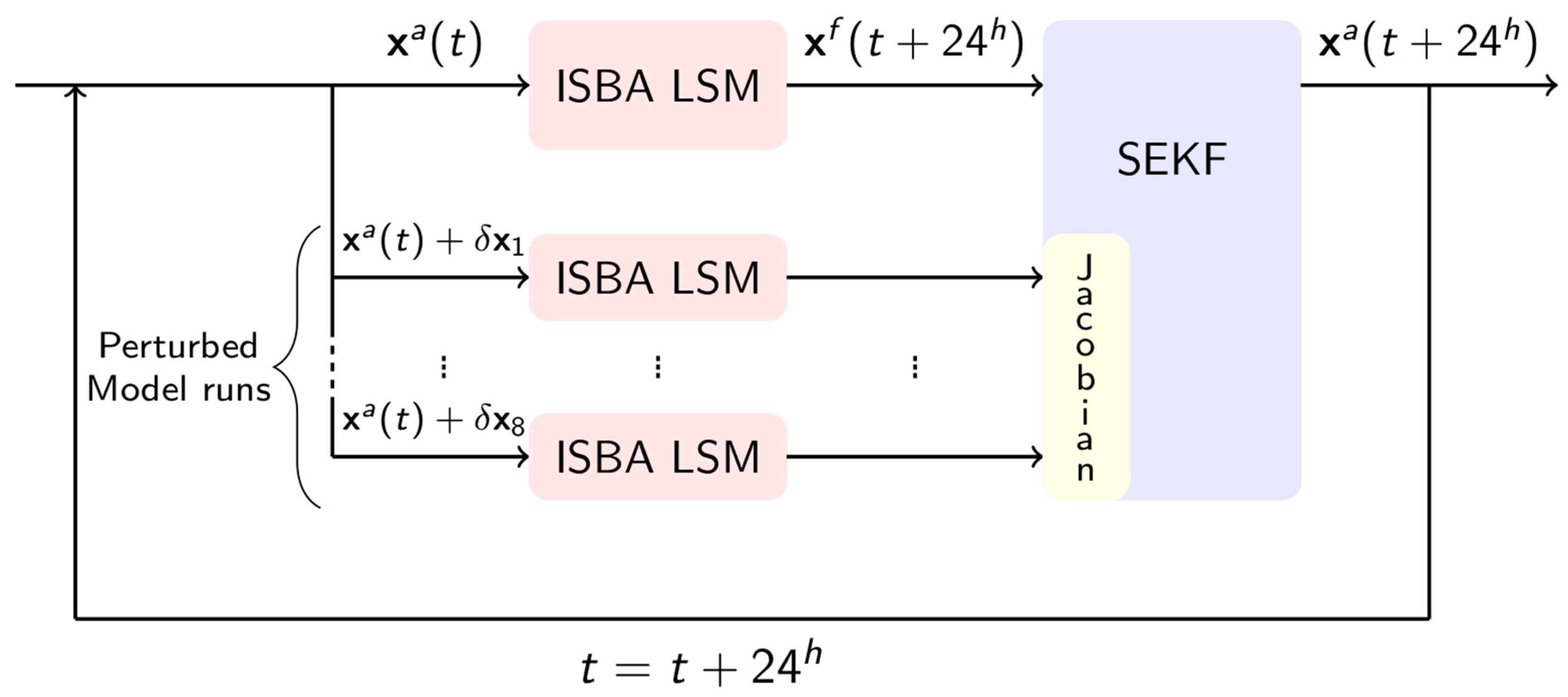
2.1.2. Data Assimilation

LDAS-Monde routinely uses a simplified extended Kalman filter (SEKF, [38]) to assimilate observations of SSM and LAI. This is a sequential approach with a forecast step followed by an analysis step (see Figure 2 for schematic diagram describing how it works). The forecast step propagates the initial state over a 24-h assimilation window with the ISBA LSM. Then, the analysis step corrects the forecast by assimilating observations. This step involves an observation operator defined as the product of the model propagation of control variables over the 24-h assimilation window with the projection of those variables to observation equivalents. The analysis requires the calculation of the Jacobian of the observation operator. It is computed using finite differences obtained by perturbed model runs over 24-h assimilation windows. For a given grid point and vegetation patch, each control variable requires a perturbed model run obtained by initializing ISBA with the initial state perturbed for the selected control variable (0.1% typically, see [19]). In this study, the analysis step updates the modeled LAI and soil moisture from layer 2 (1–4 cm) to layer 7 (60–80 cm). The approach is fully detailed in [19].

A mean volumetric standard deviation error of 0.04 m³·m⁻³ was affected to soil moisture in the second layer of soil (i.e., the model equivalent of the SSM observations). Then, for deeper layers, the mean volumetric standard deviation error of 0.02 m³·m⁻³ was used, as suggested by several authors for RZSM [37,38,40,47]. The observational SSM error is set to 0.05 m³·m⁻³ as in [37]. This value is consistent with errors typically expected for remotely sensed soil moisture (e.g., [47,48,49]). Soil moisture observational and background errors are assumed to be proportional to the soil moisture range (the difference between the volumetric field capacity (w_fc) and the wilting point (w_wilt), calculated as a function of the soil type, as given by [24]). The standard deviation of errors of GEOV2 LAI is assumed to be 20% of GEOV2 LAI. The same assumption is made for the standard deviation of errors of the modelled LAI (20% of modelled LAI) for modelled LAI values higher than 2 m²·m⁻². For modelled LAI values lower than 2 m²·m⁻², a constant error of 0.4 m²·m⁻² is assumed, according to [40].

2.2. Datasets and Data Processing

2.2.1. In Situ Measurements

In this study, in situ data of precipitation for the 2010–2016 period were provided by the General Directorate of Meteorology (GDM) of Burkina Faso (BF), as previously used by [22]. It consists of 134 stations, which are relatively well spread over the country except for less density in the north of BF also called the Sahel zone (SH) and the eastern part of the Sudan-Sahel zone (SS) of the domain (Figure 3). All stations include a daily time series of good quality (with few missing data) over the considered period. The in situ measurements of SW_in are also from the GDM with data available every 15 min for 4 stations (Figure 4). In the present study, 24 h-mean values of these radiative fluxes are used.

2.2.2. ERA-Interim and ERA5 Atmospheric Reanalyses

ERA-Interim is a global atmospheric reanalysis produced by the ECMWF [34]. Reanalyses provide a numerical description of the recent climate by combining models with observations using data assimilation systems. ERA-Interim overlays the period from 1 January 1979 onward and continues to be extended forward in near-real time. It is based on the integrated forecast system (IFS) version 31r1 (more informations at https://www.ecmwf.int/en/forecasts/documentation-and-support/, last access: November 2018) using approximately an 80 km (T255) spatial resolution and with analyses available for 00:00, 06:00, 12:00, and 18:00 UTC. A detailed explanation of the ERA-Interim product archive is provided in [34,50].

Recently, ERA5 [51], the latest version of ECMWF reanalyses, was released as the fifth generation produced. It is envisioned that ERA5 will replace the release of the current ERA-Interim reanalysis, from 1979 to the near real time period (on a regular basis). Regarding climate information, ERA5 has numerous improved characteristics compared to ERA-Interim reanalysis. It presents one of the most updated versions of the Earth System Model and data assimilation techniques used at ECMWF, which enables the use of more sophisticated parametrization of geophysical processes in comparison to the previous versions used in ERA-Interim. Moreover, ERA5 has two other important features, which are the improved temporal sampling and spatial resolution: From 6-hourly in ERA-Interim to hourly in ERA5, and from 79 km in the horizontal dimension and 60 vertical levels to 31 km and 137 levels in ERA5. Eight variables from ERA5 and ERA-Interim have been used to constrain LDAS-Monde, including the lowest model level (about 10-m above ground level), air temperature, wind speed, specific humidity and pressure, and the downwelling fluxes of shortwave and longwave radiation as well as precipitation partitioned in the liquid and solid phases (the latter being null over the considered domain).

At the time of this study, ERA5 is a new product and to the best of our knowledge, only three other studies compared the performance of ERA5 and ERA-Interim. In [4], the authors assessed the two reanalysis ERA5 and ERA-Interim using them to force the ISBA LSM over North America. Better performances in the representation of evaporation, snow depth, soil moisture, and river discharge estimates were observed in the simulations forced by ERA5. They were attributed by the authors to the improved precipitation estimates. Urraca et al. [36] compared SW_in estimates from ERA5 and ERA-interim at a global scale, and observed a better performance with ERA5. Finally, Beck et al. [35] highlighted the good performance of ERA5 precipitation with respect to 26 gridded subdaily precipitation datasets using Stage-IV gauge-radar data for the evaluation over the continental United States of America.

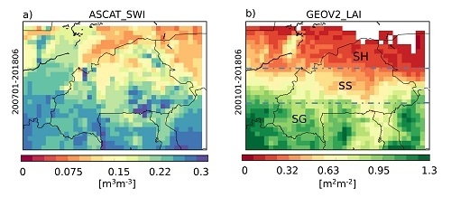
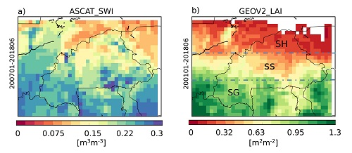
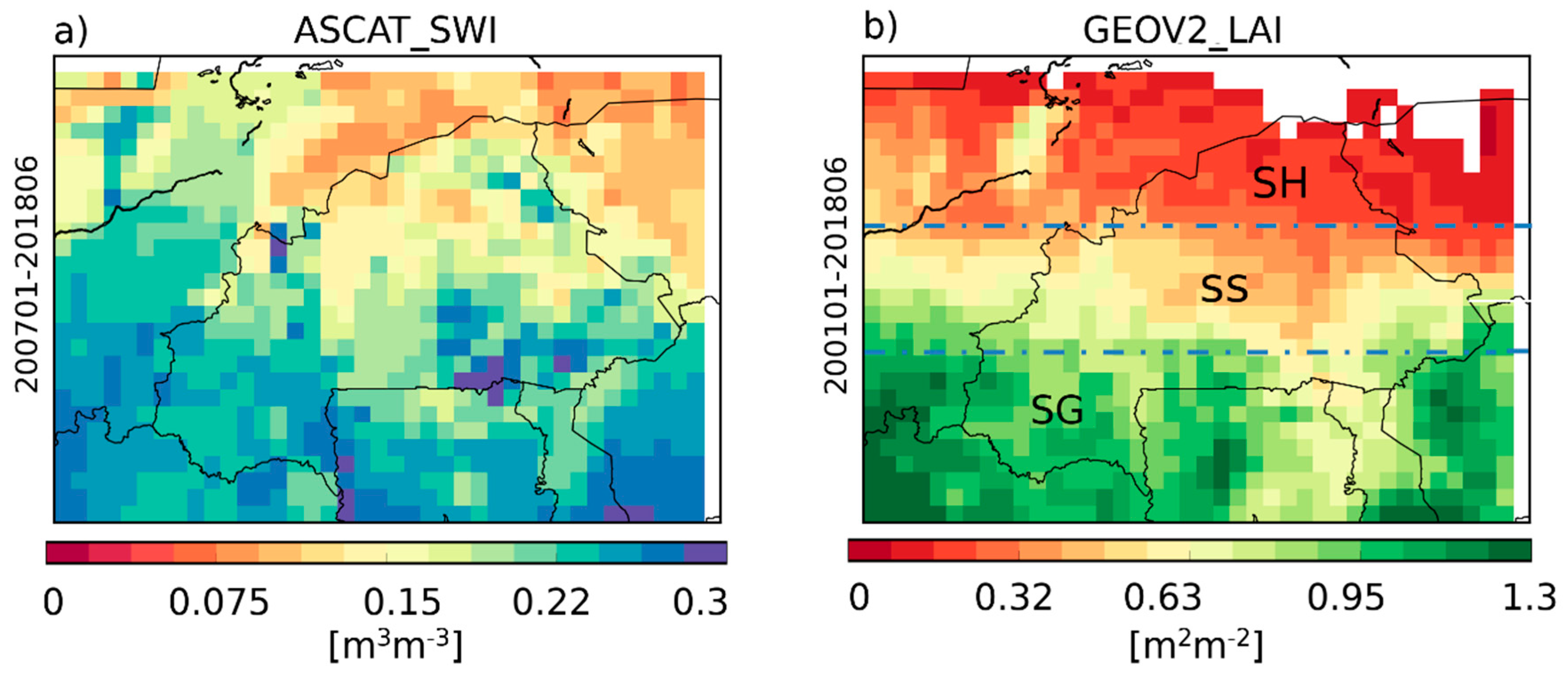
2.2.3. ASCAT Soil Water Index and GEOV2 Leaf Area Index

This study uses the ASCAT Soil Water Index (SWI) product distributed by the CGLS through its third version, i.e., SWI-001 Version 3.0. The SWI refers to the soil moisture content in relative units between 0 (dry) and 100 (saturated). It is computed based on a recursive exponential filtering method [52] using the backscatter observations from the ASCAT C-band radar on board MetOP satellites [53,54]. The SWI retrieved from the exponential filter using a T-value (characteristic time length; the higher the T-values, the smoother the SWI) of one day is used. It represents the SWI in the top soil layer [52]. It is used in the present study as a proxy for SSM. During the period considered in the experiment, the amount of soil moisture data increases in 2015 because the data from MetOP-B (launched in 2012) are used in addition to those from MetOP-A (launched in 2006) (see

Table 1. Yearly N points of SWI and LAI from 2007 to 2018–06.

	2007	2008	2009	2010	2011	2012	2013	2014	2015	2016	2017	2018
SWI	36,154	39,624	38,761	41,687	41,699	41,652	41,086	41,129	173,818	319,565	319,097	157,476
LAI	37,107	37,500	37,342	37,425	37,269	36,706	37,024	38,778	38,839	38,757	38,243	19,908

). Figure 1a presents the map of the average ASCAT SSM estimate for the whole January 2007–June 2018 period over the study area. For more details on the ASCAT SSM, readers are referred to [29]. Consistent with previous studies, e.g., [55], SSM displays a typical spatial structure, which is dominated by a strong meridional gradient (with wetter soil to the South and drier to the North). Some smaller scale patterns also emerge, such as enhanced SSM spots along the Sourou river (13.04°N, 3.04°W) and around Niono in Mali (around 14.15°N, 5.59°W) in the north eastern part of the domain. These are consistent with the existing mapping of water bodies in the region (e.g., [56]) and are also probably related to the presence of irrigated rice puddles and crops [57].

For the purpose of assimilating the SSM product, a rescaling of observations into model climatology space is needed in order to avoid introducing any artificial bias in the system caused, for example, by a possible mis-specification of physiographic parameters related to soil texture types [54,58]. To that end, the SWI product is transformed into model-equivalent SSM (from the model second layer of soil, 1–4 cm), based on the first two statistical moments (the mean and the variance) through a linear transformation [59]. The relevance of performing a seasonal rescaling was emphasized by several studies (e.g., [37,47]). In this study, the matching of SSM statistical distributions was made on a monthly basis by using a 3-month moving window over the January 2007–June 2018 period after screening for the presence of urban areas (>15%) and complex terrains (1500 m a.s.l.). Finally, the SWI observations are interpolated by an arithmetic average to the 0.25° model grid points (from their original 12.5 km spatial resolution).

The GEOV2 LAI observations are also distributed by the CGLS. They are retrieved from the SPOT-VGT and PROBA-V satellite data using the methodology prescribed in [60]. The 1 km × 1 km resolution observations are interpolated to 0.25° model grid points through an arithmetic average as in [19], so that at least 75% of the grid points are observed. In terms of temporal resolution, LAI observations are available with a 10-day frequency (at best). Figure 1b illustrates the averaged LAI (January 2001–June 2018). As in Figure 1a, the spatial structure of LAI is dominated by a strong meridional gradient (from lower LAI to the North to higher LAI to the South). This corresponds to three climatic regions: The Sahel (SH), the Sudan-Sahel (SS), and the Sudan-Guinea (SG). The country’s climate is characterized by two distinct seasons: A dry season and a rainy season (May to October) with growing seasons varying from six (SG region) to three (SH region) months [22]. Observations are rescaled to match the spatial resolution of the two atmospheric forcing data-sets, 0.25° × 0.25° and 0.50° × 0.50° for ERA5 and ERA-Interim, respectively

2.2.4. Evapotranspiration, Gross Primary Production, and Sun-Induced Fluorescence

Independent datasets of evapotranspiration and gross primary production (GPP) are used to assess the quality of the LDAS-Monde reanalysis of LSVs.

Terrestrial evapotranspiration estimates are from the GLEAM (Global Land Evaporation Amsterdam Model) v3.1. product [61]. They cover the period of 1980–2016 and are available at a spatial resolution of 0.25° × 0.25°. The GLEAM dataset is widely used for investigating both trend and spatial variability in the terrestrial water cycle (e.g., [62,63,64]) as well as land atmosphere interactions (e.g., [65,66]). In short, the model computes the terrestrial evaporation and root-zone soil moisture [55] and is mainly driven by microwave remote sensing observations, the potential evaporation amount being constrained by satellite-derived soil moisture.

For the evaluation of GPP, we use estimates derived from meteorological parameters through the use of machine learning algorithms within the FLUXCOM project [67]. This set of observations can be found at the Max Planck Institute for Biogeo-chemistry data portal (https://www.bgc-jena.mpg.de/geodb/projects/Home.php, last access: November 2018) and is available at a 0.5° x 0.5° spatial resolution with a monthly temporal frequency over the 1982-2013 period. In this study, GPP products were used over the 2001–2013 time period.

We also use estimates of sun-induced fluorescence (SIF) from the GOME-2 (Global Ozone Monitoring Experiment-2) scanning spectrometer [68,69] to evaluate GPP. Leroux et al. [43] has shown that observations of SIF can be used as a proxy to evaluate the influence of data assimilation on simulated GPP using correlations. We use in this study the Level-3 v27 SIF product, giving a daily-averaged SIF at 0.5° × 0.5° resolution over the 2010–2016 period.

Observations are rescaled to match the spatial resolution of the two atmospheric forcing data-sets, 0.25° × 0.25° and 0.50° × 0.50° for ERA5 and ERA-Interim, respectively.

2.3. Experimental Setup and Evaluation Strategies

In this study, we first evaluate both precipitation and SW_in variables from ERA-Interim and ERA5 reanalyses against in situ measurements. Then, LDAS-Monde is driven by both ERA5 and ERA-Interim reanalyses, with all atmospheric variables interpolated at a spatial resolution of 0.25° × 0.25° and 0.5° × 0.5°, respectively. In order to drive the model to the equilibrium state, the first year (2001) is spun-up 20 times for both the ERA5 (LDAS-ERA5 hereafter) and ERA-Interim (LDAS-ERAI hereafter) configurations. Then, a comprehensive application of LDAS-Monde is performed using the SEKF as well as its open-loop counterpart (model only without assimilation). It is the same framework as used in [19]. The experiment covers the period of 2001–June 2018.

Performance metrics are used (i) to assess the ability of LDAS-Monde to represent the land surface conditions as well as (ii) to evaluate ERA-Interim and ERA5 reanalyses. Metrics, such as the correlation coefficient (R), mean bias, standard deviation of differences (SDD), root mean squared differences (RMSD), unbiased RMSD (ubRMSD), and bias, are applied. A 10,000 samples bootstrapping is used to determine the 95% confidence interval of the median from the precipitation reanalyses (see

Table 2. Comparison of precipitation and incoming solar radiation forcing with in situ observations for ERA5 and ERA-Interim over the period of 2010–2016 (based on monthly sum). Scores are given for significant correlations with p-values < 0.05.

	Median R 1, 95% Confidence Interval 2 (% of Stations for Which This Configuration Is the Best)	Median ubRMSD 1 on Precipitation Time Series (in mm/month) and Incoming Solar Radiation (in w·m−2), 95% Confidence Interval 2 (% of Stations for Which This Configuration is the Best)	Median Bias 1 on Precipitation Time Series (in mm/month) and Incoming Solar Radiation (in w·m−2), 95% Confidence Interval 2 (% of Stations for Which This Configuration is Better)	Median RMSD 1 on Precipitation Time Series (in mm/month) and Incoming Solar Radiation (in w·m−2), 95% Confidence Interval 2 (% of Stations for Which This Configuration is Better)
ERA5 (precipitation)	0.82 ± 0.009 (84%)	52.02 ± 1.39 (89%)	−15.00 ± 3.27 (83%)	56.15 ± 3.60 (86%)
ERA-Interim (precipitation)	0.77 ± 0.010 (16%)	58.44 ± 1.42 (11%)	−19.85 ± 3.77 (17%)	63.89 ± 3.25 (14%)
ERA5 (incoming solar radiation)	0.59 ± 0.07 (100%)	36.23 ± 6.48 (100%)	19.40 ± 32.43 (100%)	42.24 ± 21.76 (100%)
ERAI (incoming solar radiation)	0.46 ± 0.15 (0%)	41.03 ± 4.22 (0%)	28.12 ± 29.80 (0%)	50.72 ± 18.63 (0%)

¹ Only for stations presenting significant R values on precipitation time series (p-value < 0.05): 134 stations; ² 95% confidence interval of the median derived from a 10,000 sample bootstrapping.

). For the evaluation of both precipitation and SW_in from ERA5 and ERA-Interim reanalyses, the 2010–2016 period and the year of 2017 are considered, respectively.

3. Results

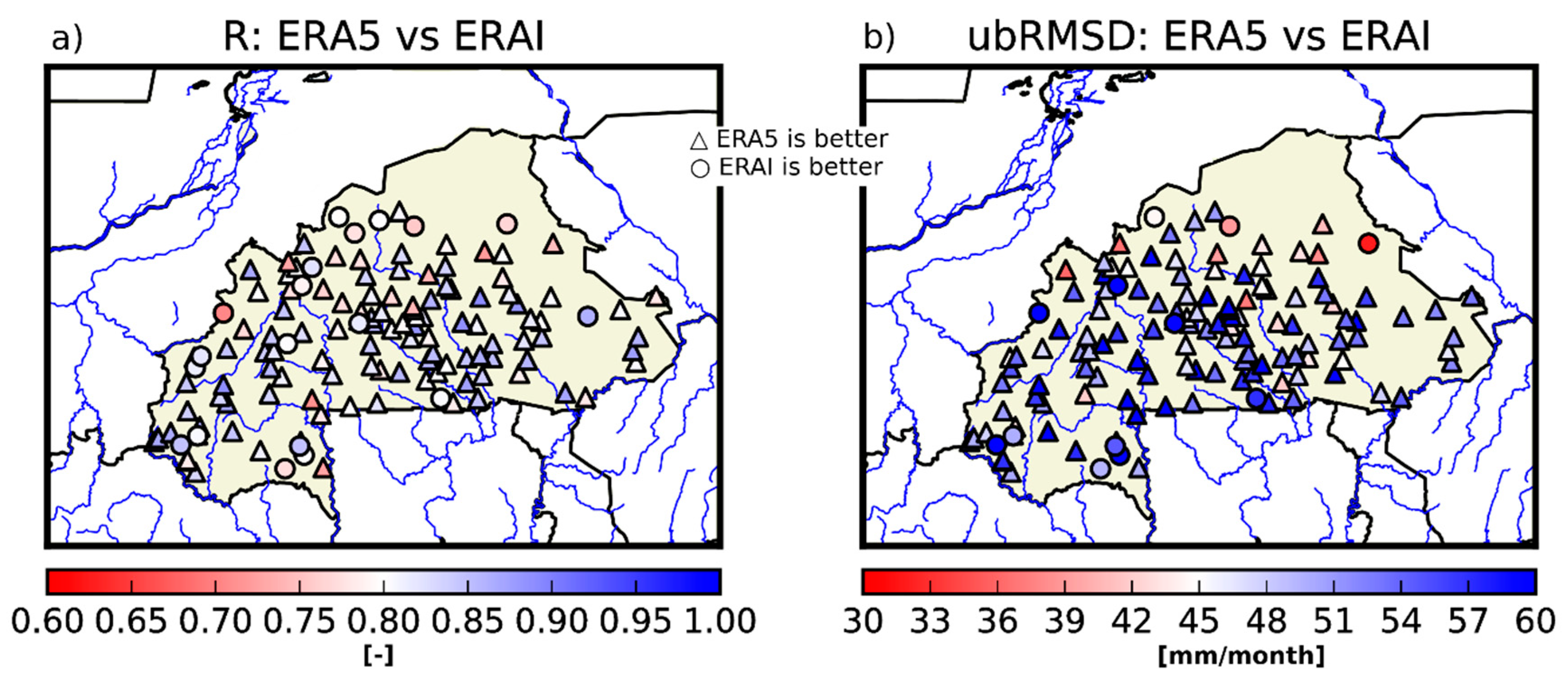
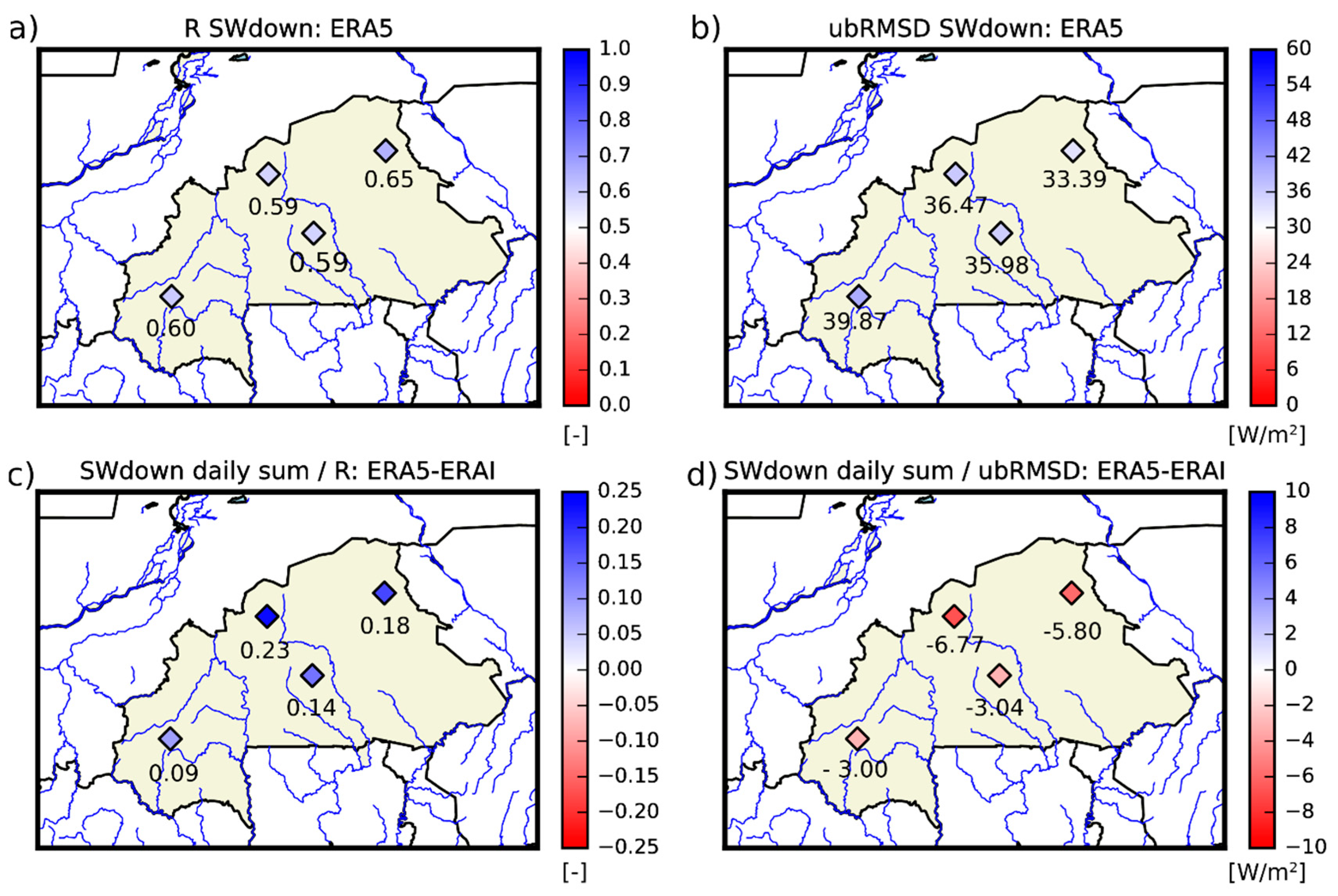
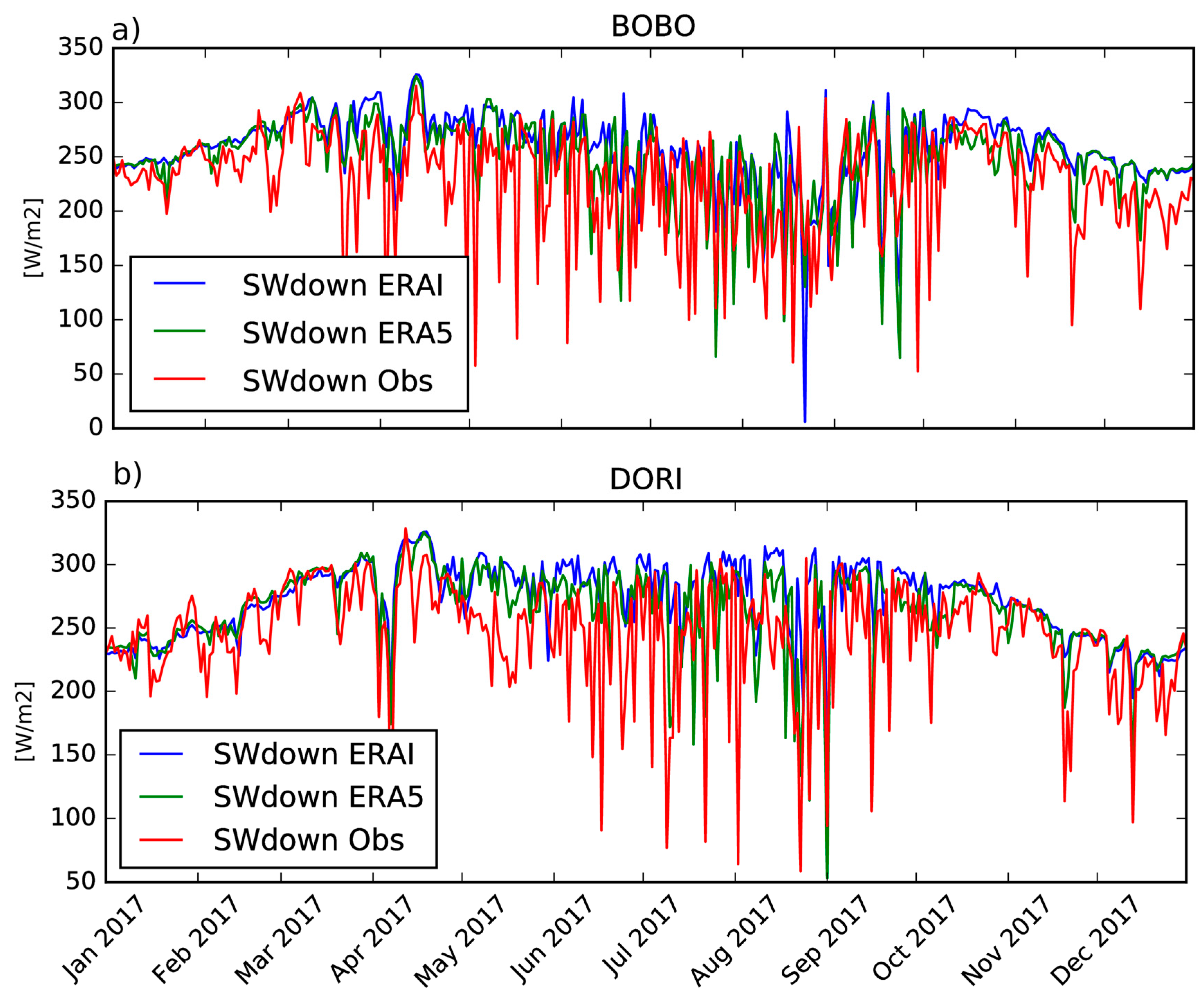
3.1. Evaluation of ERA5 and ERA-Interim Reanalyses

The performance of ERA5 and ERA-Interim precipitation and SW_in is assessed by comparing reanalyses with the in situ measurements described earlier.

The statistical scores for 2010–2016 daily precipitation from ERA5 and ERA-Interim with respect to 134 gauge stations spanning all over BF are shown in Table 2. The Median R, ubRMSD, bias, and RMSD values for the total monthly precipitation time series along with their 95% confidence interval are 0.82 ± 0.009, 52.02 ± 1.39 mm/month, −15.00 ± 3.27 mm/month, and 56.15 ± 3.60 mm/month for ERA5, and 0.77 ± 0.010, 58.44 ± 1.42 mm/month, −19.85 ± 3.77 mm/month, and 63.89 ± 3.25 mm/month for ERA-Interim. These results demonstrate the ability of ERA5 reanalysis to better represent precipitation variability than ERA-Interim. ERA5 performs better than ERA-Interim for 84% of the precipitation gauging stations for R values, 89% for ubRMSD values, 83% for bias values, and 86% for RMSD values. This is also illustrated by the maps in Figure 3, where triangle (circle) symbols indicate stations where ERA5 performs better (worse) than ERA-Interim in terms of R (Figure 3a) and ubRMSD (Figure 2b). Overall, triangle symbols dominate the two maps of Figure 3, which implies that ERA5 precipitation reanalyses are in better agreement with in situ observations than ERA-Interim over BF. Precipitation from ERA-interim or ERA5 are both closer to in situ observations in the northern (lower ubRMSD values) than in the southern part of the domain. Overall, ERA5 performs better than ERA-Interim, likely due to an improved representation of convective precipitation in the tropical region [70] and to the larger number of assimilated data; it is also possibly related to its higher spatial resolution.

The statistical scores for the 2010–2016 daily mean surface SWin from ERA5 and ERA-Interim with respect to four stations (see Figure 4) are shown in Table 2. Median R, ubRMSD, bias, and RMSD values along with their 95% confidence interval are 0.59 ± 0.07, 36.23 ± 6.48 W/m², 19.40 ± 32.43 W/m², and 42.24 ± 21.76 W/m² for ERA5, and 0.46 ± 0.15, 41.03 ± 4.22 W/m², 28.12 ± 29.80 W/m², and 50.72 ± 18.63 W/m² for ERA-Interim.

Figure 4 shows maps of R and ubRMSD values between ERA5 daily mean surface SW_in and in situ measurements at four stations (Figure 4a,b) as well as their differences against R and ubRMSD values from ERA-Interim (Figure 4c,d) over 2017. From Figure 4, one can clearly observe higher correlations and lower ubRMSD values for ERA5 compared to ERA-Interim for the considered four stations. This is consistent with the observed positive correlation differences (ERA5—ERA-Interim, Figure 4c) and negative ubRMSD differences (ERA5—ERA-Interim, Figure 4d). Figure 4 shows the 2017 time series of the daily SW_in for ERA-Interim (blue), ERA5 (green), and the in situ observations (red) for Bobo (Figure 5a; 11.16°N, 4.30°W) and Dori (Figure 5b; 14.03°N, 0.03°W) stations belonging to the SG and SS zones, respectively. At these subtropical sites, the temporal structure of the annual cycle of SW_in is strongly shaped by the top-of-the atmosphere incoming radiation, which drives the two well defined maxima of SW_in [71,72]. At Bobo, they occur in April and October while further North in Dori, the second maximum is less pronounced. Both reanalyses broadly capture these features, even though they tend to overestimate SW_in (in particular during the monsoon, when clouds induce sharp drops which can reach more than 100 W/m²)—a similar bias also noted by [73] at the relatively close Sahelian site of Niamey. However, this bias is slightly reduced in ERA5. This implies that ERA5 performs better in representing SW_in variations than ERA-Interim over BF. This better performance of ERA5 is also probably related to the implementation of an improved radiation scheme (see [74] for more details).

3.2. LDAS-Monde Impact

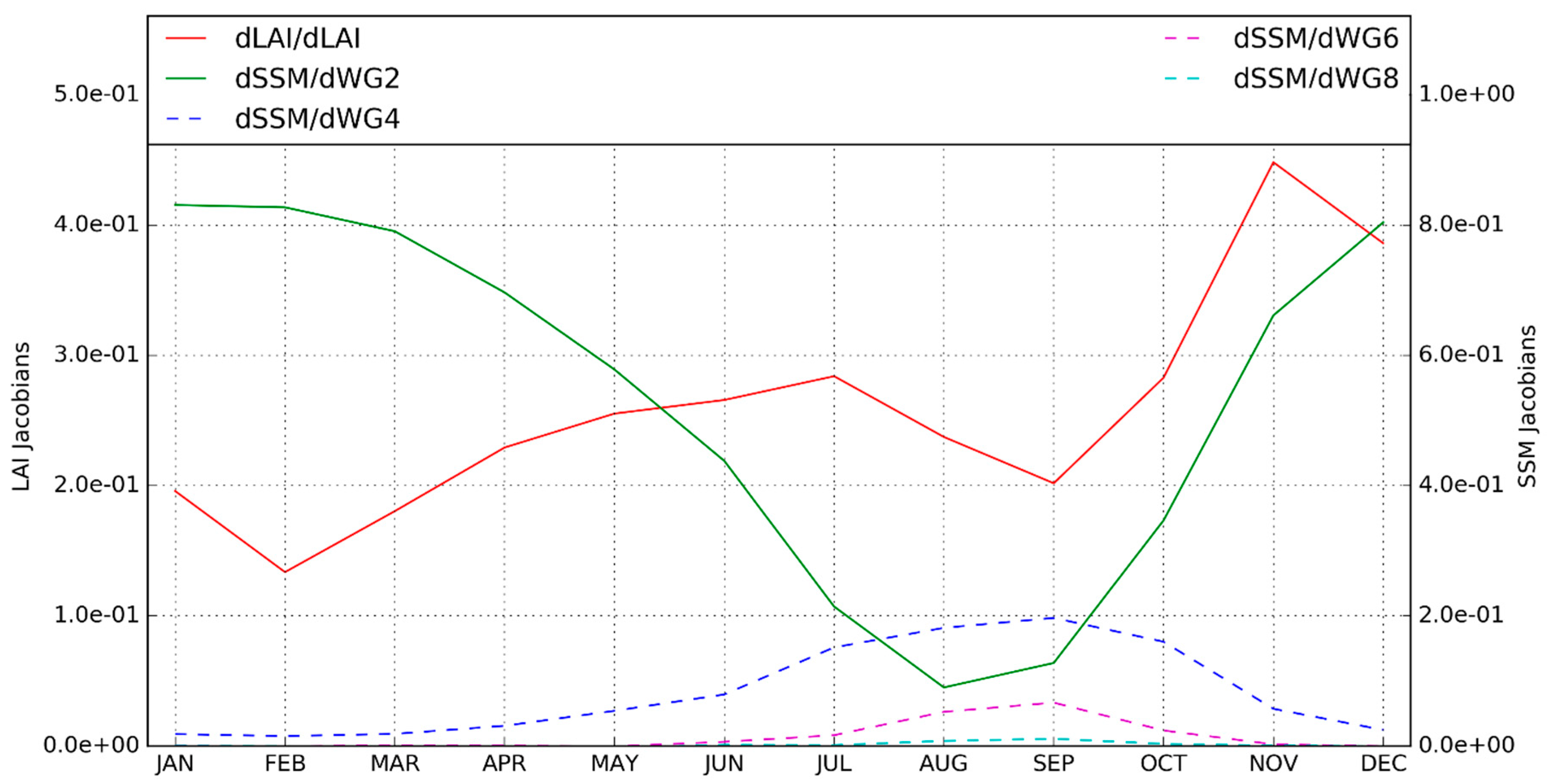
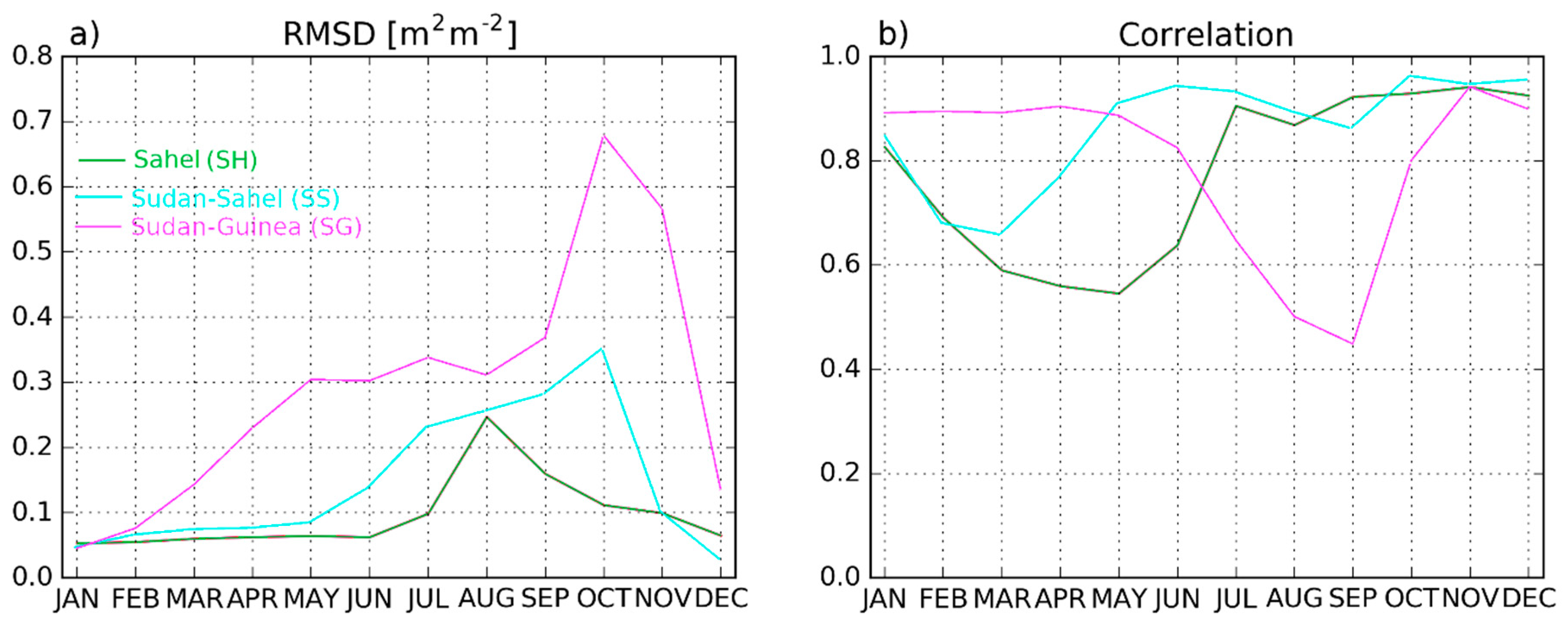
3.2.1. Model Sensitivity to the Observations

The Jacobians are governed by the physics of the model and their examination is crucial to understand the data assimilation system performances [19,40,41,75]. Mean Jacobians values over January 2010 to June 2018 for the whole domain of Burkina-Faso are presented in

Table 3. Mean Jacobians values for the eight control variables considered in this study over the whole spatial domain for January 2001 to June 2018.

January 2001 to June 2018		$\frac{\delta SSM}{\delta LAI}$ 1–4 cm	$\frac{\delta SSM}{\delta w_3}$ 4–10 cm	$\frac{\delta SSM}{\delta w_4}$ 10–20 cm	$\frac{\delta SSM}{\delta w_5}$ 20–40 cm	$\frac{\delta SSM}{\delta w_6}$ 40–60 cm	$\frac{\delta SSM}{\delta w_7}$ 60–80 cm	$\frac{\delta SSM}{\delta w_8}$ 80–100 cm
Mean	–0.0006	0.5372	0.2033	0.0818	0.0441	0.0142	0.0049	0.0020
	$\frac{\delta LAI}{\delta LAI}$	$\frac{\delta LAI}{\delta w_2}$ 1–4 cm	$\frac{\delta LAI}{\delta w_3}$ 4–10 cm	$\frac{\delta LAI}{\delta w_4}$ 10–20 cm	$\frac{\delta LAI}{\delta w_5}$ 20–40 cm	$\frac{\delta LAI}{\delta w_6}$ 40–60 cm	$\frac{\delta LAI}{\delta w_7}$ 60–80 cm	$\frac{\delta LAI}{\delta w_8}$ 80–100 cm
Mean	0.2578	0.0134	0.0223	0.0432	0.0911	0.0522	0.0318	0.0188

.

The top row of Table 3 represents the impact of perturbating individually each control variable of LDAS-Monde (LAI, soil moisture from layers 2 to 8), by a (positive) small amount at the beginning of an assimilation window, on the model equivalent of SSM at the end of the assimilation window (i.e., 24 hours later). As the model equivalent of SSM is the second layer of soil (W₂ between 1 and 4 cm depth), it is expected that the sensitivity of SSM to changes in soil moisture of that layer ($\frac{\delta SSM}{\delta w_2}$) will be higher compared to those of the other layers of soil ($\frac{\delta SSM}{\delta w_3}$ to $\frac{\delta SSM}{\delta w_8}$). As seen in Table 3, the mean Jacobian value is clearly higher for W₂ than for any other layers. The model sensitivity to SSM decreases with depth, suggesting that the assimilation of SSM will be more effective in modifying soil moisture from the first layers than the deeper layers. Over Burkina-Faso, mean Jacobian values with respect to SSM observations (Table 3, top rows) range from 0.5372 to 0.0020 for layers, w₂ to w₈, respectively and is –0.0006 for LAI ($\frac{\delta SSM}{\delta LAI}$). This negative value indicates that a small positive increments of LAI will generally lead to a decrease of SSM (w₂).

Table 3, bottom row, shows the same for LAI: The sensitivity of LAI to changes in LAI ($\frac{\delta LAI}{\delta LAI}$) and in soil moisture ($\frac{\delta LAI}{\delta w_2}$ to $\frac{\delta LAI}{\delta w_8}$), from left to right, respectively. The sensitivity of LAI and in soil moisture suggests that the control variables related to soil moisture will also be impacted by the assimilation of LAI. Table 3 also illustrates that the assimilation of LAI will be more effective in modifying soil moisture from layers 4 to 6 than from the surface layers.

Figure 6 illustrates the seasonal cycles of the Jacobians averaged over January 2001 to June 2018. For sake of clarity, only $\frac{\delta LAI}{\delta LAI}$,$\frac{\delta SSM}{\delta LAI}$,$\frac{\delta SSM}{\delta w_4}$,$\frac{\delta SSM}{\delta w_6}$, and $\frac{\delta SSM}{\delta w_8}$ are presented. Looking at the SSM Jacobians, the depth impact already highlighted by Table 3 is visible (i.e., less sensitivity to surface soil moisture at deeper layers than at upper layers). From Figure 6, a seasonal impact is also visible, $\frac{\delta SSM}{\delta LAI}$ are higher in winter months than in summer months, suggesting that LDAS-Monde will be more efficient at assimilating SSM during winter months. Similarly, from $\frac{\delta LAI}{\delta LAI}$, one may notice a dual seasonal cycle; LDAS-Monde will be more efficient at assimilating LAI during April to June, and October to November.

It is worth mentioning that the configuration where ERA5 is used to force LDAS-Monde was considered to present the Jacobians evaluation. Using the ERA-Interim configuration leads to similar results (not shown).

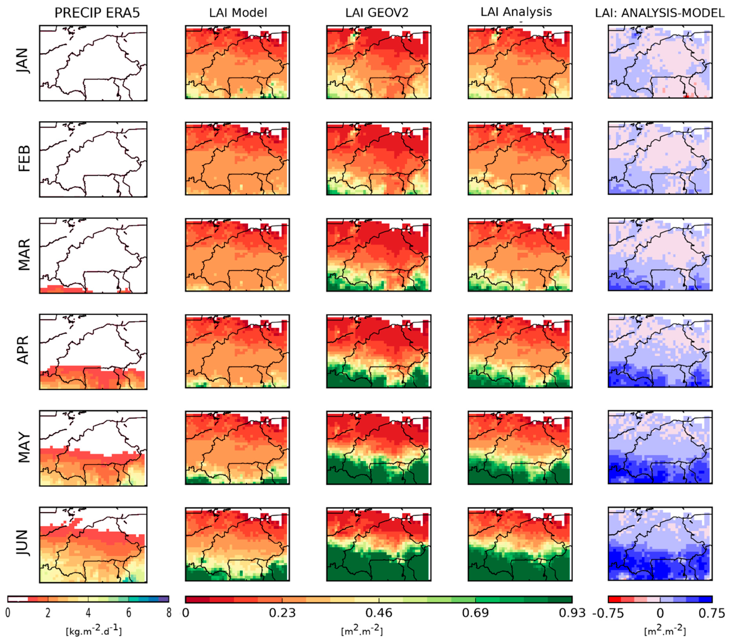
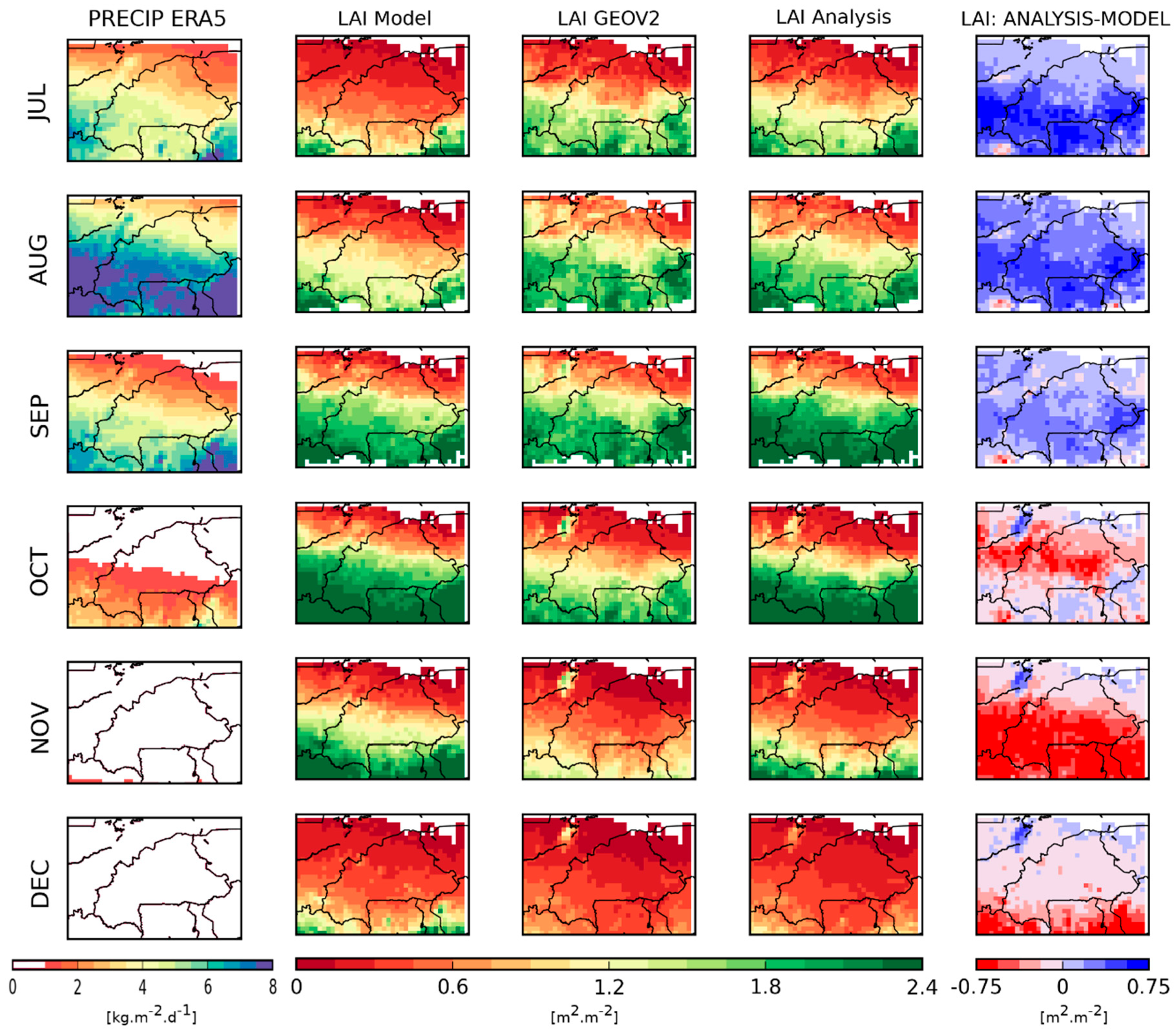
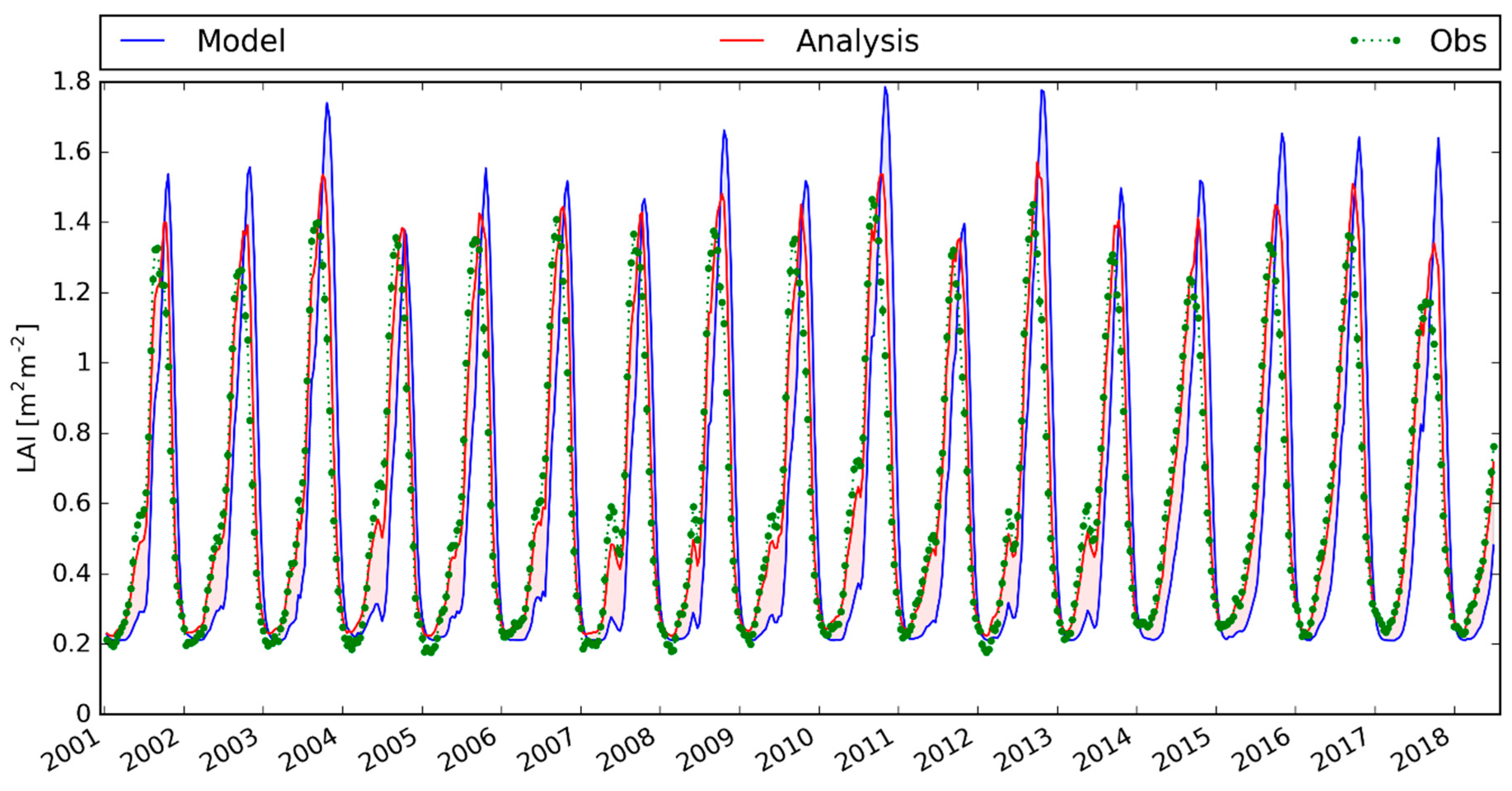
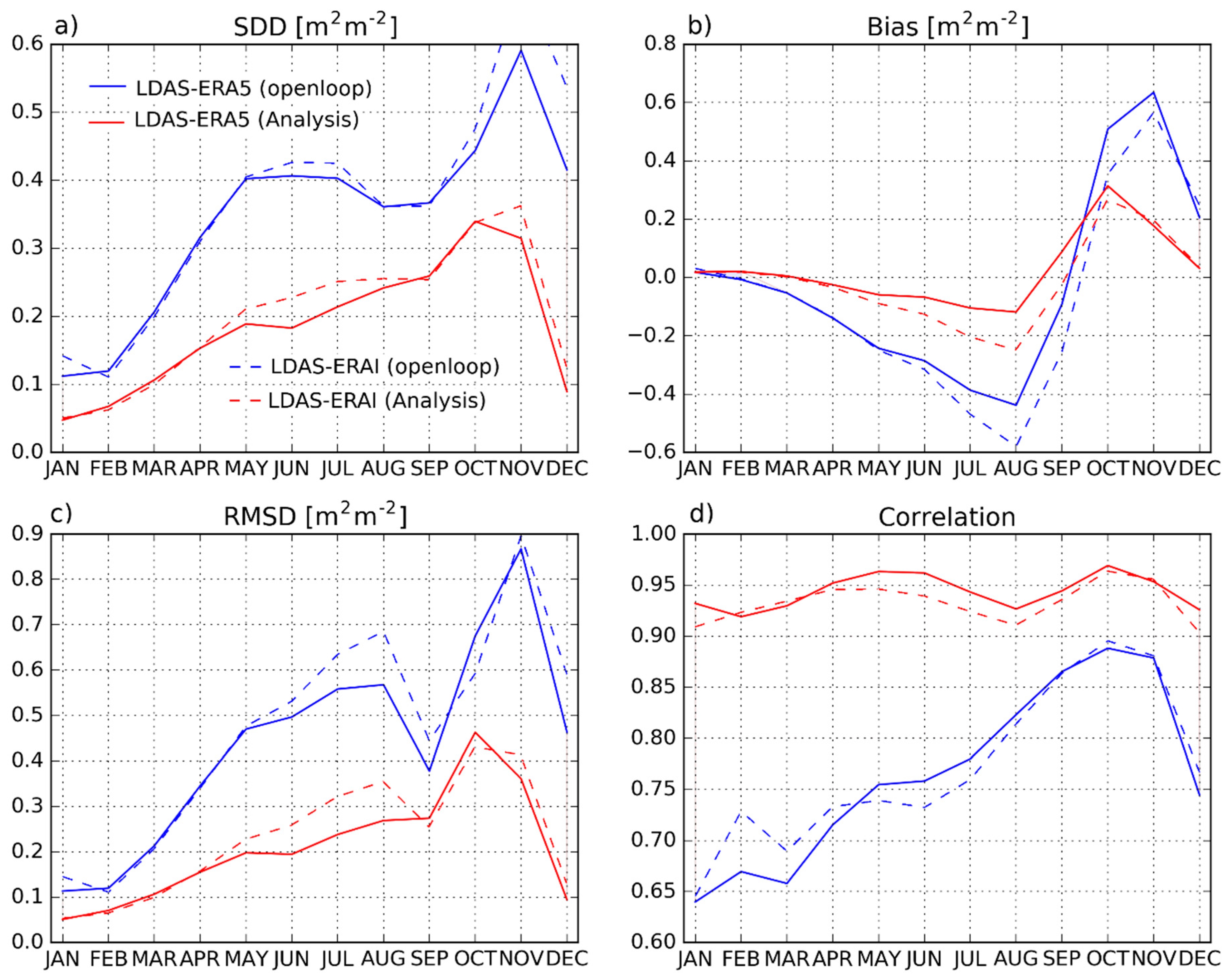
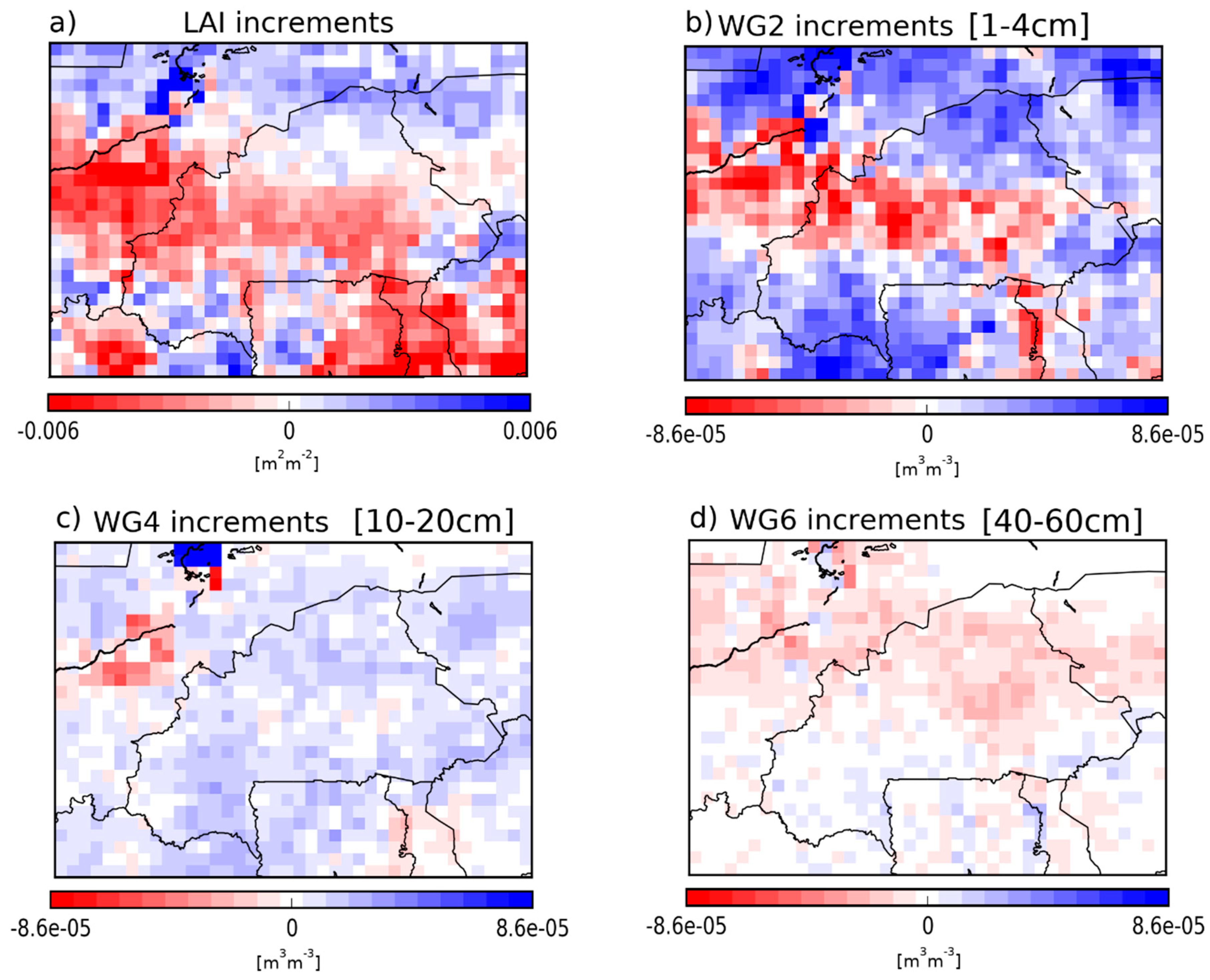
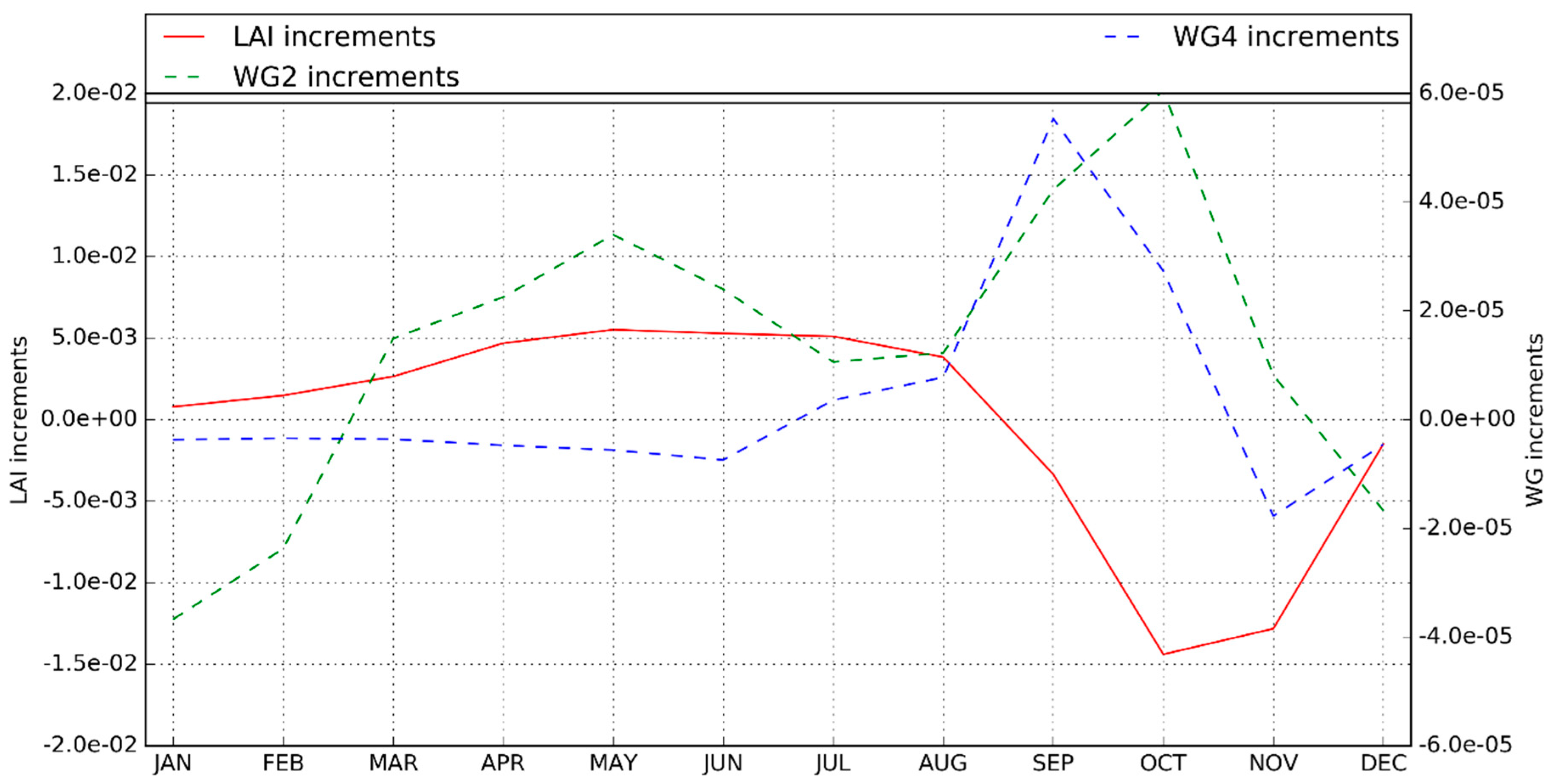
3.2.2. Assimilation Impact on LAI and Soil Moisture

In order to obtain the land surface analysis, satellite derived observations are combined with the model simulations through the above-mentioned data assimilation technique. In doing that, the resulting analysis is expected to be closer to the assimilated observations (LAI and SSM) than the open-loop (i.e., model with no assimilation). The largest impact is observed for LAI. Figure 7 shows maps of the monthly average values of precipitation from ERA5 as well as LAI from the LDAS-ERA5 openloop, the observations, LDAS-ERA5 analysis, and the difference between the analysis and the openloop. Observations indicate a sharp jump of LAI in April, very likely in response to the increase of soil moisture availability due to the start of the rainy season. However, an increase in LAI is also observed earlier in the SG region (southern part of the domain) from February to May; i.e., before the first rains. Interestingly, this peculiar behaviour would be consistent with findings from in situ studies from [76,77,78], which point to some tree species that put on leaves before the first rains of the season. This functioning does not appear to be linked to soil moisture [79]. It could involve rises of the air temperature or humidity, though the precise mechanisms at play are still unknown. In any case, this process is not represented in the ISBA LSM, leading to a temporal shift of two to three months in the leaf onset and an underestimation of the observed LAI.

Figure 7 also shows little impact of the assimilation on the estimated LAI where observations are below 0.4 m²·m⁻². This is due to a limitation of the ISBA LSM. As mentioned in Section 2.1.1, a minimum LAI threshold is prescribed to 0.3 m²·m⁻² for every vegetation type (except coniferous forests) in ISBA. To satisfy that threshold, we force the SEKF to reset every LAI estimate below 0.3 m²·m⁻² to that value, thus limiting the impact of assimilation.

Figure 8 presents similar maps for the following months, from July to December. While the model underestimates LAI in spring, it significantly overestimates the LAI in November, after the demise of the rainy season.

The analysis is efficient at compensating for these two model caveats, as shown in Figure 7 and Figure 8. This is also clear in Figure 9, which shows the LDAS-ERA5 configuration LAI monthly mean time series averaged values over the whole domain for January 2001 to June 2018. Observations indicate interannual fluctuations in the yearly maximum of LAI, with, for instance, higher values in 2003, 2010, and 2012 and lower values in 2002, 2011, and 2017 (consistent with [80,81]). Beyond differences in the structure of their annual cycles, the model and the analysis both capture part of this interannual variability.

The improved annual cycle of LAI provided by the analysis is associated with a higher correlation and a positive impact on the SDD, Bias, and RMSD scores over the study region in all months (as seen on Figure 10). It is also visible that the analyses add skill to both configurations, LDAS-ERA5 and LDAS-ERAI, which indicates the healthy behavior from the land data assimilation system.

Considering now the three climatic regions of BF, it appears that the correlation between the analyzed and observed LAI is lower during the rainy season in the SG region while it is higher in the SS and SH regions (Figure 11b for the LDAS-ERA5 configuration). This reduction of R values in the analysis during the rainy season in the SG region could be related to a decrease in the number of the observed LAI linked to cloud cover (see

Table 4. Seasonal number of LAI values (N) from 1 January 2001 to 30 June 2018 for the LDAS-ERA5 configuration.

	Jan.	Feb.	Mar.	Apr.	May	Jun.	Jul.	Aug.	Sep.	Oct.	Nov.	Dec.
BF	59,724	59,723	59,724	59,715	58,914	53,840	48,140	48,006	46,022	54,265	56,406	56,406
SH	18,684	18,683	18,684	18,679	18,674	18,678	17,638	17,644	17,646	17,646	17,646	17,646
SS	19,440	19,440	19,440	19,440	19,440	19,440	18,334	18,357	18,319	18,360	18,360	18,360
SD	21,600	21,600	21,600	21,596	20,800	15,722	12,168	12,005	10,057	18,259	20,400	20,400

). Overall, the assimilation corrects the model seasonal responses by increasing the LAI during the rainy season and decreasing the LAI after the rainy season, especially in the Sudanian region (SS and SG regions).

Analysis increments for the LAI and for soil moisture from the LDAS-ERA5 configuration in (i) the second layer of soil (w₂, between 1 and 4 cm), (ii) the fourth layer (w₄, between 10 and 20 cm), and (iii) the sixth layer (w₆, between 40 and 60 cm) are averaged for the period of January 2001 to June 2018. They are presented in Figure 12. Overall, the analysis removes the LAI in the central part (SS) of the domain. However, small spots of increases are noticeable in both the south-western (SG) and north-eastern part (SS) of the domain. Regarding the w₂ soil moisture values, the analysis adds water in some parts of the domain (SH, SG, and the eastern part of SS) and removes water in the central part. For w₄ and w₆, i.e., for deeper soil layers, the impact is less pronounced (in agreement with the above mentioned study of the Jacobians), but a perceptible north-eastward oriented drying is still observed. It is worth mentioning that the dark blue point in the north-western part of Figure 12a (positive LAI increments) around Mopti in Mali corresponds to the Niger inner delta, including wetlands and irrigated areas. Irrigation is not accounted for in the version of ISBA used in this study and the analysis tends to compensate for this model weakness. This area is also visible in the map of the observed LAI (Figure 1b). While Figure 12 illustrates analysis increments for the LDAS-ERA5 configuration, the LDAS-ERAI one follows the same description (not shown).

As mentioned above, the impact of assimilation on SSM is relatively weaker than on LAI. This can be seen, for instance, in Figure 13a, which shows the correlation values between SSM from the openloop and the analysis (for both LDAS-ERA5 and LDAS-ERAI configurations) and the SSM estimates from CGLS. Note that the seasonality effect has been removed through the use of the anomaly time series in order to assess the shorter-term variability of soil moisture. Figure 13a indicates a positive impact of the assimilation especially from January to May and from October to December regarding the model, emphasizing the improvement in SSM values. The impact of the assimilation on the representation of the shorter-term soil moisture variability is further presented using maps of the anomaly correlations between soil moisture before and after assimilation against ASCAT SSM estimates (Figure 13b,c); as well as using their correlation differences (Figure 13d) for the LDAS-ERA5 configuration. It is evident from Figure 13b,c that the analysis improves soil moisture simulations over the whole domain with a more pronounced impact over the Sudanian region, i.e., SH and SG (Figure 13c). Looking at the correlation differences based on the anomaly time series (Figure 13d), it is evident that positive values dominate, especially in the SH and SS regions, along with a rather neutral effect in the southern part of the domain.

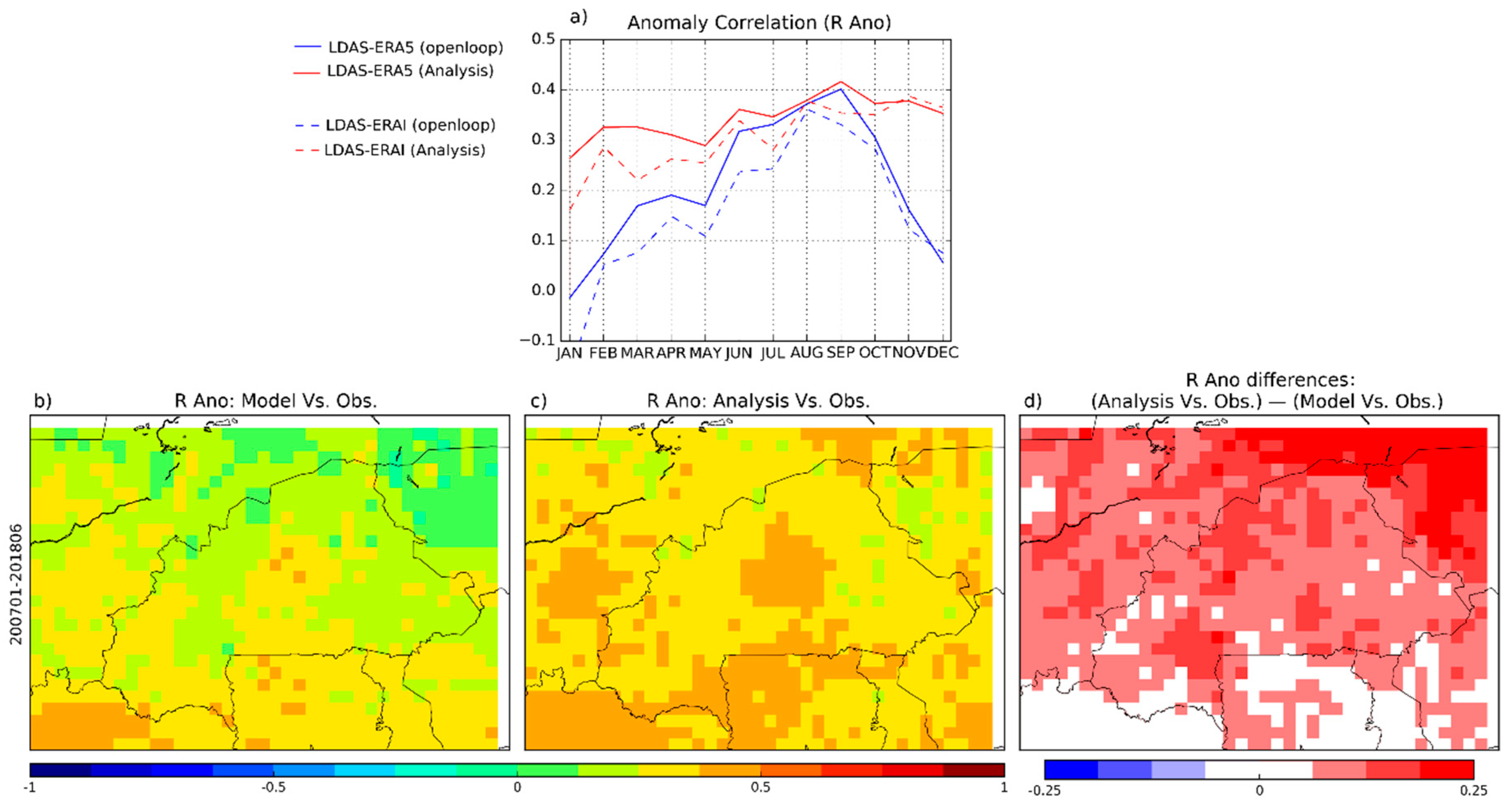
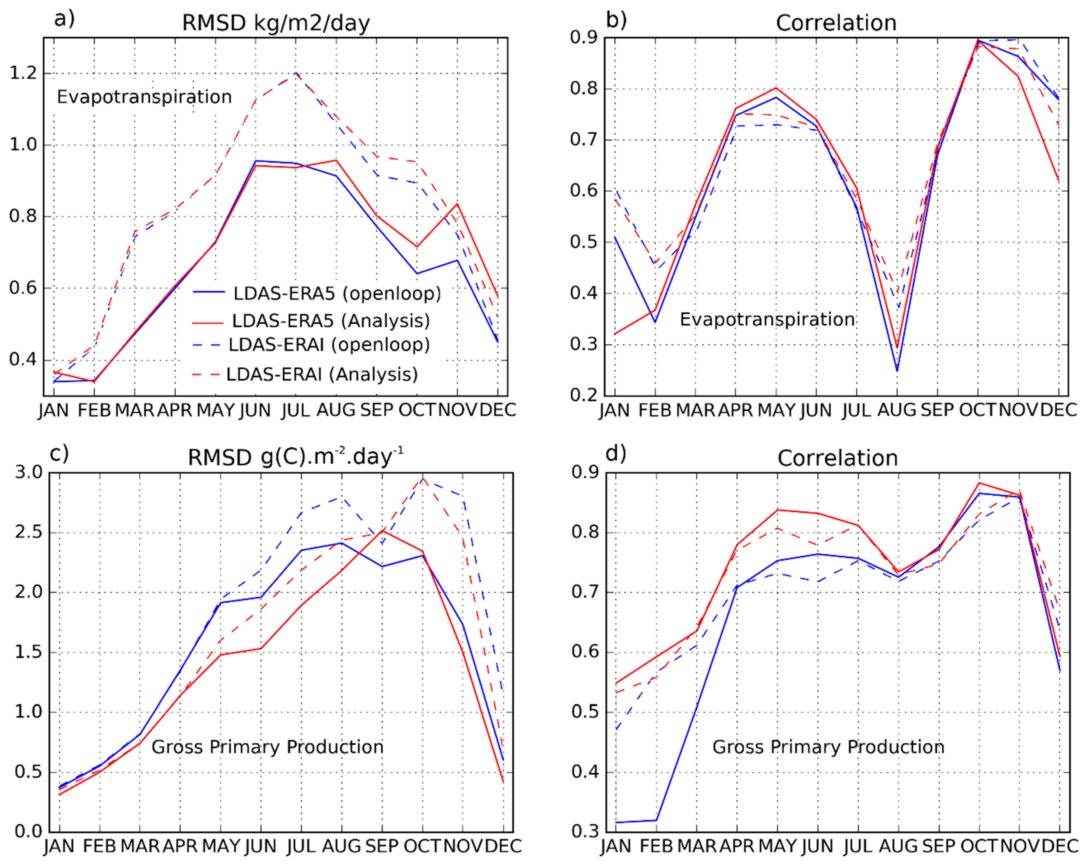
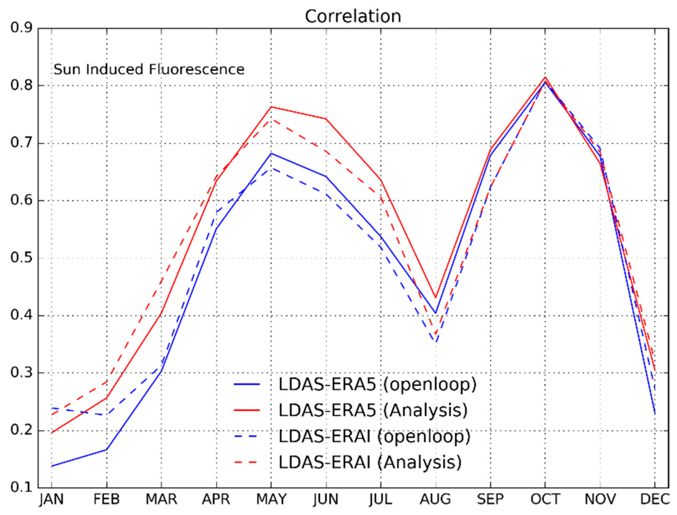
3.2.3. Evaluation Using Independent Datasets

For evapotranspiration and GPP, seasonal scores (RMSD and R values in Figure 14) are computed for the model and for the analysis in both the LDAS-ERA5 and LDAS-ERAI configurations. Only vegetated grid points (>90%) are considered. After the joint assimilation of SSM and LAI, a small positive impact on evapotranspiration is observed for the correlations, as found in [40], and it is interesting to note a small degradation of the RMSD values in the second part of the year (August to December). However, there is a clear improvement in GPP in terms of the RMSD and R scores, especially from January to August (Figure 14c,d). While the impact on R values of the analysis is equally distributed over the domain for both evapotranspiration and GPP, a larger (positive) impact on RMSD values is found on the southern part of the domain (not shown). This is in agreement with the analysis impact on LAI described above. LDAS-ERA5 generally performs better than LDAS-ERAI for both the openloop and the analysis. It is particularly true when considering RMSD values for evapotranspiration (Figure 14a).

Figure 14a indicates, however, the degradation of the evapotranspitation estimation by LDAS-ERA5 and LDAS-ERAI when compared to the GLEAM dataset. It is worth noting that the GLEAM dataset is not a direct remotely sensed observation, but rather a remote sensing-based evaporation retrieved model with its own uncertainties. For instance, Pagán et al. (2018) [82] have recently assessed the potential of satellite observations of solar-induced chlorophyll fluorescence (SIF), normalized by photosynthetically-active radiation (PAR), to diagnose the ratio of transpiration to potential evaporation (“transpiration efficiency”) from several state of the art models, including SURFEX and GLEAM. They obtained better results with SURFEX than with GLEAM, in particular during the vegetation decaying phase.

Looking at the seasonal time series of the analysis increments (Figure 15 for the LDAS-ERA5 configuration), it is very interesting to notice that the degradation from the analysis over the open-loop (from August in both the LDAS-ERA5 and LDAS-ERAI configuration) corresponds to a sign inversion in the LAI increments (from positive to negative) as well as a sharp positive increase in soil moisture increments (analysis increments of soil moisture from the second (WG2) and fourth (WG4) layer of soil are presented). This situation in the vegetation decaying period seems conflictual and may suggest a lack of consistency between the two observation types (LAI and SSM), leading to the observed degradation in RMSD values.

For SIF, seasonal scores (R values in Figure 16) comparing the observed SIF and simulated GPP for vegetated grid points are computed for model and analysis estimates in both the LDAS-ERA5 and LDAS-ERAI configurations. A positive impact of DA on R can be seen from January to August with an averaged improvement of 0.1 on R for both configurations. For the rest of the year, the impact is rather neutral. Using ERA5 or ERA-Interim as atmospheric forcing does not have much influence on R. This was also the case for FLUXCOM GPP in Figure 14. This is due to a diminished impact of atmospheric forcing on the modelled GPP. The positive impact is of the same scale for the three agroclimatic areas covering BF (not shown). This is consistent with what was observed for correlations between simulated GPP and the FLUXCOM dataset.

4. Discussion and Conclusions

This study focused on the capability of LDAS-Monde to provide an improved reanalysis of land surface conditions through the joint assimilation of satellite-derived soil moisture and vegetation products over Burkina-Faso in western Africa. The LDAS-Monde offline system was forced by both ERA5 new atmospheric reanalysis and ERA-Interim former atmospheric reanalysis, leading to a 0.25° × 0.25° and a 0.5° × 0.5° degree spatial resolution reanalyses. The quality of ERA5 with respect to the former ERA-Interim reanalysis was evaluated using (i) in situ measurements of precipitation and incoming solar radiation (Sw_in) as well as (ii) the output of LDAS-Monde. The comparison of the two atmospheric forcing yields two key results: ERA5 provides substantial improvements compared to ERA-interim for precipitation (over 2010–2016), and also for the SW_in variable (over 2017). Using ERA5 and ERA-Interim to force the ISBA LSM (open-loop) provides a good model first guess, e.g., on the LAI variable with an advantage to ERA5. However, comparing the open-loop with the observed LAI has highlighted the missing processes in the representation of vegetation phenology. The assimilation is able to improve the simulation of both SSM and LAI when using either ERA5 or ERA-Interim, showing that the analyses add skill to both configurations and indicating the healthy behavior of LDAS-Monde. From the analysis, important improvements in the representation of the LAI, SWI, and GPP variables were obtained with better scores for the analysis than for the model equivalent (open-loop simulation). In particular, the LAI analysis is very good at compensating for caveats, such as the model’s failure in capturing leaf onset prior to the first rains for particular plant species.

The LAI representation could be enhanced even more using more efficient observation and assimilation systems. For example, one single LAI observation was used within a grid cell for all types of vegetation to perform the assimilation, making the Kalman gain and the increment disaggregation rely on the vegetation type as in [37]. This procedure could be improved by performing the assimilation using disaggregated values of LAI for each individual vegetation type. Such a LAI disaggregation method was recently proposed by [83]. Munier et al. [83] produced disaggregated global LAI maps available every 10 days for each vegetation type available from ECOCLIMAP-II over 1999–2015. Assimilating the disaggregated LAI could impact the analyzed LAI and other vegetation related variables, mainly evapotranspiration and GPP as emphasized in [83]. Also, LDAS-Monde analyses for the SSM variable could be improved by implementing an observation operator for the ASCAT radar (backscatter coefficients), instead of assimilating a retrieved soil moisture product. This would allow a direct assimilation of level 1 data and the use of all the information contained in these observations [84]. Based on these preliminary results, future work should focus on the use of ERA5 and on the improvement of LDAS-Monde through the direct assimilation of satellite-based soil moisture and vegetation characteristics from remote sensing. This could lead to possible applications, such as monitoring LSVs related to hydrometeorological and agrometeorological variables as well as the development of forecasting systems based on analyzed initial conditions. The ERA5 reanalysis is not only one high resolution atmospheric reanalysis (31 km), but also an ensemble reanalysis using 10 members available at 3-hourly intervals at a lower resolution (62 km). This ensemble not only provides a reanalysis, but also information on the uncertainty of the atmospheric reanalysis. Using this ensemble together with the whole available period (1979–present) would provide a long-term ensemble of LSV reanalyses driven by high quality meteorological data. This would help in quantifying the uncertainties in the description of land surface variables. LDAS-Monde could also be forced by ECMWF Integrated Forecasting System High Resolution operational analysis (~ 0.1° × 0.1° spatial resolution). In addition to its higher spatial resolution, it offers the possibility to monitor and forecast LSVs, as shown in [85]. Our results over Burkina-Faso are very promising and pave the way toward large-scale long-term reanalyses of the land surface conditions in Western Africa.

References

1. Rodell, M.; Houser, P.R.; Jambor, U.E.A.; Gottschalck, J.; Mitchell, K.; Meng, C.-J.; Arsenault, K.; Cosgrove, B.; Radakovich, J.; Bosilovich, M. The global land data assimilation system. Bull. Am. Meteorol. Soc. 2004, 85, 381–394. [Google Scholar] [CrossRef]
2. Schellekens, J.; Dutra, E.; Martínez-de la Torre, A.; Balsamo, G.; van Dijk, A.; Weiland, F.S.; Minvielle, M.; Calvet, J.-C.; Decharme, B.; Eisner, S. A global water resources ensemble of hydrological models: The eartH2Observe Tier-1 dataset. Earth Syst. Sci. Data 2017, 9, 389–413. [Google Scholar] [CrossRef]
3. Dirmeyer, P.A.; Gao, X.; Zhao, M.; Guo, Z.; Oki, T.; Hanasaki, N. GSWP-2: Multimodel analysis and implications for our perception of the land surface. Bull. Am. Meteorol. Soc. 2006, 87, 1381–1398. [Google Scholar] [CrossRef]
4. Albergel, C.; Dutra, E.; Munier, S.; Calvet, J.-C.; Munoz-Sabater, J.; de Rosnay, P.; Balsamo, G. ERA-5 and ERA-Interim driven ISBA land surface model simulations: Which one performs better? Hydrol. Earth Syst. Sci. 2018, 22, 3515–3532. [Google Scholar] [CrossRef]
5. Boone, A.; De Rosnay, P.; Balsamo, G.; Beljaars, A.; Chopin, F.; Decharme, B.; Delire, C.; Ducharne, A.; Gascoin, S.; Grippa, M. The AMMA land surface model intercomparison project (ALMIP). Bull. Am. Meteorol. Soc. 2009, 90, 1865–1880. [Google Scholar] [CrossRef]
6. Boone, A.; Getirana, A.C.; Demarty, J.; Cappelaere, B.; Galle, S.; Grippa, M.; Lebel, T.; Mougin, E.; Peugeot, C.; Vischel, T. The african monsoon multidisciplinary analyses (AMMA) land surface model intercomparison project phase 2 (ALMIP2). GEWEX News 2009, 19, 9–10. [Google Scholar]
7. Koster, R.D.; Guo, Z.; Yang, R.; Dirmeyer, P.A.; Mitchell, K.; Puma, M.J. On the nature of soil moisture in land surface models. J. Clim. 2009, 22, 4322–4335. [Google Scholar] [CrossRef]
8. Koster, R.D.; Mahanama, S.P.P.; Yamada, T.J.; Balsamo, G.; Berg, A.A.; Boisserie, M.; Dirmeyer, P.A.; Doblas-Reyes, F.J.; Drewitt, G.; Gordon, C.T. The second phase of the global land–atmosphere coupling experiment: Soil moisture contributions to subseasonal forecast skill. J. Hydrometeorol. 2011, 12, 805–822. [Google Scholar] [CrossRef]
9. Diallo, F.B.; Hourdin, F.; Rio, C.; Traore, A.-K.; Mellul, L.; Guichard, F.; Kergoat, L. The surface energy budget computed at the grid-scale of a climate model challenged by station data in West Africa. J. Adv. Model. Earth Syst. 2017, 9, 2710–2738. [Google Scholar] [CrossRef]
10. Charney, J.G. Dynamics of deserts and drought in the Sahel. Q. J. R. Meteorol. Soc. 1975, 101, 193–202. [Google Scholar] [CrossRef]
11. Taylor, C.M.; Gounou, A.; Guichard, F.; Harris, P.P.; Ellis, R.J.; Couvreux, F.; De Kauwe, M. Frequency of Sahelian storm initiation enhanced over mesoscale soil-moisture patterns. Nat. Geosci. 2011, 4, 430–433. [Google Scholar] [CrossRef] [Green Version]
12. Reichle, R.H.; Koster, R.D.; Liu, P.; Mahanama, S.P.; Njoku, E.G.; Owe, M. Comparison and assimilation of global soil moisture retrievals from the advanced microwave scanning radiometer for the Earth observing system (AMSR-E) and the scanning multichannel microwave radiometer (SMMR). J. Geophys. Res. Atmos. 2007, 112. [Google Scholar] [CrossRef]
13. Lahoz, W.A.; De Lannoy, G.J. Closing the gaps in our knowledge of the hydrological cycle over land: Conceptual problems. Surv. Geophys 2014, 35, 623–660. [Google Scholar] [CrossRef]
14. Kaminski, T.; Knorr, W.; Rayner, P.J.; Heimann, M. Assimilating atmospheric data into a terrestrial biosphere model: A case study of the seasonal cycle. Glob. Biogeochem. Cycles 2002, 16, 14-1–14-16. [Google Scholar] [CrossRef]
15. Sawada, Y.; Koike, T. Simultaneous estimation of both hydrological and ecological parameters in an ecohydrological model by assimilating microwave signal. J. Geophys. Res. Atmos. 2014, 119, 8839–8857. [Google Scholar] [CrossRef] [Green Version]
16. Sawada, Y.; Koike, T.; Walker, J.P. A land data assimilation system for simultaneous simulation of soil moisture and vegetation dynamics. J. Geophys. Res. Atmos. 2015, 120, 5910–5930. [Google Scholar] [CrossRef] [Green Version]
17. Sawada, Y. Quantifying drought propagation from soil moisture to vegetation dynamics using a newly developed ecohydrological land reanalysis. Remote Sens. 2018, 10, 1197. [Google Scholar] [CrossRef]
18. Kumar, S.V.; Jasinski, M.; Mocko, D.; Rodell, M.; Borak, J.; LI, B.; Kato Beaudoing, H.; Peters-Lidard, C.D. NCA-LDAS land analysis: Development and performance of a multisensor, multivariate land data assimilation system for the National Climate Assessment. J. Hydrometeorol. 2018. [Google Scholar] [CrossRef]
19. Albergel, C.; Munier, S.; Leroux, D.J.; Dewaele, H.; Fairbairn, D.; Barbu, A.L.; Gelati, E.; Dorigo, W.; Faroux, S.; Meurey, C. Sequential assimilation of satellite-derived vegetation and soil moisture products using SURFEX_v8. 0: LDAS-Monde assessment over the Euro-Mediterranean area. Geosci. Model Dev. 2017, 10, 3889–3912. [Google Scholar] [CrossRef]
20. Yin, J.; Zhan, X.; Liu, J.; Schull, M. An Inter-comparison of Noah model skills with benefits of assimilating SMOPS blended and individual soil moisture retrievals. Water Resour. Res. 2019. [Google Scholar] [CrossRef]
21. Pinnington, E.; Quaife, T.; Black, E. Impact of remotely sensed soil moisture and precipitation on soil moisture prediction in a data assimilation system with the JULES land surface model. Hydrol. Earth Syst. Sci. 2018, 22, 2575–2588. [Google Scholar] [CrossRef] [Green Version]
22. Waongo, M.; Laux, P.; Traoré, S.B.; Sanon, M.; Kunstmann, H. A crop model and fuzzy rule based approach for optimizing maize planting dates in Burkina Faso, West Africa. J. Appl. Meteorol. Climatol. 2014, 53, 598–613. [Google Scholar] [CrossRef]
23. Sivakumar, M.V.; Gnoumou, F. Agroclimatology of West Africa: Burkina Faso; International Crops Research Institute for the Semi-Arid Tropics: Hyderabad, India, 1987; ISBN 92-9066-122-4. [Google Scholar]
24. Noilhan, J.; Mahfouf, J.-F. The ISBA land surface parameterisation scheme. Glob. Planet. Chang. 1996, 13, 145–159. [Google Scholar] [CrossRef]
25. Calvet, J.-C.; Noilhan, J.; Roujean, J.-L.; Bessemoulin, P.; Cabelguenne, M.; Olioso, A.; Wigneron, J.-P. An interactive vegetation SVAT model tested against data from six contrasting sites. Agric. For. Meteorol. 1998, 92, 73–95. [Google Scholar] [CrossRef]
26. Calvet, J.-C.; Rivalland, V.; Picon-Cochard, C.; Guehl, J.-M. Modelling forest transpiration and CO2 fluxes—Response to soil moisture stress. Agric. For. Meteorol. 2004, 124, 143–156. [Google Scholar] [CrossRef]
27. Gibelin, A.-L.; Calvet, J.-C.; Roujean, J.-L.; Jarlan, L.; Los, S.O. Ability of the land surface model ISBA-A-gs to simulate leaf area index at the global scale: Comparison with satellites products. J. Geophys. Res. Atmos. 2006, 111. [Google Scholar] [CrossRef] [Green Version]
28. Masson, V.; Le Moigne, P.; Martin, E.; Faroux, S.; Alias, A.; Alkama, R.; Belamari, S.; Barbu, A.; Boone, A.; Bouyssel, F. The SURFEXv7. 2 land and ocean surface platform for coupled or offline simulation of earth surface variables and fluxes. Geosci. Model Dev. 2013, 6, 929–960. [Google Scholar] [CrossRef]
29. Wagner, W.; Hahn, S.; Kidd, R.; Melzer, T.; Bartalis, Z.; Hasenauer, S.; Figa-Saldaña, J.; de Rosnay, P.; Jann, A.; Schneider, S. The ASCAT soil moisture product: A review of its specifications, validation results, and emerging applications. Meteorol. Z. 2013, 22, 5–33. [Google Scholar] [CrossRef]
30. Balsamo, G.; Albergel, C.; Beljaars, A.; Boussetta, S.; Brun, E.; Cloke, H.; Dee, D.; Dutra, E.; Muñoz-Sabater, J.; Pappenberger, F. ERA-Interim/Land: A global land surface reanalysis data set. Hydrol. Earth Syst. Sci. 2015, 19, 389–407. [Google Scholar] [CrossRef]
31. Balsamo, G.; Agusti-Panareda, A.; Albergel, C.; Arduini, G.; Beljaars, A.; Bidlot, J.; Bousserez, N.; Boussetta, S.; Brown, A.; Buizza, R. Satellite and in situ observations for advancing global Earth surface modelling: A Review. Remote Sens. 2018, 10, 2038. [Google Scholar] [CrossRef]
32. Rienecker, M.M.; Suarez, M.J.; Gelaro, R.; Todling, R.; Bacmeister, J.; Liu, E.; Bosilovich, M.G.; Schubert, S.D.; Takacs, L.; Kim, G.-K. MERRA: NASA’s modern-era retrospective analysis for research and applications. J. Clim. 2011, 24, 3624–3648. [Google Scholar] [CrossRef]
33. Gelaro, R.; McCarty, W.; Suárez, M.J.; Todling, R.; Molod, A.; Takacs, L.; Randles, C.A.; Darmenov, A.; Bosilovich, M.G.; Reichle, R. The modern-era retrospective analysis for research and applications, version 2 (MERRA-2). J. Clim. 2017, 30, 5419–5454. [Google Scholar] [CrossRef]
34. Dee, D.P.; Uppala, S.M.; Simmons, A.J.; Berrisford, P.; Poli, P.; Kobayashi, S.; Andrae, U.; Balmaseda, M.A.; Balsamo, G.; Bauer, D.P. The ERA-Interim reanalysis: Configuration and performance of the data assimilation system. Q. J. R. Meteorol. Soc. 2011, 137, 553–597. [Google Scholar] [CrossRef]
35. Beck, H.E.; Pan, M.; Roy, T.; Weedon, G.P.; Pappenberger, F.; van Dijk, A.; Huffman, G.J.; Adler, R.F.; Wood, E.F. Daily evaluation of 26 precipitation datasets using Stage-IV gauge-radar data for the CONUS. Hydrol. Earth Syst. Sci. Discuss 2019, 23, 207–214. [Google Scholar] [CrossRef]
36. Urraca, R.; Huld, T.; Gracia-Amillo, A.; Martinez-de-Pison, F.J.; Kaspar, F.; Sanz-Garcia, A. Evaluation of global horizontal irradiance estimates from ERA5 and COSMO-REA6 reanalyses using ground and satellite-based data. Sol. Energy 2018, 164, 339–354. [Google Scholar] [CrossRef]
37. Barbu, A.L.; Calvet, J.-C.; Mahfouf, J.-F.; Lafont, S. Integrating ASCAT surface soil moisture and GEOV1 leaf area index into the SURFEX modelling platform: A land data assimilation application over France. Hydrol. Earth Syst. Sci. 2014, 18, 173–192. [Google Scholar] [CrossRef]
38. Mahfouf, J.-F.; Bergaoui, K.; Draper, C.; Bouyssel, F.; Taillefer, F.; Taseva, L. A comparison of two off-line soil analysis schemes for assimilation of screen level observations. J. Geophys. Res. Atmos. 2009, 114. [Google Scholar] [CrossRef]
39. Albergel, C.; Calvet, J.-C.; De Rosnay, P.; Balsamo, G.; Wagner, W.; Hasenauer, S.; Naeimi, V.; Martin, E.; Bazile, E.; Bouyssel, F. Cross-evaluation of modelled and remotely sensed surface soil moisture with in situ data in southwestern France. Hydrol. Earth Syst. Sci. 2010, 14, 2177–2191. [Google Scholar] [CrossRef] [Green Version]
40. Barbu, A.L.; Calvet, J.-C.; Mahfouf, J.-F.; Albergel, C.; Lafont, S. Assimilation of soil wetness index and leaf area index into the ISBA-A-gs land surface model: Grassland case study. Biogeosciences 2011, 8, 1971–1986. [Google Scholar] [CrossRef]
41. Fairbairn, D.; Barbu, A.L.; Napoly, A.; Albergel, C.; Mahfouf, J.-F.; Calvet, J.-C. The effect of satellite-derived surface soil moisture and leaf area index land data assimilation on streamflow simulations over France. Hydrol. Earth Syst. Sci. 2017, 21, 2015–2033. [Google Scholar] [CrossRef]
42. Albergel, C.; Munier, S.; Bocher, A.; Bonan, B.; Zheng, Y.; Draper, C.; Leroux, D.; Calvet, J.-C. LDAS-Monde sequential assimilation of satellite derived observations applied to the contiguous US: An ERA-5 driven reanalysis of the land surface variables. Remote Sens. 2018, 10, 1627. [Google Scholar] [CrossRef]
43. Leroux, D.; Calvet, J.-C.; Munier, S.; Albergel, C. Using satellite-derived vegetation products to evaluate LDAS-monde over the Euro-Mediterranean area. Remote Sens. 2018, 10, 1199. [Google Scholar] [CrossRef]
44. Boone, A.; Masson, V.; Meyers, T.; Noilhan, J. The influence of the inclusion of soil freezing on simulations by a soil-vegetation-atmosphere transfer scheme. J. Appl. Meteorol. 2000, 39, 1544–1569. [Google Scholar] [CrossRef]
45. Decharme, B.; Martin, E.; Faroux, S. Reconciling soil thermal and hydrological lower boundary conditions in land surface models. J. Geophys. Res. Atmos. 2013, 118, 7819–7834. [Google Scholar] [CrossRef] [Green Version]
46. Faroux, S.; Kaptué Tchuenté, A.T.; Roujean, J.-L.; Masson, V.; Martin, E.; Moigne, P.L. ECOCLIMAP-II/Europe: A twofold database of ecosystems and surface parameters at 1 km resolution based on satellite information for use in land surface, meteorological and climate models. Geosci. Model Dev. 2013, 6, 563–582. [Google Scholar] [CrossRef]
47. Draper, C.; Mahfouf, J.-F.; Calvet, J.-C.; Martin, E.; Wagner, W. Assimilation of ASCAT near-surface soil moisture into the SIM hydrological model over France. Hydrol. Earth Syst. Sci. 2011, 15, 3829–3841. [Google Scholar] [CrossRef] [Green Version]
48. De Jeu, R.A.; Wagner, W.; Holmes, T.R.H.; Dolman, A.J.; Van De Giesen, N.C.; Friesen, J. Global soil moisture patterns observed by space borne microwave radiometers and scatterometers. Surv. Geophys. 2008, 29, 399–420. [Google Scholar] [CrossRef]
49. Gruber, A.; Su, C.-H.; Zwieback, S.; Crow, W.; Dorigo, W.; Wagner, W. Recent advances in (soil moisture) triple collocation analysis. Int. J. Appl. Earth Obs. Geoinf. 2016, 45, 200–211. [Google Scholar] [CrossRef]
50. Berrisford, P.; Dee, D.; Fielding, K.; Fuentes, M.; Kallberg, P.; Kobayashi, S.; Uppala, S. The ERA-interim archive; ERA Report Series; ERA: Shinfield Park, UK, 2009; pp. 1–16. [Google Scholar]
51. Hersbach, H.; Dee, D. ERA5 reanalysis is in production. ECMWF Newsletters. April 2016. Number 147. Available online: https://www.ecmwf.int/en/newsletter/147/news/era5-reanalysis-production (accessed on 26 March 2019).
52. Albergel, C.; Rüdiger, C.; Pellarin, T.; Calvet, J.-C.; Fritz, N.; Froissard, F.; Suquia, D.; Petitpa, A.; Piguet, B.; Martin, E. From near-surface to root-zone soil moisture using an exponential filter: An assessment of the method based on in-situ observations and model simulations. Hydrol. Earth Syst. Sci. 2008, 12, 1323–1337. [Google Scholar] [CrossRef]
53. Bartalis, Z.; Wagner, W.; Naeimi, V.; Hasenauer, S.; Scipal, K.; Bonekamp, H.; Figa, J.; Anderson, C. Initial soil moisture retrievals from the METOP-A advanced scatterometer (ASCAT). Geophys. Res. Lett. 2007, 34, L20401. [Google Scholar] [CrossRef]
54. Reichle, R.H.; Koster, R.D. Bias reduction in short records of satellite soil moisture. Geophys. Res. Lett. 2004, 31, L19501. [Google Scholar] [CrossRef]
55. Owe, M.; de Jeu, R.; Holmes, T. Multisensor historical climatology of satellite-derived global land surface moisture. J. Geophys. Res. Earth Surf. 2008, 113, F01002. [Google Scholar] [CrossRef]
56. Haas, E.M.; Bartholomé, E.; Combal, B. Time series analysis of optical remote sensing data for the mapping of temporary surface water bodies in Sub-Saharan Western Africa. J. Hydrol. 2009, 370, 52–63. [Google Scholar] [CrossRef]
57. Tappan, G.G.; Cushing, W.M.; Cotillon, S.E.; Mathis, M.L.; Hutchinson, J.A.; Dalsted, K.J. West Africa Land Use Land Cover Time Series; U.S. Geological Survey: Reston, VA, USA, 2016.
58. Drusch, M.; Wood, E.F.; Gao, H. Observation operators for the direct assimilation of TRMM microwave imager retrieved soil moisture. Geophys. Res. Lett. 2005, 32, L15403. [Google Scholar] [CrossRef]
59. Scipal, K.; Drusch, M.; Wagner, W. Assimilation of a ERS scatterometer derived soil moisture index in the ECMWF numerical weather prediction system. Adv. Water Resour. 2008, 31, 1101–1112. [Google Scholar] [CrossRef]
60. Verger, A.; Baret, F.; Weiss, M. Near real-time vegetation monitoring at global scale. IEEE J. Sel. Top. Appl. Earth Obs. Remote Sens. 2014, 7, 3473–3481. [Google Scholar] [CrossRef]
61. Martens, B.; Gonzalez Miralles, D.; Lievens, H.; Van Der Schalie, R.; De Jeu, R.A.; Fernández-Prieto, D.; Beck, H.E.; Dorigo, W.; Verhoest, N. GLEAM v3: Satellite-based land evaporation and root-zone soil moisture. Geosci. Model Dev. 2017, 10, 1903–1925. [Google Scholar] [CrossRef]
62. Greve, P.; Orlowsky, B.; Mueller, B.; Sheffield, J.; Reichstein, M.; Seneviratne, S.I. Global assessment of trends in wetting and drying over land. Nat. Geosci. 2014, 7, 716–721. [Google Scholar] [CrossRef]
63. Miralles, D.G.; Teuling, A.J.; Van Heerwaarden, C.C.; de Arellano, J.V.-G. Mega-heatwave temperatures due to combined soil desiccation and atmospheric heat accumulation. Nat. Geosci. 2014, 7, 345–349. [Google Scholar] [CrossRef]
64. Zhang, Y.; Peña-Arancibia, J.L.; McVicar, T.R.; Chiew, F.H.; Vaze, J.; Liu, C.; Lu, X.; Zheng, H.; Wang, Y.; Liu, Y.Y. Multi-decadal trends in global terrestrial evapotranspiration and its components. Sci. Rep. 2016, 6, 19124. [Google Scholar] [CrossRef] [PubMed] [Green Version]
65. Miralles, D.G.; Van Den Berg, M.J.; Gash, J.H.; Parinussa, R.M.; De Jeu, R.A.; Beck, H.E.; Holmes, T.R.; Jiménez, C.; Verhoest, N.E.; Dorigo, W.A. El Niño-La Niña cycle and recent trends in continental evaporation. Nat. Clim. Chang. 2014, 4, 122–126. [Google Scholar] [CrossRef]
66. Guillod, B.P.; Orlowsky, B.; Miralles, D.G.; Teuling, A.J.; Seneviratne, S.I. Reconciling spatial and temporal soil moisture effects on afternoon rainfall. Nat. Commun. 2015, 6, 6443. [Google Scholar] [CrossRef] [PubMed] [Green Version]
67. Jung, M.; Reichstein, M.; Schwalm, C.R.; Huntingford, C.; Sitch, S.; Ahlström, A.; Arneth, A.; Camps-Valls, G.; Ciais, P.; Friedlingstein, P. Compensatory water effects link yearly global land CO2 sink changes to temperature. Nature 2017, 541, 516–520. [Google Scholar] [CrossRef] [PubMed]
68. Munro, R.; Eisinger, M.; Anderson, C.; Callies, J.; Corpaccioli, E.; Lang, R.; Lefebvre, A.; Livschitz, Y.; Perez Albinana, A. GOME-2 on MetOp: From In-Orbit Verification to Routine Operations. In Proceedings of the EUMETSAT Meteorological Satellite Conference, Helsinki, Finland, 12–16 June 2006. [Google Scholar]
69. Joiner, J.; Yoshida, Y.; Guanter, L.; Middleton, E.M. New methods for the retrieval of chlorophyll red fluorescence from hyperspectral satellite instruments: Simulations and application to GOME-2 and SCIAMACHY. Atmos. Meas. Tech. 2016, 9, 3939–3967. [Google Scholar] [CrossRef]
70. Bechtold, P. Convection in Global Numerical Weather Prediction. In Parameterization of Atmospheric Convection: Volume 2: Current Issues and New Theories; World Scientific: Singapore, 2016; pp. 5–45. [Google Scholar]
71. Guichard, F.; Kergoat, L.; Mougin, E.; Timouk, F.; Baup, F.; Hiernaux, P.; Lavenu, F. Surface thermodynamics and radiative budget in the Sahelian Gourma: Seasonal and diurnal cycles. J. Hydrol. 2009, 375, 161–177. [Google Scholar] [CrossRef]
72. Slingo, A.; White, H.E.; Bharmal, N.A.; Robinson, G.J. Overview of observations from the RADAGAST experiment in Niamey, Niger: 2. Radiative fluxes and divergences. J. Geophys. Res. Atmos. 2009, 114. [Google Scholar] [CrossRef] [Green Version]
73. Agustí-Panareda, A.; Beljaars, A.; Ahlgrimm, M.; Balsamo, G.; Bock, O.; Forbes, R.; Ghelli, A.; Guichard, F.; Köhler, M.; Meynadier, R. The ECMWF re-analysis for the AMMA observational campaign. Q. J. R. Meteorol. Soc. 2010, 136, 1457–1472. [Google Scholar] [CrossRef] [Green Version]
74. Hogan, R.J.; Bozzo, A. A flexible and efficient radiation scheme for the ECMWF model. J. Adv. Model. Earth Syst. 2018, 10, 1990–2008. [Google Scholar] [CrossRef]
75. Rüdiger, C.; Albergel, C.; Mahfouf, J.-F.; Calvet, J.-C.; Walker, J.P. Evaluation of Jacobians for leaf area index data assimilation with an extended Kalman filter. J. Geophys. Res. 2010. [Google Scholar] [CrossRef]
76. Shackleton, C.M. Rainfall and topo-edaphic influences on woody community phenology in South African savannas. Glob. Ecol. Biogeogr. 1999, 8, 125–136. [Google Scholar] [CrossRef] [Green Version]
77. Seghieri, J.; Vescovo, A.; Padel, K.; Soubie, R.; Arjounin, M.; Boulain, N.; De Rosnay, P.; Galle, S.; Gosset, M.; Mouctar, A.H. Relationships between climate, soil moisture and phenology of the woody cover in two sites located along the West African latitudinal gradient. J. Hydrol. 2009, 375, 78–89. [Google Scholar] [CrossRef]
78. Awessou, B.K.; Peugeot, C.; Agbossou, E.K.; Seghieri, J. Consommation en eau d’une Espèce Agroforestière en Zone Soudanienne; Agropolis: Montpellier, France, 2017. [Google Scholar]
79. Peugeot, C.; HSM, IRD, Univ. Montpellier, CNRS, 34000 Montpellier, France. Personal communication, 2018.
80. Pierre, C.; Grippa, M.; Mougin, E.; Guichard, F.; Kergoat, L. Changes in Sahelian annual vegetation growth and phenology since 1960: A modeling approach. Glob. Planet. Chang. 2016, 143, 162–174. [Google Scholar] [CrossRef]
81. Kergoat, L.; Guichard, F.; Pierre, C.; Vassal, C. Influence of dry-season vegetation variability on Sahelian dust during 2002–2015. Geophys. Res. Lett. 2017, 44, 5231–5239. [Google Scholar] [CrossRef]
82. Pagán, B.R.; Maes, W.H.; Gentine, P.; Martens, B.; Miralles, D.G. Exploring the potential of satellite solar-induced fluorescence to constrain global transpiration estimates. Remote Sens. 2019, 11, 413. [Google Scholar] [CrossRef]
83. Munier, S.; Carrer, D.; Planque, C.; Camacho, F.; Albergel, C.; Calvet, J.-C. Satellite leaf area index: Global scale analysis of the tendencies per vegetation type over the last 17 years. Remote Sens. 2018, 10, 424. [Google Scholar] [CrossRef]
84. Lievens, H.; De Lannoy, G.J.M.; Al Bitar, A.; Drusch, M.; Dumedah, G.; Franssen, H.-J.H.; Kerr, Y.H.; Tomer, S.K.; Martens, B.; Merlin, O. Assimilation of SMOS soil moisture and brightness temperature products into a land surface model. Remote Sens. Environ. 2016, 180, 292–304. [Google Scholar] [CrossRef] [Green Version]
85. Albergel, C.; Dutra, E.; Bonan, B.; Zheng, Y.; Munier, S.; Balsamo, G.; de Rosnay, P.; Muñoz-Sabater, J.; Calvet, J.-C. Monitoring and Forecasting the Impact of the 2018 Summer Heatwave on Vegetation. Remote Sens. 2019, 11, 520. [Google Scholar] [CrossRef]
Figure 1. Averaged (a) surface soil moisture from ASCAT (obtained after rescaling to model climatology, see Section 2.2.3). (b) GEOV2 leaf area index (for pixels covered by more than 90% of vegetation) from the Copernicus Global Land Service project averaged at 0.25° × 0.25° spatial resolution over the domain centred on Burkina Faso (latitudes from 9.0°N to 16.0°N and longitudes from 7.0°W to 3.0°E). The symbols, SH (Sahel), SS (Sudan-Sahel), and SG (Sudan-Guinea), represent the three agroclimatic regions across Burkina Faso (BF).
Remotesensing 11 00735 g001
Figure 2. Diagram depicting the sequential cycle of LDAS-Monde using an SEKF. The forecast step consists of propagating the analysis at previous time step to the next one using the ISBA LSM. The analysis step corrects the forecast by assimilating observations. The SEKF involves the computation of a Jacobian matrix obtained through perturbed model runs initialized by the analysis at a previous time step slightly perturbed by a small amount (δx1...8). The number of perturbed model runs is equal to the number of control variables (in our case, eight variables).
Remotesensing 11 00735 g002
Figure 3. Maps of correlation (R) on precipitation time series (a) and ubRMSD (mm/month) on precipitation time series (b) between in situ measurements and both ERA-Interim and ERA5. For each station presenting significant R (p values < 0.05), the simulation that presents the better R values is represented. Triangle symbols indicate when ERA5 presents the best value and circles when it is ERA-Interim.
Remotesensing 11 00735 g003
Figure 4. Maps of correlation R (a) and ubRMSD (b) between incoming solar radiation time series from ERA5 and in situ measurements. (c,d) represent the difference between ERA5 and ERA- Interim in correlation and ubRMSD for 2017, respectively. For each station presenting significant R (p values < 0.05), the simulation that presents the better R values is represented.
Remotesensing 11 00735 g004
Figure 5. Incoming solar radiation temporal evolution for ERA-Interim, ERA5, and in situ measurements for (a) Dori and (b) Bobo stations for 2017.
Remotesensing 11 00735 g005
Figure 6. Seasonal evolution of LDAS-ERA5 Jacobians averaged over January 2001 to June 2018, δ L A I δ L A I (red solid line), δ S S M δ L A I (green solid line), δ S S M δ w 4 (blue dashed line), δ S S M δ w 6 (purple dashed line), and δ S S M δ w 8 (cyan dashed line) are presented.
Remotesensing 11 00735 g006
Figure 7. Seasonal average (from January to June) maps of precipitation [kg·m−2·d−1] and LAI [m2·m−2] over January 2001 to June 2018. From left to right: precipitation, LAI model, LAI analysis, LAI analysis-model difference. The latter column shows the impact of assimilating LAI and SWI on the simulated LAI. LDAS-ERA5 configuration is used.
Remotesensing 11 00735 g007
Figure 8. Same as Figure 7, but from July to December.
Remotesensing 11 00735 g008
Figure 9. Monthly average values of LAI from 1 January 2001 to June 2018: model (blue line), satellite product (green circles), analysis (red line) in the LDAS-ERA5 configuration.
Remotesensing 11 00735 g009
Figure 10. Seasonal (a) SDD (b) bias (c) RMSD and (d) correlation between LAI from either LDAS-ERA5 (solid lines) or LDAS-ERAI (dashed lines) model (blue) and analysis (red) and observed LAI over January 2001 to June 2018.
Remotesensing 11 00735 g010
Figure 11. Seasonal (a) RMSD and (b) correlation of LAI analysis when compared to the observations considering the three climatic regions (SH, SS, and SG) over January 2001 to June 2018 for the LDAS-ERA5 configuration.
Remotesensing 11 00735 g011
Figure 12. Averaged analysis increments for January 2001 to June 2018. Four control variables are illustrated: (a) leaf area index and soil moisture in (b) the second (WG2, 1–4 cm), (c) fourth (WG4, 10–20 cm), and (d) sixth (WG6, 40–60 cm) layer of soil for the LDAS-ERA5 configuration.
Remotesensing 11 00735 g012
Figure 13. Seasonal correlations for (a) anomaly time series between SSM estimates from the CGLS project and SSM from the second layer of soil of ISBA LSM (in blue) and the assimilation (in red) over the period of 2007–06/2018 for both the LDAS-ERA5 and LDAS-ERAI configurations. (b,c) Maps of the anomaly correlation between SSM of the model, the analysis, and the SSM estimates from CGLS, respectively, (d) map of the correlation differences. (ac) are for the LDAS-ERA5 configuration.
Remotesensing 11 00735 g013
Figure 14. Seasonal evapotranspiration (a,b) and gross primary production (GPP) (c,d) scores when compared to the observations over January 2001 to June 2018.
Remotesensing 11 00735 g014
Figure 15. Seasonal evolution of LDAS-ERA5 analysis increments averaged over January 2001 to June 2018 for three control variables: LAI, and soil moisture from the second (WG2) and fourth (WG4) layer of soil.
Remotesensing 11 00735 g015
Figure 16. Seasonal correlation between GOME-2 sun-induced fluorescence and simulated GPP covering the period of 2010–2016.
Remotesensing 11 00735 g016